Non-linear dynamics and two-dimensional solitons for spin $S=1$ ferromagnets with biquadratic exchange

Abstract

We develop a consistent semiclassical theory of spin dynamics for an isotropic ferromagnet with a spin $S=1$ taking into consideration both bilinear and biquadratic over spin operators exchange interaction. For such non-Heisenberg magnets, a peculiar class of spin oscillations and waves, for which the quantum spin expectation value ${\rm{\bf m}}=\langle{\rm{\bf S}}\rangle$ does not change it direction, but changes in length, is presented. Such “longitudinal” excitations do not exist in regular magnets, dynamics of which are described in terms of the Landau-Lifshitz equation or by means of the spin Heisenberg Hamiltonian. We demonstrate the presence of non-linear uniform oscillations and waves, as well as self-localized dynamical excitations (solitons) with finite energy. A possibility of excitation of such oscillations by ultrafast laser pulse is discussed.

I Introduction

Magnetically ordered materials (magnets) are known as essentially nonlinear systems.GurevMelk ; Bar-springer Localized nonlinear excitations with finite energy, or solitons, play an important role in description of nonlinear dynamics, in particular, spin dynamics for low-dimensional magnets, with different kind of magnetic order. To date, solitons in Heisenberg ferromagnets, whose dynamics are described by the Landau–Lifshitz equation for the constant-length magnetization vector, have been studied in details, see for review Refs. Bar-springer, ; Kosevich+All, ; MikStainer, ; BarIvKhalat, ; IvanovFNT05, . In terms of microscopic spin models, this picture corresponds to the exchange Heisenberg Hamiltonian, with the isotropic bilinear spin interaction $J{\rm{\bf S}}_{1}{\rm{\bf S}}_{2}$.SW For a spin of $S>1/2$ the isotropic interaction is not limited by this term and can include higher invariants such as $({\rm{\bf S}}_{1}{\rm{\bf S}}_{2})^{n}$ with $n$ up to $2S$. In particular, the general isotropic model with the spin $S=1$ and the nearest neighbor interaction is described by the Hamiltonian

$$\hat{\mathcal{H}}=-\sum\limits_{<i,j>}{\left[{J\left({{\rm{\bf S}}_{i}{\rm{\bf S}}_{j}}\right)+K\left({{\rm{\bf S}}_{i}{\rm{\bf S}}_{j}}\right)^{2}}\right]}.$$ (1)

Here, the constants $J$ and $K$ determine the spin-bilinear (Heisenberg) and spin-biquadratic exchange interactions between nearest neighbors $\left\langle{i,j}\right\rangle$. This model (1) has been actively studied for the last two decades both in view of description of usual crystalline magnets, see pioneering articles Refs. ChenLevy, ; Matveev, and review articles Refs. Nagaev88, ; LoktOstr94, and in application to low-dimensional magnets, see recent Refs. IvanovKol03, ; FathSolyom05, .

For the model (1) the character of the ground state is more complicated, than for Heisenberg magnets. It is determined by the values of the parameters of bilinear and quadratic exchange, $J$ and $K$. In addition to the ferromagnetic phase, which is stable at $J>K$, $J>0$, and the antiferromagnetic phase, which is stable within the mean field approximation at $J<K$, $J<0$, two so-called nematic phases (collinear and orthogonal, see,triplet ), are realized for this model. For these nematic states, the quantum spin expectation value $\mathbf{m}=\langle{\rm{\bf S}}\rangle$ equals zero, even at zero temperature. (Below for short we will refer to the vector $\mathbf{m}$ as magnetization). The areas of existing of the nematic phases separate from both sides the domains of stability for the ferromagnetic and antiferromagnetic phases. Interest to the model (1) increases in view of investigation of multicomponent Bose-Einstein condensates of neutral atoms with nonzero spins.Zhou . At two chosen values of $J/K$, namely, at $J=K$ and $J=0$, the model (1) has the symmetry SU(3), which is higher than the rotational symmetry inherent to $\mbox{SO}(3)\sim\mbox{SU}(2)$, and in a one-dimensional case is exactly integrable. The latter is interesting from the theoretical point of view.

A possibility to change the magnetization $\mathbf{m}$ in length is an important peculiarity of the ferromagnetic phase in the model (1). It is worth noting, for the regular Landau-Lifshitz equation, frequently employed for description of spin dynamics, the magnetization length keeps constant. This property is associated with the fact that the Landau-Lifshitz equations naturally emerge within the approach of spin coherent states, or states of the Lie group $\mbox{SO(3)}\sim\mbox{SU(2)}$. They are parameterized by a unit vector, the direction of the latter coincides with the quantum expectation values for the spin operator ${\rm{\bf m}}$, and all quantum expectation values of some products of spin components are expressed through corresponding products of expectation values for components of spin operators (dipolar variables), see for review Refs.PerelomKS, ; FRA91, .

For a Heisenberg ferromagnet with a purely bilinear exchange ($K=0)$ the approach based on $\mathrm{SO(3)}-$coherent states is exact, whereas for the model (1) one has to take into consideration quantum expectation values for all irreducible operators, which include not only dipolar variables ${\rm{\bf m}}$, but also so-called quadrupolar variables, bilinear on components of spin operator S. In principle, such variables can not be reduced to the ${\rm{\bf m}}$ only; for example, $\langle S_{x}^{2}-S_{y}^{2}\rangle$ can be non-zero even the values $\langle S_{x}\rangle=0$ and $\langle S_{y}\rangle=0$. In fact, Hamilton dynamics of the variable $m=|{\rm{\bf m}}|$ takes place, and a variable, canonically conjugated to $m$, is quadrupolar variables of a structure mentioned above. Such dynamics, which is appropriately called longitudinal , in principle does not exist for a Heisenberg ferromagnet while considered within the framework of the Landau-Lifshitz equation or the Hamiltonian (1) with $K=0$.

The fast change of the length of the magnetization ${\rm{\bf m}}$ is of great interest now. Thermal quenching of magnetization length, caused by ultrafast (femtosecond) laser pulse, is known for different ferromagnets nearly 10 years.Bigot ; Scholl ; Hohlfeld Non-thermal laser control of magnetization is also realized,PulseGarnets ; Stanciu07 see for review Ref. exper-rew, . Principal possibility of dynamical (besides heating) quenching of $m=|{\rm{\bf m}}|$ till the values $m\approx 0$ and ultrafast dynamics of the variable $m$ is of great scientific and technological interest.

For the model (1) 1D solitonsIvKhymynJETP07 and 2D topological solitons in the collinear nematic phase,IvanovKol03 ; IvanovPZh06 and near the $\mbox{SU}(\ref{eq3})-$ symmetrical point,MikushMoskvin have been studied. However, non-linear dynamics for other phases, even for the simplest ferromagnet phase, has not been studied yet. In this work we investigate 2D longitudinal non-linear spin oscillations and solitons in the ferromagnetic phase of a non-Heisenberg ferromagnet within a consistent semiclassical description of the model (1). In the Section 2 the equations for a full set of spin quantum expectation values obtained within semiclassical approximation and describing effects of dynamical quantum spin reduction are discussed. Non-linear “longitudinal” spin oscillations in such the system are found there. Interaction of corresponding non-dipolar degrees of freedom with electro-magnetic field is also discussed in this Section.

In next Sections we have demonstrated the presence of specific longitudinal solitons, for which direction of the magnetization vector $\mathbf{m}$ remains constant, however, the magnetization changes in length. Such soliton solutions are obtained in the framework of the semiclassical equations, in a continual approximation (Section 3) and by analyzing of a discrete problem for a simple square lattice (Section 4). The Section 5 contains conclusions and discussions of results obtained, as well as some overview of open problem. The discussion of the possibility of excitation of longitudinal spin oscillations by ultrashort laser pulse are also present in this concluding section.

II Model and elementary excitations.

To develop a semiclassical theory describing a magnet with a spin $S=1$ with Hamiltonian (1) and to make allowance for the spin reduction on a lattice site, we introduce generalized coherent states of SU(3) group parameterized by a three-dimensional complex vector ${\rm{\bf u}}+i{\rm{\bf v}}$, see Refs. IvanovKol03, ; MikushMoskvin, ,

$$\left|{{\rm{\bf u,v}}}\right\rangle=\sum\limits_{j=x,y,z}{\left({u_{j}+iv_{j}}\right)\;\left|{t_{j}}\right\rangle}\ ,$$ (2)

where $|t_{j}\rangle$ are three Cartesian states for spin $S=1$, ${\rm{\bf u}}$ and ${\rm{\bf v}}$ are real vectors. With account taken of the normalization requirements and an arbitrarity of the total phase, the vectors ${\rm{\bf u}}$ and ${\rm{\bf v}}$ satisfy the conditions

$${\rm{\bf u}}^{2}+{\rm{\bf v}}^{2}=1,{\rm{\bf uv}}=0.$$ (3)

In terms of the variables ${\rm{\bf u}}$ and ${\rm{\bf v}}$, all irreducible quantum expectation values for spin $S=1$ states, including the magnetization vector $\langle{\rm{\bf S}}\rangle={\rm{\bf m}}$ and quadrupolar variables $\langle S_{i}S_{j}+S_{j}S_{i}\rangle$, can be expressed by the simple relations

$${\rm{\bf m}}=2({\rm{\bf u}}\times{\rm{\bf v}}),\langle S_{i}S_{k}+S_{k}S_{i}\rangle=2(\delta_{ik}-u_{i}u_{k}-v_{i}v_{k}).$$ (4)

For the ferromagnetic ground state, which is stable for $J>K$, $J>0$, the value of $\left|{\rm{\bf m}}\right|=1$, while the state is degenerated in the direction of ${\rm{\bf m}}$. It means that in the ground state $|{\rm{\bf u}}|=1/\sqrt{2}$ $|{\rm{\bf v}}|=1/\sqrt{2}$. At $\left|{\rm{\bf m}}\right|=1$ rotation of these vectors in plane perpendicular ${\rm{\bf m}}$, does not change the state of a system. However, for any $\left|{\rm{\bf m}}\right|<1$, states, which differ from each other by direction of ${\rm{\bf u}}$ and ${\rm{\bf v}}$ in the plane, are physically distinguished due to anisotropy of quadrupolar variables. As we will see below, the angle of rotation of ${\rm{\bf u}}$ and ${\rm{\bf v}}$ plays a role of a generalized coordinate conjugated to the magnetization length $m={\rm{\bf m}}$.

Dynamics of the variables ${\rm{\bf u}}$ and ${\rm{\bf v}}$ for given spin on a point $i$ in a lattice are determined by Lagrangian,IvanovKol03

$$L=-2\hbar\sum\limits_{i}{\rm{\bf v}}_{i}\cdot(\partial{\rm{\bf u}}_{i}/\partial t)-W\{{\rm{\bf u}},{\rm{\bf v}}\}.$$ (5)

where $W\{{\rm{\bf u}},{\rm{\bf v}}\}$ is the system energy, which coincides with the quantum expectation value of the Hamiltonian (1) calculated with the coherent states (2). For a lattice discrete model, an expression for the energy $W\{{\rm{\bf u}},{\rm{\bf v}}\}$ is given in Ref. IvanovKol03, . Based on this Lagrangian, we can easily analyze both the linear and nonlinear dynamics of the ferromagnet. In particular, using the explicit form of the energy $W\{{\rm{\bf u}},{\rm{\bf v}}\}$ proposed in,IvanovKol03 we can readily obtain the spectrum of linear elementary excitations (magnons). This spectrum contains two modes. The first mode does not depends on the biquadratic interaction constant $K$. Its dispersion relation has the same form as for usual Heisenberg ferromagnet, $\varepsilon({\rm{\bf k}})=4J\left({1-C\left({\rm{\bf k}}\right)}\right)$, where $C\left({\rm{\bf k}}\right)=(1/2)[\cos(k_{x}a)+\cos(k_{y}a)]$, ${\rm{\bf k}}={\rm{\bf p}}/\hbar$, ${\rm{\bf p}}$ is the magnon momentum, $a$ is the lattice constant (below we will limit ourselves with two-dimensional square lattice). In the long wave limit $ka\ll 1,\;k=|{\rm{\bf k}}|$ the usual parabolic dispersion law appears, $\varepsilon\simeq J(ka)^{2}$. The second mode describes the oscillations of the modulus of magnetization, $m=|{\rm{\bf m}}|$, coupled with some quadrupolar variables. It is natural to call them longitudinal magnons, see below Eqns. (9, 10).

It is difficult to analyze nonlinear dynamics of the variables ${\rm{\bf u}}$ and ${\rm{\bf v}}$, since we have to operate with four independent nonlinear equations rather than with two equations for angular variables, as in the case of the usual ferromagnet. However, it is possible to show that the full set of nonlinear equations for the ${\rm{\bf u}}$ and ${\rm{\bf v}}$ vectors has a partial planar solution for which the magnetization vector changes its length only, ${\rm{\bf m}}=m{\rm{\bf e}}_{3}$ and vectors ${\rm{\bf u}}$ and ${\rm{\bf v}}$ rotate in the perpendicular plane $(1,\ 2)$, where ${\rm{\bf e}}_{1}$ and ${\rm{\bf e}}_{2}$ are unit vectors in the plane, perpendicular to the magnetization vector ${\rm{\bf m}}=m{\rm{\bf e}}_{3}$, ${\rm{\bf e}}_{i}$, $i=1,2,3$ present an orthogonal set of unit vectors. Below, we will restrict ourselves to the analysis of such planar solutions. For this solution, only three quantum expectation values are non-trivial, namely, the magnetization $\sigma_{3}=m=2(u_{1}v_{2}-u_{2}v_{1})$ and two quadrupolar variables, $\sigma_{1}=\langle S_{1}^{2}-S_{2}^{2}\rangle=u_{1}^{2}-u_{2}^{2}+v_{1}^{2}-v_{2}^{2}$ and $\sigma_{2}=\langle S_{1}S_{2}+S_{2}S_{1}\rangle=-2u_{1}u_{2}-2v_{1}v_{2}$. One can easily show that $\sigma_{1}^{2}+\sigma_{2}^{2}+\sigma_{3}^{2}=1$; that is, the vector $\boldsymbol{\sigma}=\sigma_{1}{\rm{\bf e}}_{1}+\sigma_{2}{\rm{\bf e}}_{2}+\sigma_{3}{\rm{\bf e}}_{3}$ is a unit vector. It is convenient to introduce the angular representation for this unit vector,

$$\sigma_{3} = \cos\theta,\ \sigma_{1}=\langle S^{2}_{x}-S^{2}_{x}\rangle=\sin\theta\cos\phi,$$

$$\sigma_{2} = \langle S_{x}S_{y}+S_{y}S_{x}\rangle=\sin\theta\sin\phi.$$ (6)

The advantage of these variables is that they are unambiguously determined from a given physical state of the system. In contrast, the variables ${\rm{\bf u}}$ and ${\rm{\bf v}}$ contain the halved values of the angular variables $\theta,\;\phi$, that reflects the nature of vector ${\rm{\bf u}}$ (or ${\rm{\bf v}})$ as a vector — director. Using the angular variables $\theta,\phi$, we can reduce the Lagrangian (5) to the form

$$\mathcal{L}=\frac{\hbar}{2}\sum_{i}(\cos\theta_{i}-1)\cdot\bigl{(}\frac{\partial\phi_{i}}{\partial t}\bigr{)}-W\{\theta,\phi\},$$ (7)

where $W\{\theta,\phi\}$ is the system energy, which depends on the discrete variables $\theta_{i}$, $\phi_{i}$. It is convenient to present the energy through the vector variable $\boldsymbol{\sigma}$,

$$W=-\frac{1}{2}\sum_{<i,j>}\left[K\boldsymbol{\sigma}_{i}\boldsymbol{\sigma}_{j}+2(J-K)\sigma_{i,3}\sigma_{j,3}\right].$$ (8)

It is interesting to note, this Lagrangian formally coincides with that for a spin $S=1/2$ uniaxial ferromagnet which is known as XXZ –model. For this model, the constant of isotropic exchange equals to $K/2$ and anisotropy of spin interaction is proportional to $J-K$. Thus, the general dynamics of $\mbox{SU(3)}-$ coherent state for spin one magnet includes the particular class of solutions, which are described by classical model for a spin $S=1/2$, that is quite unusual model for theory of magnetism. Limit cases correspond to the following simple physical models: in the vicinity of a transition to the nematic phase, $\mbox{SU(3)}-$ symmetrical point $K\to J$, an effective spin model (8) becomes isotropic, while at $K/J\to 0$ we arrive at the Ising model. Naturally, anisotropy of the effective model is realized in the $\boldsymbol{\sigma}$ space and has not direct linkage to spacious rotations of spin operators.

For the model (7) it is easy to obtain oscillations, which are a non-linear analogy of the above mentioned longitudinal magnons. For this excited states, at the lattice site $\mathbf{l}_{i}$ the variable $\theta_{i}=\theta_{0}=\mathrm{const}$ not depends on time and $\phi_{i}={\rm{\bf kl}}_{i}+\omega t$. The frequency of such oscillations $\omega$ depends on the wave vector ${\rm{\bf k}}$ and the amplitude $\theta_{0}$ as following

$$\omega({\rm{\bf k}})=(4\cos\theta_{0}/\hbar)\bigl{\{}2(J-K)+K[1-C({\rm{\bf k}})]\bigl{\}}.$$ (9)

Within the linear approximation, at $\theta_{0}\to 0$, this frequency becomes the frequency of longitudinal magnons, previously obtained by Papanicolaou.PapanicoFM In the long-wave limit this spectrum becomes parabolic, and can be written as

$$\omega({\rm{\bf k}})=\omega_{0}\cos\theta_{0}(1+r_{0}^{2}k^{2}),$$ (10)

where

$$\hbar\omega_{0}=8(J-K),\;r_{0}^{2}=Ka^{2}/8(J-K).$$ (11)

Here the frequency $\omega_{0}$ is a gap of longitudinal magnons, $r_{0}$ determines a characteristic space scale. A study based on the Lighthill criterion, see for example Ref. Whitham, , shows that such uniform oscillations being excited in the system (for example, by ultrafast laser pulse, see below) are unstable against self-focusing. As a result, essentially non-uniform states, like solitons, should appear. For their analysis it is easier to employ a continual approximation, considering $\theta_{i},\phi_{i}$ to be continuous functions of coordinates and time, $\theta_{i}(t)\to\theta({\rm{\bf x}},t),\phi_{i}(t)\to\phi({\rm{\bf x}},t)$. For 2D system, or for a thin enough film of magnet, which complies with standard geometry of experiment,exper-rew one can use 2D solutions, and present the Lagrangian of the problem as $\mathcal{L}=\int L\{\theta,\phi\}\cdot d^{2}x,$ where the density of Lagrangian is

$$L=(\hbar/2a^{2})(\cos\theta-1)(\partial\phi/\partial t)-w\{\theta,\phi\},$$ (12)

the energy density $w\{\theta,\phi\}$ is determined by the formula

$${\begin{array}[]{*{20}c}{w\{\theta,\phi\}=(2/a^{2})(J-K)\sin^{2}\theta+(1/4)K\sin^{2}\theta\mathop{\left({\nabla\phi}\right)}\nolimits^{2}\,+\hfill}\\ {+(1/4)\left[{K+2(J-K)\sin^{2}\theta}\right]\mathop{\left({\nabla\theta}\right)}\nolimits^{2}\,.\hfill}\\ \end{array}}$$ (13)

As we will see below, solitons exist at $0<K<J$, and we will limit ourselves to this region of the parameters.

Let us discuss briefly an interaction of longitudinal degrees of freedom with external fields, having in mind primarily a possibility of experimental excitation of such oscillations. First of all, a magnetic field ${\rm{\bf H}}=H{\rm{\bf e}}$ affects only the magnetization, for a planar solution it is ${\rm{\bf m}}=\langle{\rm{\bf S}}\rangle={\rm{\bf e}}_{3}\cdot\cos\theta$. Therefore Zeeman interaction of $\boldsymbol{\sigma}$ with the magnetic field parallel to some direction ${\rm{\bf e}}$ is described by the Hamiltonian $H^{H}=-H({\rm{\bf e}},{\rm{\bf e}}_{3})\sigma_{3}$. Actually, the magnetic field directed in parallel with the mean spin ${\rm{\bf m}}=\langle{\rm{\bf S}}\rangle$ does not affect the system state, while for any other directions of ${\rm{\bf H}}$ one can expect trivial change of the orientation of unit vectors $\mathbf{e}_{i}$ describing the planar solution. It turns out, that ac- magnetic field is not effective for excitation of longitudinal oscillations.

It appears, that excitation of longitudinal oscillations may be done through application of an electric field on the system. For simplicity, we will start with dc–electric field. Interaction of such electric field with a spin system of a magnet can be described phenomenologically on the basis of the following Hamiltonian

$$H^{(int)}=\frac{1}{8\pi}\varepsilon_{ij}^{\mathrm{(spin)}}E_{i}E_{j},$$ (14)

where $\varepsilon_{ij}^{\mathrm{(spin)}}$ is a spin-dependent part of dielectric permittivity and ${\rm{\bf E}}=E{\rm{\bf e}}$ is the electric field, ${\rm{\bf e}}^{2}=1$, see Ref. LL-SploshSredy, . In principle, $\varepsilon_{ij}^{\mathrm{(spin)}}$ can include all spin variables, describing the system state and allowed by symmetry.Turov+ ; Zvezdin In our case, the components of $\varepsilon_{ij}^{\mathrm{(spin)}}$ should include the contribution from quadrupolar variables, $\varepsilon_{ij}^{\mathrm{(spin)}}E_{i}E_{j}=\varepsilon^{Q}\cdot\langle S_{i}S_{j}+S_{j}S_{i}\rangle E_{i}E_{j}$. The discussion of the microscopic origin of such interaction, in particular, the value of the constant $\varepsilon^{Q}$, is far from the scope of this article.

A possible role of quadrupolar interactions can be demonstrated by simple example. Consider an electric field, perpendicular to the magnetization in the ground state ${\rm{\bf m}}=m{\rm{\bf e}}_{3}$. It can be easily seen, the influence of such field is equivalent to the action of some “effective field” ${\rm{\bf H}}^{Q}$ on the variable $\boldsymbol{\sigma}$ of the same form as the Zeeman interaction of usual magnetic field with usual magnetic moment, $H^{\mathrm{(int)}}=-{\rm{\bf H}}^{Q}\boldsymbol{\sigma}$. Here the effective field ${\rm{\bf H}}^{Q}$ is described by

$$\mathbf{H}^{Q}=\frac{\varepsilon^{Q}}{8\pi}\{[(\mathbf{e}_{1},\mathbf{E})^{2}-(\mathbf{e}_{2},\mathbf{E})^{2}]\mathbf{e}_{1}+2(\mathbf{e}_{1},\mathbf{E})(\mathbf{e}_{2},\mathbf{E})\mathbf{e}_{2}\}=\\ =\frac{\varepsilon^{Q}E^{2}}{8\pi}(\mathbf{e}_{1}\cos\alpha+\mathbf{e}_{2}\sin\alpha),$$ (15)

where $\alpha$ is a doubled value of the angle between the vector of electric field ${\rm{\bf E}}$ and the direction of unit vector ${\rm{\bf e}}_{1}$ in planar solution. Then a simple analogy between action of the usual magnetic field $\mathbf{H}$ on the magnetization m and action of the field $\mathbf{H}^{Q}$ on the vector $\boldsymbol{\sigma}$ becomes obvious.

For consideration of ac-field, for example, electric field of electromagnetic wave (light) it is enough to replace $(1/8\pi)E_{i}E_{j}$ by $(1/16\pi)E_{i}E_{j}^{\ast}$, where $E_{i}$ now is the complex amplitude of the time-dependent electric field.LL-SploshSredy For linearly polarized light, the same expression (15) for the effective field appears. If light intensity is time-dependent, for example, for modulated laser beam or for ultrashort laser pulse, the effective field $\textbf{H}^{Q}$ will be time-dependent. Being linearly coupled with variables $\sigma_{1},\sigma_{2}$, it can excite the longitudinal spin oscillations found above.

III Longitudinal solitons in a continual model of a magnet.

As Lagrangian does not depend directly on $\phi$, but on its derivatives, the model (12,13) has an integral of motion, which determines the total spin projection on some axis. The same integral of motion is present for discrete model (7,8). This integral of motion is suitable to be presented via the number of spin deviations in the system $N$, for discrete model and its continuous counterpart it reads

$$N=\sum\limits_{i}(1-\cos\theta_{i}),\ \mathrm{or}\ N=\int{(1-\cos\theta)d^{2}x/a^{2}}.$$ (16)

In the framework of quantum mechanics, $N$ possess integer values and in line with Ref. Kosevich+All, we use this quantity for semiclassical quantization of solitons. The important integral of motion is soliton energy $E$ (8) which within the continuous approximation turns into $E=\int w\{\theta,\phi\}d^{2}x$.

The integral of motion (16) results in solutions with stationary dynamics, for which the vectors ${\rm{\bf u}}$ and ${\rm{\bf v}}$, as well as in-plane components of the vector $\boldsymbol{\sigma}$ rotate in the plane $(1,2)$ with some constant frequency. In this case, the variable $\theta$ depends only on a distance from a certain point in the plane, which is considered as the center of a soliton. We limit ourselves to analysis of these solutions basing on ansatz of the form

$$\theta=\theta(r),\varphi=\omega t,\;r=|{\rm{\bf x}}|,$$ (17)

Such solitons formally resemble so-called precessional solitons, which are known for the case of uniaxial Heisenberg ferromagnets with precession of a unit vector of magnetization ${\rm{\bf m}}$, $|{\rm{\bf m}}|=1$, around an easy axis (z-axis) with a constant frequency $\omega_{H}$ and with an amplitude $m_{\bot}=\sin\vartheta(r)$ depending on $r$, $\vartheta(r)\to 0$ at $r\to\infty$, see for review Ref. Kosevich+All, . In spite of principal difference in physical properties of these two types of solitons many formal features of them are similar. The latter allows us not to discuss some details.

The function $\theta(r)$ is determined by a ordinary differential equation,

$$(\theta^{\prime\prime} + \frac{\theta^{\prime}}{r})\cdot\left(r_{0}^{2}+\frac{a^{2}}{4}\sin^{2}\theta\right)+$$ (18)

$$+ \frac{\omega}{\omega_{0}}\cdot\sin\theta-\sin\theta\cos\theta\left(1-\frac{\theta^{\prime 2}a^{2}}{4}\right)=0,$$

where the prime denotes the derivative over $r$, the characteristic size $r_{0}$ and the magnon gap frequency $\omega_{0}$ are determined above (11). Far from a soliton the state should correspond to the ground state of the system, i.e. the condition $\theta(r)\to 0$ at $r\to\infty$ should be fulfilled. The condition ${\theta}^{\prime}(0)=0$ ensures the absence of singularity at $r=0$. The equation (18) with such boundary conditions can be easily solved by the “shooting” method.Kosevich+All It has a discrete set of solutions $\theta=\theta_{n}(r)$ with $n$ nodes at points $r=r_{n}\neq 0$, $n=\;1,\;2,...$. Solitons with nodes are unstable,Kosevich+All and we will discuss the solution with $n=0$ and a monotonous decay of the function $\theta(r)$ only.

Knowing the solution of $\theta(r)$ one can calculate integrals describing $E$ and $N$, and represent the soliton energy as a function of the number of magnons bounded in the soliton, $E=E(N)$. As already mentioned this procedure at $N\gg 1$ and within the continual approximation is equivalent to semiclassical quantization of solitons (for the discrete model some peculiarities occur, see Section 5). It is convenient to use the fact that the equation (18) can be formally obtained from variation of the functional $\tilde{\mathcal{L}}=E-\hbar\omega N$, $\delta\tilde{\mathcal{L}}/\delta\theta=0$. The functional $\tilde{\mathcal{L}}$ coincides with Lagrangian (5) calculated within the ansatz (17). The condition $\delta\tilde{\mathcal{L}}/\delta\theta$ immediately leads to the relation

$$\hbar\omega=dE(N)/dN,$$ (19)

which coincides with that for precessional solitons. Eq. (19) describes the quantum sense of the classical parameter $\omega$ in the solution of the form (17): the value of $\hbar\omega$ at $N\to\infty$ equals to a change of the soliton energy with a change of the number of bound magnons by one.

Some limit characteristics of solitons can be obtained without an exact solution of (18). Using the phase plane method, it is easy to demonstrate that a soliton solution exists only at $0<\omega<\omega_{0}$ and its characteristics depend on the parameter $\omega/\omega_{0}$. At $(1-\omega/\omega_{0})\ll 1$ the soliton amplitude is small and the function $\theta(r)$ takes the form

$$\theta(r)=\sqrt{1-\omega/\omega_{0}}\cdot f\left[{(r/r_{0})\sqrt{1-\omega/\omega_{0}}}\right],$$ (20)

where $f(x)$ is a universal function, localized in the area of $\Delta x\sim 1$ with the value of the order of one in the origin. Further it is possible to demonstrate that for all $K/J$ at $\omega\to\omega_{0}$ soliton energy tends to a finite value $E\to E_{0}=\eta\cdot 4\pi K$, where $\eta\approx 0.93$ is a numerical coefficient. In this limit the number of magnons is also finite, $N\to N_{\min}=2\eta N_{2}$, where $N_{2}=2\pi(r_{0}/a)^{2}$ is the characteristic number of magnons.

These values are minimal for solitons in a magnet with a given parameter $K/J$, and in the limit $\omega\to\omega_{0}$ the connection $E\to\hbar\omega_{0}N$, which is typical for linear theory, appears. The similar property takes place for a precessional soliton with small amplitude,IvZaspYastr with an essential difference, that for a precessional soliton the value of $E_{0}$ is always of the order of the exchange integral $J$ and can be compared with energy of a Belavin-Polyakov topological soliton $E_{BP}=4\pi J$, whereas for a longitudinal soliton for small $K/J$ the inequality $E_{0}\ll E_{BP}$ formally may be realized. In fact, for $K\ll J$ the continual approximation is failed even at $N\sim 1$, and the minimal value of soliton energy $E$ can not be smaller then $2.57J$, see the last paragraph of the next Section. On the other hand, the value of $E_{0}$ found here within the continual approximation is valid for wide region of parameters like $0.7J<K<J$, where the value of $N_{\min}$ is larger then 4, see the next Section.

Another limit case corresponds the condition $0<\omega\ll\omega_{0}$. To discuss it, we can mention that for $\omega=0$ the 2D soliton solution is absent, however, equations allow a 1D “longitudinal” domain wall-like solution. For this solution, ${\rm{\bf m}}(\xi)=m(\xi){\rm{\bf e}}_{3}$, with $m(\xi)\to 1\$ at $\xi\to\infty$ and $m(\xi)\to-1$ at $\xi\to-\infty$, $\xi$ is a coordinate along some direction in the magnet’s plane. This wall has a characteristic width of the order of $r_{0}$ and energy $\sigma=\sigma(K,J)$ per unit length. A qualitative analysis of (18) gives that at $0<\omega\ll\omega_{0}$ a soliton contains a large enough circular region with a radius $R\gg r_{0}$ separated form the rest of the magnet by such a wall. Here again the situation is common to that for precessional solitons.Kosevich+All

Further it is easy to obtain a qualitative description of a soliton in this limit case. Apparently, that a uniform state with $m(\xi)=-1$ has the same energy as at $m(\xi)=1$, and a finite region with $m(\xi)=-1$, i.e. $\theta=\pi$, does not contribute to energy, but affects the value of $N$. In this case energy loss is connected only with the presence of a domain wall separating the inner region from the rest of the magnet. For the circular area energy loss is minimal at given $N$ and one can see that $N=2\pi R^{2}$ and $E=2\pi\sigma R$, where $R$ is the radius of this area. Proceeding from that one can obtain a square root dependence of soliton energy on the number of bounded magnons $N$ for a large soliton radius, which corresponds to the condition $N\gg N_{2}$,

$$E=a\sigma\sqrt{2\pi N}$$ (21)

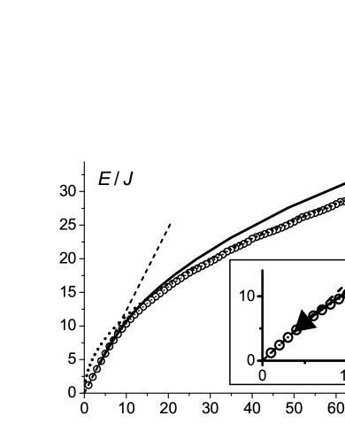
Figure 1: The soliton energy $E$ (in the unity of the exchange integral $J$ ) dependence on the number of magnons $N$ for the case $K=0.7J$. The results of the continual approximation are represented by the solid line, the symbols are results of a numerical analysis of the discrete model, see the next Section. In the inset the detail behavior at small $N$ is present; the arrow’s end points out the end point of the dependence $E(N)$, i.e. minimal value of soliton energy. The symbols beneath the arrow depict delocalized magnon states found by numerical simulation for a finite system. The dash line and doted line represent asymptotic behaviors at $E\to\hbar\omega_{0}N$ and square root asymptotic (19) for small and large $N$, respectively.

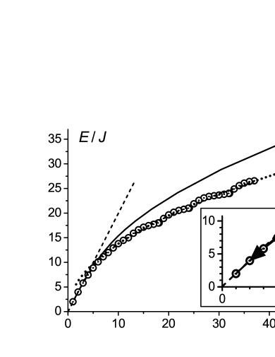
Figure 2: The same as in Fig.1, but for the case $K=0.5J$. Please note essentially smaller values of $N_{\min}$ and $E_{0}$

Thus in the limit cases the dependence of soliton energy on $N$, and also the parameters $J,\;K$ is easily reconstructed. In the intermediate frequency range, which corresponds to numbers of magnons $N$ of the order of few $N_{\min}$ a thorough analysis of (18) is needed. We carried numerical calculations for a set of values of $K/J$ for the region of interest $0<K<J$. The analysis was done as follows: at the given $K/J$ the equation (18) was solved numerically for a set of values of $\omega/\omega_{0}$, which were chosen with different steps. Further having a solution the value of energy $E$ and the number of magnons $N$ were calculated. Then the dependencies $E(N)$ and $\omega(N)$ (the latter is important for analysis of stability of a soliton, which is stable in continual model at $d\omega(N)/dN>0$ only) were constructed.

Let us briefly discuss the main characteristics of solitons found within continual approximation. The analysis confirmed asymptotic dependencies derived above, see Figs. 1,2. In the whole region of parameters of the problem the function $\omega(N)$ monotonously decreases with the $N$ growth, i.e. the stability condition is fulfilled. Thus, in the framework of the continual approximation stable soliton solutions exist within the parameter region $0<K<J$ of Hamiltonian (1). The soliton energies have a lower limit, $E_{0}$, which is smaller then the energy of familiar Belavin-Polyakov solitons.

IV The discreteness effects for longitudinal solitons.

Strictly speaking, the continual approximation is valid only when the characteristic size of a soliton is essentially bigger than the interatomic distance, $|\nabla\theta|\ll 1/a$. This condition may be met for solitons with small amplitude, see (20), and also in the limit case $J-K\ll K$, when the characteristic size $r_{0}$ is larger that the lattice constant $a$, $r_{0}\gg a$. However, in contrast to precessional solitons in Heisenberg magnets with weak anisotropy, in which the characteristic length is tens and hundreds of the lattice constant, in our case the condition $r_{0}\gg a$ is much stricter. Even for enough small $J-K=0.1\cdot J$, the value $r_{0}=1.095\cdot a$ and only slightly exceeds the lattice constant $a$. In the region of the parameters $K\sim J-K\sim J$ and in the especially interesting case $K\ll J$, when the minimal energy of solitons is small, an applicability of this approach is not clear and one can expect essential discreteness effects.

Let us consider the discrete model (7, 8) for a square lattice. Analysis of discrete equations for the variables $\theta_{i}$ and $\phi_{i}$ given for each lattice site demonstrates existence of a solution in the form of $\varphi_{i}=\omega t$ and further it is possible to study only variables $\theta_{i}$.

For analysis of solitons we employ the variation procedure proposed and numerically realized in Ref. Iv+PRB06, . We will seek a conditional minimum of Hamiltonian, in fact, classical energy $W(\theta_{i})$, with respect to variables $\theta_{i}$, under the condition that the number of magnons $N=\sum\nolimits_{i}(1-\cos\theta_{i})$ is fixed. While seeking a minimum one can find the precession frequency $\omega$ from the equation $\partial W/\partial\theta_{i}=\hbar\omega\cdot\sin\theta_{i}$. It is worth noting, the sign of derivative $d\omega/dN$ in a discrete case is not important; a soliton is stable, if the found conditional extreme of energy is minimum. Analysis was done for an approximately circular fragment cut from a square lattice sized $24\times 24$. We limit ourselves to such size as states we are interested in are essentially localized, and the influence of borders on them is negligible, while increase of a sample size require a significant increase of numerical calculation time. As one can expect at small values of $(J-K)/K$ the behavior of the dependencies $E(N)$ and $\omega(N)$ merely follows curves obtained within the continual approximation, therefore we do not present them. As well, for a region of small $N$ our analysis demonstrates that even in the case $r_{0}\leq a$ the results of the continual approximation are quite close to numerical data, see. Fig. 1 and Fig. 2.

It is interesting to note, that even for large $N$, when the characteristic size of inhomogeneity in a solution is of the order of $r_{0}<a$, these results qualitatively describe the dependence $E(N)$ even at moderate values of $K/J$, such as $K/J=0.7$ and $K/J=0.5$, for which $r_{0}=0.54a$ and $r_{0}=0.354a$, respectively. For $K/J=0.7$ numerical data adhere closely continual curves, and a square root dependence with fitted value of domain wall energy $\sigma$ is working rather well. Even for the smaller value $K/J=0.5$ only insignificant sign-alternating deviations from the square root dependence (21), which are almost invisible in Fig. 1 for $K/J=0.7$, are observed on the numerical data on Fig. 2.

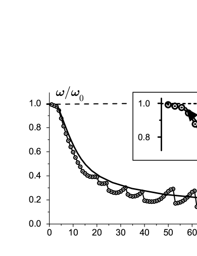
Figure 3: The dependence of the oscillation frequency $\omega$ (in $\omega_{0}$ units) on the number of magnons $N$ for a soliton in the case $K=0.7J$. The results of the continual approximation are shown by the solid line, symbols are a result of the numerical analysis of the discrete model. The horizontal dash line points out theoretical value of magnon gap $\omega_{0}$. In the inset detail behavior at small $N$ is showed, the end of the arrow points out the end point of continual dependence $N=N_{\mathrm{min}}$. Symbols on the left side of the arrow correspond to delocalized magnon states, their insignificant deviations from the value of $\omega_{0}$ are caused by boundary effects, naturally present for a finite system.

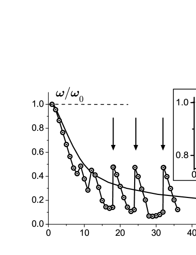
Figure 4: The same as in Fig. 3, for the case $K=0.5J$. The vertical arrows denote special values of $N=18,\;24$ and 32, see the text. Please note that the dependencies correspond each other even at not small $(\omega-\omega_{0})/\omega_{0}\leq 0.25$, that corresponds $N\leq 5$. It is worth to mention that only one nonlocalized state with $N=1$ was revealed.

However, apart from such characteristic of a soliton as $E(N)$, which depends on integral values $E$ and $N$ only, effects of discreteness, nevertheless, are essential. This is apparently demonstrated in the dependence $\omega(N)$, see Fig. 3, 4 and especially it is clearly seen in analysis of the soliton structure, i.e. real distribution $\theta_{i}$ in the lattice, see below. For dependencies $\omega(N)$ when $N$ grows at the beginning, at small $N$ regular deviation of numerical data from the continual curve is observed. This feature can be explained by the fact that $\omega\propto dE/dN$, whereas the energy $E(N)$ in the discrete model is lower than in continuum. However, even for $K/J=0.7$ it was observed noticeable deviations up and down from the smooth dependence typical for continual approximation, see. Fig. 3. For smaller value $K/J=0.5$, this irregular behavior is much more essential, see Fig. 4. This complicated behavior is observed in that region of $N>10\ll N{\mathrm{min}}$ where the effective domain wall approximation and the square root asymptotic (21) should be applicable. Therefore as for precessional solitons in a Heisenberg magnet with strong single-ion anisotropy,Iv+PRB06 it can be naturally associated with characteristics of lattice pinning of a domain wall. Let us discuss the structure of a soliton for $K/J=0.5$, see Fig. 5 and 6.

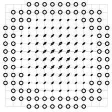
(a)  $N$ =1

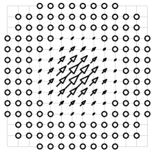
(b)  $N$ =2

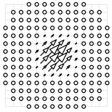
(c)  $N$ =3

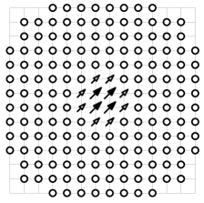
(d)  $N$ =8

Figure 5: Distribution of the discrete variables $\theta_{i}$ and $\phi_{i}$ in a soliton at small $N$ for the system with $K/J=0.5$. Only a small part of fragment chosen for numerical calculation is presented. $\theta$ and $\phi$ for each spin are presented in the form of 3D vector $\boldsymbol{\sigma}=(\sin\theta\cos\phi,\;\sin\theta\sin\phi,\;\cos\theta)$. Values of $5^{0}<\theta_{i}\leq 90^{0}$ are presented by arrows with open heads, while for $90^{0}<\theta_{i}<180^{0}$ by arrows with solid heads, the small values $0\leq\theta_{i}<5^{0}$ are presented by open circles. The transition from non localized state at $N=1$ to localized states at $N>1$ is clearly seen. For $N=3$ the minimal value of $|{\rm{\bf m}}|=|\cos\theta|\approx 0.5$ is observed in the soliton center. For $N=8$, the values of $\theta_{i}$ nearly the soliton center are $158^{0}$ and $15^{0}$, and the tendency of transition to collinear structure is seen.

At small $N$ numerical analysis demonstrates almost radially-symmetric distribution of $\theta_{i}$ with the scale of few lattice constant $a$, that is essentially larger than $r_{0}=0.354a$. It is interesting to note that even such a sensitive parameter as minimal value of $N$ is well reproduced by the continual calculation. According to our continuum calculation, for a magnet with $K/J=0.5$ the value $N_{\min}=1.6$. The discrete analysis provides good localization of a soliton at $N=2,\;3$ and much less localized state at $N=1$, see Fig. 5. With further growth of $N$ up to $N\leq 10$ the distributions of $\theta_{i}$ become much more sharp and tendency of formation of collinear states is observed. For the values of $N\geq 10$ the role of discreteness effects, primarily effects of domain wall pining, increases. This pinning may include either the dependence of the wall energy on its orientation related to lattice vectors or the dependence of the wall energy on its position related to distance to corresponding atomic lines in the lattice.

A set of our numerical results may be explained considering that, like in the case of uniaxial Heisenberg ferromagnet, see Ref. Iv+PRB06, , the most favorable position for a domain wall is to be placed between atomic lines like (0,1) or (1,0), but in contrast to Ref. Iv+PRB06, , the domain wall is quite flexible and its bend from the line (0,1) to (1,0) does not costs too much energy. In principle, it corresponds to conclusions of Gochev,Gochev who has demonstrated that for a 2D discrete classical spin model with anisotropy like (8) pinning effects are present for a domain wall parallel to the axis (0,1) and (1,0) and are absent for a wall parallel to atomic lines like (1,1). On the basis of these assumptions one can describe real distribution of the $\theta_{i}$ amplitude and complicated behavior of $\omega(N)$ in a lattice soliton.

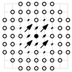
(a)  $N$ =17

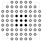
(b)  $N$ =18

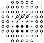
(c)  $N$ =19

Figure 6: The distribution of the discrete variables $\theta_{i}$ for a soliton for $K/J=0.5$ at values of $N$, close to “magic” value $N=18$. Values $0\leq\theta_{i}<5^{0}$ and $175^{0}<\theta_{i}\leq 180^{0}$, corresponding to nearly maximal value of spin along the direction up and down, presented by open and solid circles, respectively, other notations and arrow scale here are the same as in Fig. 5. For collinear structure at $N=18$, as well as for $N=24$ on Fig. 7 below, the mean spin deviation from the nominal value $m=\pm 1$ does not exceed $4\cdot 10^{-5}$. For adjacent values of $N$, deviation from the values $m=\pm 1$ is not small, namely, value $m\approx-0.75$ in the corners of the soliton with $N=17$ and $m\approx 0.6$ in the center of a wall segment at $N=19$.

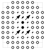
(a)  $N$ =23

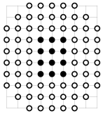
(b)  $N$ =24

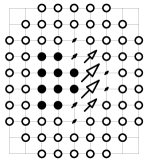
(c)  $N$ =25

Figure 7: The distribution of the discrete variables $\theta_{i}$ in a soliton at $N$, close to “half-magic” value $N=24$. Notations, arrow scale, and the value of $K/J=0.5$ here are the same as in Fig. 6. The value of $m\approx-0.75$ in the corners of the soliton with $N=23$ and $m\approx 0.66$ in the center of a wall segment at $N=25$.

In the case $r_{0}\leq a$ the favorable wall placed between adjacent lines like (0,1) or (1,0) is nearly collinear. Therefore the most favorable values of $N$ are those for which a soliton contains a region where all spins have $m=-1$. The region is separated from the rest of a magnet, where $m=+1$, by segments of such walls. This leads us to such spin configuration, for which this region would be of the form of a rectangular with the size $l_{x}\times l_{y}$, where $l_{x}$ and $l_{y}$ are integers. Apparently, that the most preferable would be square areas with the spin number $l^{2}$ and the magnon number $N=2l^{2}$. Following,Iv+PRB06 let us call these preferable states “magic”. Solitons with $N=N_{\mathrm{magic}}$ have the symmetry axis $\mbox{C}_{4}$ (hereunder we discuss the symmetry axis perpendicular to the lattice plane), and spacious symmetry of a soliton coincides with the lattice symmetry.

Along with magic numbers of magnons $N_{\mathrm{magic}}=2l^{2}$ “half-magic” states with a rectangular of spins in which $l_{x},\;l_{y}$ differ by one and $N=N_{\mathrm{half-magic}}=2l(l+1)$ are also important. Their symmetry is lower then that for solitons with $N=N_{\mathrm{magic}}$ and includes only the axis $\mbox{C}_{2}$. For values like $N=2l(l+2)$ no peculiarities were found, most likely they are always close to magic numbers, $l(l+2)=(l+1)^{2}-1$, and proximity effects to the latter are essential.

Let us explain the character of $\omega(N)$ in a soliton with the value $N$, close to magic number. Configurations with $N<N_{\mathrm{magic}}$ can be obtained by “corner smoothing” of a magic configuration due to wall band inwards “ideal square”, see the example with $N=17$ in Fig. 6. Since this does not require a lot of energy, the frequency in the region $N<N_{\mathrm{magic}}$ is small and faintly depends on $N$, that corresponds well to our numerical calculation. If it is necessary to increase $N$ up to $N>N_{\mathrm{magic}}$, then the situation is different: a domain wall should move into a unfavorable region of the lattice. An increase of $N$ in the region $N>N_{\mathrm{magic}}$ occurs only due to this not profitable wall sector and frequency values in this region are quite large. It is important to note that for a purely collinear state ($\theta=0,\;\pi)$ the change of $\phi$ does not change the system state, and the frequency value has no sense. Therefore at the transition of $N$ through $N=N_{\mathrm{magic}}$ the $\omega(N)$ dependence experiences a jump. For this reason, two values obtained as frequency limit at $N=N_{\mathrm{magic}}+\varepsilon$ and $N=N_{\mathrm{magic}}-\varepsilon$ are sketched in Fig. 4. In real calculation the value $\varepsilon=0.01$ was chosen.

It is worth to discuss an important problem of soliton symmetry. The numerical analysis showed that in this case $N\geq N_{\mathrm{magic}}$ the wall growth occurs only from one soliton side, see for example $N=19$ in Fig. 6. Note the essential lowering of the soliton symmetry for such values of $N$, for which the soliton has no symmetry axis at all. The same regularities take place at the transition through half-magic value, however at $N<N_{\mathrm{half-magic}}$ the soliton symmetry is lower, it contains an element of $\mbox{C}_{2}$ rather than $\mbox{C}_{4}$, see Fig. 7. Then, with increasing of $N$ by values like $2\div 3$ the soliton symmetry is restored. Further when $N$ reaches next chosen number (half-magic after magic or vice versa) this cycle reiterates, see Fig. 4, where the positions of magic numbers $N=18,\;32$ and half-magic number $N=24$ are depicted.

In fact such tendency remains at extremely small values of the ratio $K/J$ up to $K/J=0.1\div 0.3$, when $r_{0}\simeq(0.12\div 0.23)\cdot a\ll a$. Again at $N=1,\;2$ the soliton’s size exceeds $a$, and the soliton can be described within the continuum approximation. Naturally, at small $K/J$ solitons are more localized, for example, at $K/J=0.2$ a purely collinear states appears at smaller $N$ like minimal magic number $N=8$. This quantitative difference leads to qualitatively new feature: at values of $K<K_{\mathrm{(crit)}}\simeq 0.36J$ even the states with $N=1$ are localized. These localized states resembles polarons, which are one-electron states localized due to interaction with non-linear media, see, for example.Nagaev88 These self-localized spin states with $N=1$ can be called spin polarons. It is clear, the detail description of such states with small $N$ should be based on exact quantum analysis, but we believe, our semiclassical consideration gives at least qualitative estimate for energies of such states. For such small $K<K_{\mathrm{(crit)}}\ll J$ the maximal amplitude $\theta(0)$ is not small, the asymptotical solution (20) is not valid more, and the energy of spin polaron state $E^{\mathrm{sp}}\equiv E^{\mathrm{(min)}}$ is smaller then the continual result $8(J-K)$. The value of spin polaron energy equals to $2.57J$ at largest available value of $K=K_{\mathrm{(crit)}}\simeq 0.36J$, and grows till $3.7J$ at $K\ll K_{\mathrm{(crit)}}$.

V Conclusion remarks and result discussion.

We considered spin dynamics in non-Heisenberg magnets with the spin $S=1$ and biquadratic exchange taking into account. For such magnets, there are specific longitudinal magnetic solitons, in the center of which the length of magnetization $\langle S_{z}\rangle$ is smaller than the nominal value $\langle S_{z}\rangle=1$, the values of $\langle S_{x}\rangle$ and $\langle S_{y}\rangle$ are equal to zero, but the oscillations of quadrupolar variables $\langle S_{x}S_{y}+S_{y}S_{x}\rangle$ and $\langle S_{y}^{2}-S_{x}^{2}\rangle$ are presented. The energy of such solitons is smaller then that of standard solitons described within the Landau-Lifshitz equation. In particular this energy is smaller then that for a “transversal” Belavin-Polyakov soliton, for which $|\langle{\rm{\bf S}}\rangle|=1$ and $E_{BP}=4\pi J$. Note that the Belavin-Polyakov soliton, as well as other transversal soliton states, are also presented in the model (1).

Numerical analysis of the discrete lattice model demonstrated applicability of macroscopic approximation in vicinity of $\mathrm{SU}(3)$ point, where $J-K\ll J$. For the rest region of parameters, this approximation is adequate for quantitative (at small $N$) or semi-quantitative, in general case, description of basic characteristics of solitons, for example, the dependence $E(N)$. The analysis of the discrete model has also demonstrated a series of qualitatively new effects, specifically important, when $N$ is large enough and close to some chosen values of the magnon number, magic $N_{\mathrm{magic}}=2l^{2}$ and half-magic $N_{\mathrm{half-magic}}=2l(l+1)$, where $l$ is an integer. For these chosen values a collinear state of solitons is realized, where the magnetization in all points has maximal values $m=\pm 1$.

This result has been obtained within the semiclassical approximation. We were not able to construct such states within exact quantum analysis of the model (1). Let us discuss a role of quantum effects. An important question is whether or not the planar solution survives beyond semiclassical approximation. This problem can be discussed by taking into account the presence of usual ferromagnetic gapless “transversal” magnons within perturbation theory. The existence of an exact semiclassical planar solution means that the equations for transversal variables, linearized over the planar soliton, have zero solution. In terms of magnons, this means that processes of single magnon radiation described by perturbation Hamiltonian $H^{(1)}_{int}=\sum_{k}[\Psi^{(1)}_{\rm{\bf p}}a^{{\dagger}}_{\rm{\bf p}}\exp(i\omega t)+h.c.]$ are absent (hereupon $a_{\rm{\bf p}},\;a_{\rm{\bf p}}^{\dagger}$ are creation and annihilation operators for such magnons with the linear momentum ${\rm{\bf p}}$ and energy $\varepsilon({\rm{\bf p}})\simeq J(ap/\hbar)^{2}$). In principle, there is a possibility for processes with radiation of several magnons, for example, two-magnon process describing by $H^{(2)}_{int}=\sum_{1,2}(\Psi^{(2)}_{1,2}a^{{\dagger}}_{1}a^{{\dagger}}_{2}\exp(i\omega t)+h.c.)$, where $1\equiv{\rm{\bf p}}_{1}$; three-magnon process, etc. Conservation laws of energy, momentum and total $z-$projection of spin, which can be written as $E(N)-E(N-2)=\varepsilon({\rm{\bf p}})+\varepsilon(-{\rm{\bf p}})$, allow this process even at small $E(N)-E(N-2)\simeq 2\hbar\omega\ll J$, as the magnon dispersion law $\varepsilon({\rm{\bf p}})$ has no gap. One can expect the process of decay a soliton to magnons due to such radiations of magnons. As a result, the soliton will be characterized by finite lifetime. Such effects have been discussed early while going beyond the scope of semiclassical approximation for various topological solitons, 2D soliton with non-zero Pontryagin index,IvSheka+PRB07 and 3D soliton characterized by non-zero Hopf index.DzyalIv However, for aforementioned examples these processes are slow and the lifetime of a soliton with large enough $N$ is long, $\tau\sim(\hbar/J)N^{5}$ and $\tau\sim(\hbar/J)N^{5/3}$ in casesIvSheka+PRB07 and,DzyalIv respectively. Therefore one can expect that in our case with complete consideration of quantum effects solitons with large value of $N$ will be enough long-lived excitations. Detailed discussion of this problem goes beyond of the scope of this work.

For solitons in the discrete model one can point out one more interesting quantum effect absent at regular quantization of continual solutions with radial symmetry. For some special numbers of magnons $N$ the lowering of soliton symmetry $\mbox{C}_{4}$ inherent to the square lattice model (1) occurs down to $\mbox{C}_{2}$ or even lower, see above Fig. 6 and 7. The presence of solitons with symmetry lower than lattice symmetry $\mbox{C}_{4}$ means that in the classical case there are several (2 or 4) equivalent states, which differ from each other by orientation in the lattice. In other words the classical state of the soliton is degenerated (two-fold or even four-fold) with regards to the soliton orientation. In the quantum case there is a possibility for quantum tunneling (underbarrier transitions) between these states. For large $N$, the transition probability is low and can be calculated using instanton technique.IvanovFNT05 ; MQT As a result one can expect the splitting of degenerated states, with creation of doublet or multiplet with four levels and lifting of the symmetry of the soliton to $\mbox{C}_{4}$. We plan to return to detailed discussion of these effects in our future work.

It is obvious that observation of effects of “longitudinal” spin dynamics is possible for materials with non-small biquadratic spin interaction. Yet Kittel demonstrated that such interaction appears due to interaction of spin system with lattice deformations.Kittel For common reason, other mechanisms like electric multipole interactions and the Jahn-Teller effect equally resulting in biquadratic exchange (see, e.g., Ref. Levy, ). There are a lot of such materials widely known, among them there are almost isotropic magnets, see review of Nagaev.Nagaev88

In summary it is worth to discuss a possibility of experimental excitation of longitudinal nonlinear spin dynamics in the model (1) considered above. For a standard resonant method two problems come up. First, frequencies of these modes are rather high; second, magnetic field is coupled with dipole variables (magnetization) only and does not influence directly on quadrupolar variables. Both these problems can be solved by usage of ultrashort intensive laser pulse, see, e.g., Refs. Kimel1, ; Kimel2, and for review Ref. exper-rew, . Usual value of a pulse duration $\tau$ can be as short as 100 fs, and frequencies $\omega\geq 1/\tau$, being considerably higher than frequencies of regular spin oscillations can be effectively excited.

The possible role of different variables, dipolar and quadrupolar, can be demonstrated by a simple example. Consider a thick plane – parallel plate of a ferromagnet saturated along its normal ($z$ axis). Let the light pulse propagates along the $z$ axis, with the electric field parallel to the plate surface. The light interaction with dipolar degrees of freedom $m_{i}=\langle S_{i}\rangle$ can be described as following. Due to inverse Faraday effect, a circularly polarized light is equivalent to pulse magnetic field parallel to $z$ axis.Kimel1 ; Kimel2 Linearly polarized light produces two-fold anisotropy in the sample’s plane.PulseGarnets Both scenario are ineffective for a sample, saturated along $z-$axis, and the excitation of usual transversal spin oscillations (magnons) is absent in this geometry.

In contrast, the quadrupolar variables like $\langle S_{i}S_{j}+S_{j}S_{i}\rangle$ with $i,j=x,y$ are coupled directly with linearly polarized light. The influence of such light pulse is equivalent to the direct action of some pulse of effective magnetic field ${\rm{\bf H}}^{Q}(t)$, see Eq. (15), on the variable $\boldsymbol{\sigma}$ of the form $H^{(int)}=-{\rm{\bf H}}^{Q}\boldsymbol{\sigma}$. Being directed perpendicularly to the “ground state magnetization” $\boldsymbol{\sigma}=\mathbf{e}_{z}$, this pulse field effectively excite the oscillations of the $x$ and $y$ components of $\boldsymbol{\sigma}$, that is, the longitudinal spin oscillations considered in this article. The excitation of non-dipolar spin degrees of freedom by use of ultrafast optical pumping was recently observed for magnetic Mott insulator R₂CuO₄.Pisarev+

We are thankful to V. G. Bar’yakhtar, A. K. Kolezhuk and D. D. Sheka for stimulated discussions. The work is partially supported by the grant INTAS-05-1000008-8112 and by the joint grant from Ministry of Education and Science of Ukraine and Ukrainian State Foundation of Fundamental Research F25.2/081.

References

- (1) A. G. Gurevich and G. A. Melkov, Magnetization Oscillations and Waves (CRC Press, New York, 1996).
- (2) V. G. Baryakhtar, B. A. Ivanov, M. V. Chetkin, Sov. Phys. Usp. 28, 563 (1985); V. G. Baryakhtar, M. V. Chetkin, B. A. Ivanov and S. N. Gadetskii, Dynamics of topological magnetic solitons. Experiment and theory, Springer Tract in Modern Physics 139, Springer-Verlag, Berlin, (1994).
- (3) A. M. Kosevich, B. A. Ivanov, and A. S. Kovalev, Phys. Rep. 194, 117 (1990).
- (4) H.-J. Mikeska and M. Steiner, Adv. Phys. 40, 191 (1991).
- (5) V. G. Bar’yakhtar and B. A. Ivanov, Solitons and Thermodynamics of Low–Dimensional Magnets, in: Soviet Scientific Reviews, Section A. Physics, I. M. Khalatnikov (ed.), 16 (1992)
- (6) B. A. Ivanov, Low Temp. Phys. 31, 635 (2005).
- (7) A. I. Akhiezer, V. G. Bar’yakhtar, and S. V. Peletminskii, Spin Waves, North-Holland, Amsterdam (1968).
- (8) H. H. Chen and P. M. Levy, Phys. Rev. Lett. 27, 1383 (1971); Phys. Rev. B74, 267 (1973).
- (9) V. M. Matveev, Sov. Phys. JETP 38 813 (1974); Sov. Phys. Solid State 16, 1067 (1974).
- (10) É. L. Nagaev, Sov. Phys. Usp. 25, 31 (1982); É. L. Nagaev, Magnets with Nonsimple Exchange Interactions [in Russian], Nauka, Moscow (1988).
- (11) V. M. Loktev and V. S. Ostrovskiĭ, Low Temp. Phys. 20, 775 (1994).
- (12) B. A. Ivanov and A. K. Kolezhuk, Phys. Rev. B68, 052401 (2003).
- (13) K. Buchta, G. Fáth, Ö. Legeza, and J. Sólyom, Phys. Rev. B 72, 054433 (2005).
- (14) Y. Xian, J. Phys.: Condens. Matter 5, 7489 (1993)
- (15) A. M. Perelomov, Sov. Phys. Usp. 20, 703 (1977); A. Perelomov, Generalized Coherent States and Their Applications Springer-Verlag, Berlin, (1986).
- (16) E. Fradkin, Field theories of condensed matter systems, in Frontiers in Physics, 82, Addison–Wesley (1991).
- (17) E. Beaurepaire, J.-C. Merle, A. Daunois, and J.-Y. Bigot, Phys. Rev. Lett. 76, 4250 (1996).
- (18) A. Scholl, L. Baumgarten, R. Jacquemin, and W. Eberhardt, Phys. Rev. Lett. 79, 5146 (1997).
- (19) J. Hohlfeld, E. Matthias, R. Knorren, and K. H. Bennemann, Phys. Rev. Lett. 78, 4861 (1997).
- (20) F. Hansteen, A. V. Kimel, A. Kirilyuk, and Th. Rasing, Phys. Rev. Lett. 95, 047402 (2005).
- (21) C. D. Stanciu, F. Hansteen, A. V. Kimel, A. Kirilyuk, A. Tsukamoto, A. Itoh, and Th. Rasing, Phys. Rev. Lett. 99, 047601 (2007)
- (22) A. V. Kimel, A. Kirilyuk, F. Hansteen, R. V. Pisarev, and Th. Rasing, J. Phys.: Condens. Matter 19, 043201 (2007).
- (23) Zhou Fei, Quantum Spin Nematic States in Bose-Einstein Condensates, Electronic preprint ArXiv:cond-mat/0108473 (2002).
- (24) B. A. Ivanov and R. S. Khymyn, JETP 104, 307 (2007)
- (25) B. A. Ivanov, JETP Lett. 84, 84 (2006).
- (26) N. A. Mikushina, A. S. Moskvin, Phys. Letters A 302, 8 (2002).
- (27) N. Papanicolaou, Nucl. Phys. B 305, 367 (1988).
- (28) G. B. Whitham, Linear and nonlinear waves, John A Wiley-interscience publication, NY (1974)
- (29) L. D. Landau and E. M. Lifshitz, Electrodynamics of Continuous Media, 1st ed., Pergamon Press, Oxford (1960).
- (30) B. A. Ivanov, C. E. Zaspel, and I. A. Yastremsky, Phys. Rev. B 63, 134413 (2001)
- (31) I. G. Gochev, Sov. Phys.-JETP 58, 115 (1983).
- (32) B. A. Ivanov, A. Yu. Merkulov, V. A. Stephanovich, and C. E. Zaspel, Phys. Rev. B 74, 224422 (2006).
- (33) B. A. Ivanov, D. D. Sheka, V. V. Krivonos, and F. G. Mertens, Phys. Rev. B 75, 132401 (2007)
- (34) I. E. Dzyaloshinskii and B. A. Ivanov, JETP Lett. 29, 592 (1979).
- (35) E. M. Chudnovsky and J. Tejada, Macroscopic Quantum Tunneling of the Magnetic Moment (Cambridge University Press, Cambridge, 1998).
- (36) C. Kittel, Phys. Rev. 120, 335 (1964)
- (37) P. M. Levy, in Magnetism in Metals and Metallic Compounds, edited by J. T. Lopuszanski, A. Pekalski, and J. Przystawa, Plenum Publishing Corp., New York, (1976).
- (38) E. A. Turov, A. V. Kolchanov, V. V. Menshenin, I. F. Mirsaev, V. V. Nikolaev, Symmetry and physical properties of antiferromagnets (Fizmatlit, Moscow, 2001) (in Russian).
- (39) A. K. Zvezdin and V. A. Kotov, Modern Magneto-Optics and Magneto-Optical Materials (IoP Publishing, Bristol, 1997).
- (40) A. V. Kimel, A. Kirilyuk, A. Tsvetkov, R. V. Pisarev, and Th. Rasing, Nature 429, 850 (2004).
- (41) A. V. Kimel, A. Kirilyuk, P. A. Usachev, R. V. Pisarev, A. M. Balbashov, and Th. Rasing, Nature 435, 655 (2005).
- (42) V. V. Pavlov, R. V. Pisarev, V. N. Gridnev, E. A. Zhukov, D. R. Yakovlev and M. Bayer, Phys. Rev. Lett. 98, 047403 (2007).