Thermodynamics and Dynamics of a Monoatomic Glass-Former. Constant Pressure and Constant Volume Behavior

Abstract

We report constant-volume and constant-pressure simulations of the thermodynamic and dynamic properties of the low-temperature liquid and crystalline phases of the modified Stillinger-Weber (mSW) model. We have found an approximately linear increase of the effective Gaussian width of the distribution of inherent structures. This effect comes from non-Gaussianity of the landscape and is consistent with the predictions of the Gaussian excitations model representing the thermodynamics of the configurational manifold as an ensemble of excitations, each carrying an excitation entropy. The mSW model provides us with both the configurational and excess entropies, with the difference mostly attributed to vibrational anharmonicity. We therefore can address the distinction between the excess thermodynamic quantities often used in the Adam-Gibbs (AG) equation. We find a new break in the slope of the constant pressure AG plot when the excess entropy is used in the AG equation. The simulation diffusivity data are equally well fitted by applying a new equation, derived within the Gaussian excitations model, that emphasizes enthalpy over entropy as the thermodynamic control variable for transport in viscous liquids.

I Introduction

Both thermodynamic and dynamic properties of structural glass-formers are unusual and not fully understood.Ngai (2000); Angell (1995) It has long been suggested that puzzles of the dynamics of supercooled liquids can be unraveled from the properties of their energy landscapes.Goldstein (1969) Attempts to build a description of dynamics based on the liquid thermodynamics go back to the Adam-Gibbs (AG) theoryAdam and Gibbs (1965) which emphasizes configurational entropy as the origin of non-Arrhenius dynamics. Even though the entropic paradigm seems to be currently most successful in describing relaxation,Xia and Wolynes (2000, 2001); Lubchenko and Wolynes (2004) other approaches have emphasized the energetic aspects of the problem in terms of the activated kinetics over enthalpic barriers increasing in height with lowering temperature.Goldstein (1969); Bässler (1987); Arhipov and Bässler (1994); Dyre (1995); Matyushov and Angell (2005) Some very recent dataDalle-Ferrier et al. (2007) seem to disfavour the existence of diverging lengthscale assumed in “cooperative region” modelsAdam and Gibbs (1965); Xia and Wolynes (2000) supporting instead the picture of activation-based dynamics in glass-forming materials.

Configurational entropy is a property not directly accessible from laboratory experiment, but is increasingly available from computer simulations of model systems.Sastry (2001); Saika-Voivod et al. (2001); Mossa et al. (2002); Giovambattista et al. (2003); Saika-Voivod et al. (2004); Gebremichael et al. (2005) Excess entropy, $s^{\text{ex}}_{P,V}(T)$, i.e. the liquid entropy over that of the thermodynamically stable crystal, has been successfully usedAngell (1991); Richert and Angell (1998) instead of configurational entropy $s^{c}_{P,V}(T)$ in the AG relation

$$\ln(\tau_{P,V}(T)/\tau_{0})=\frac{\Delta}{Ts^{c}_{P,V}(T)},$$ (1)

where $\tau_{P,V}(T)$ is the time of structural relaxation and $\tau_{0}$ is the time characteristic of quasi-lattice vibrations. The subscripts $P,V$ in the entropy and relaxation time specify the conditions, constant-pressure ($P$) or constant-volume ($V$), at which the entropy and the relaxation time are measured. Historically, the definition of the configurational entropy used by Adam and GibbsAdam and Gibbs (1965) was that of the full configurational entropy including the entropy of basin vibrations. However, since they explicitly demanded the vibrational entropy to cancel between the liquid and the crystal, their configurational entropy is in fact the entropy of inherent structure introduced by Stillinger and Weber (see below).Stillinger and Weber (1982) We will therefore refer to the configurational entropy in this latter definition.

The full configurational entropy and Stillinger’s entropy of inherent structures are in fact not equivalent. Most studies, both laboratoryGoldstein (1976); Phillips et al. (1989); Corezzi et al. (2004) and computational,Sastry (2001); Mossa et al. (2002); Giovambattista et al. (2003) have shown that the excess entropy has a significant contribution from the vibrational manifold related to the excess density of vibrational states in liquid, $g_{P,V}^{\text{liq}}(\omega)$, compared to the crystal, $g_{P,V}^{\text{cryst}}(\omega)$. The excess vibrational entropy from harmonic motions is a sum over the vibrational spectrum:

$$\Delta s^{h}_{P,V}=\sum_{\omega}\left[g^{\text{liq}}_{P,V}(\omega)-g^{\text{cryst}}_{P,V}(\omega)\right]\ln(\omega).$$ (2)

So long as the structure does not change, the excess density of states is independent of temperature for purely harmonic vibrations resulting in a temperature-independent excess harmonic entropy $\Delta s_{P,V}^{h}$ and zero contribution to the excess heat capacity. The anharmonicity of atomic and molecular vibrations leads to two effects: (i) sample expansion at constant-pressure heating and (ii) deviations of the vibrational excess entropy $\Delta s^{\text{vib}}_{P,V}$ from the harmonic formula in Eq. (2). The first effect makes the density of quasi-harmonic vibrations vary with temperature and the second effect requires extracting the thermodynamics of vibrations without relying on the harmonic approximation [Eq. (2)].

For most systems studied to date, the density of quasi-harmonic vibrations is known to depend weakly on temperature except for the low-frequency feature known as the Boson peak. The excess vibrational density of states from this region in liquid selenium was shown to produce ca. 30% of both the excess entropy and heat capacity.Phillips et al. (1989) These results, and the puzzling ability of both the configurational (simulations) and excess (laboratory) entropies to fit the relaxation data according to Eq. (1), have lead to the suggestion that configurational and excess entropies of glass formers might be proportional to each other.Martinez and Angell (2001); Angell and Borick (2002) There are simulationStarr et al. (2003) and laboratoryCorezzi et al. (2004) data in support of this proposal, although the question is still not fully settled.Johari (2007)

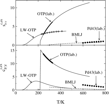
Figure 1: Excess (for laboratory data) and configurational (for computer simulations) entropy (a) and heat capacity (b) of some glass-forming liquids: glass-forming alloy Pd₄₃Cu₂₇Ni₁₀P₂₀ (Pd43),Lu et al. (2002) o-terphenylMoynihan and Angell (2000) (OTP) and their computer models, binary mixture Lennard-Jones (BMLJ)Kob and Andersen (1994) and Lewis and Wahnström o-terphenyl (LW-OTP).Mossa et al. (2002) The closed points and thick lines are laboratory data, the open points and dashed lines are computer simulations, and the thin lines are fits to the 1G excitations model (from Ref. Matyushov and Angell, 2007).

The resolution of the problem of partitioning the excess entropy and heat capacity between vibrational and configurational manifolds is not straightforward. Recent experimental data have argued in favor of both a negligible contribution of vibrations to the excess heat capacity Johari (2007) and a significant contribution amounting from 30% (Refs. Phillips et al., 1989 and Corezzi et al., 2004) to 50–60% (Refs. Angell et al., 2003 and Wang and Richert, 2007). Computer models do not tend to help much in resolving this issue due to a general disconnect between simulated and experimental results. The situation is illustrated in Fig. 1 where excess (laboratory experiment) and configurational (computer simulations) thermodynamic quantities are compared for two substances, $o$-terphenyl and the glass-forming alloy Pd₄₃Cu₂₇Ni₁₀P₂₀, for which both force-field modelsLewis and Wahnström (1994); Kob and Andersen (1994) and experimental resultsMoynihan and Angell (2000); Lu et al. (2002) are available. For $o$-terphenyl, there is a major difference in both the magnitude and temperature dependence of the entropy and heat capacity, though this is not unexpected given that a flexible 14-carbon molecule is being modeled with a rigid three-bead particle (making it much less entropic). The difference is not removed by comparing the experiments with the limited simulation data available for constant pressure.Angell et al. (2003) For Pd₄₃Cu₂₇Ni₁₀P₂₀ glass-former, as modeled by Kob and co-workers binary mixture,Kob and Andersen (1994) the agreement is better and a noticeable difference exists only for the heat capacities, however the need for many components in the experimental analog is a disadvantage.

Clearly, to resolve the question of vibrational contributions to the excess heat capacity, the field is in need of better model systems. A minimum need is for a system in which both excess and configurational data are available, something so far lacking in computer models (except for waterStarr et al. (2003) which is famously anomalous and unrepresentative of the glass problem we are addressing). The recent exploration of the Stillinger-Weber type model by Molinero et al.Molinero et al. (2006) offers an opportunity to fill this gap since the crystal state is available and, for chosen parametrizations, the liquid can be supercooled without limit. Our simulations here take advantage of this opportunity.

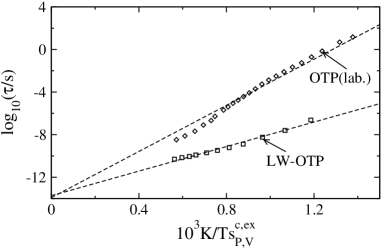
Figure 2: Adam-Gibbs plot of the experimental dielectric relaxation data of $o$-terphenyl (OTP)Richert and Angell (1998) and simulated self-diffusivityMossa et al. (2002) of Lewis and Wahnström o-terphenyl (LW-OTP, NVT simulations). Excess entropy (at constant pressure) was used for experimental points and configurational entropy (at constant volume) for simulated data. The dashed line is a linear fit through the data with the intercept at $\tau_{0}=10^{-14}$ s. The simulation data are shifted vertically to cross the vertical axis at about the same relaxation time. The Adam-Gibbs relation does not linearize the dielectric data in the whole range of temperatures displayed,Richert and Angell (1998) and the plot only serves to illustrate the difference in the range of Adam-Gibbs parameter $(Ts^{c,\text{ex}}_{P,V}(T))^{-1}$ and relaxation times explored by simulations ($V=Const$) and experiment ($P=Const$).

Many recent simulations have offered access to both configurational thermodynamics and dynamics reporting the success of the AG relationScala et al. (2000); Sastry (2001); Mossa et al. (2002); Gebremichael et al. (2005) [Eq. (1)]. As mentioned above, the low-temperature part of experimental relaxation data can be fitted by the same relation where $s^{\text{ex}}_{P,V}(T)$ is used instead of $s^{c}_{P,V}(T)$.Richert and Angell (1998) While this creates a puzzling contradiction, one needs to keep in mind the difference in the scales of the two sets of data, which is illustrated in Fig. 2 comparing the laboratory dielectric dataRichert and Angell (1998) for OTP with the results of simulationsMossa et al. (2002) for the Lewis and Wahnström (LW) model of OTP.Lewis and Wahnström (1994) The difference in slopes of simulations and laboratory data may originate from the use of different ensembles, constant volume and constant pressure, respectively, and of different entropies, configurational and excess. The AG relation in fact linearizes the laboratory data only at low temperatures, below the crossover temperature $T_{x}$ associated with either the mode-coupling critical temperature or the temperature $T_{b}$ of the Stickel analysis.Richert and Angell (1998) The experimental data can be linearized in the AG plot with different slopes below and above $T_{x}$, as we also describe below for the modified Stillinger-Weber (mSW) model, when the excess entropy is used in the AG plot.

Both the range of temperatures and the property studied can affect the conclusions regarding the validity of the AG relation from the simulation data. This is illustrated for SPC/E water in Fig. 3. The dielectric relaxation times collected from Molecular Dynamics (MD) simulations in a broad range of temperaturesGhorai and Matyushov (2006) show a break in the slope of the AG plot (configurational entropy is taken from Ref. Starr et al., 2003). The change in slope is much less pronounced for the one-particle rotational and translational relaxation times (triangles and diamonds in Fig. 3) than for the many-particle Debye relaxation time (circles in Fig. 3). Diffusivity was the only dynamic property considered in the original report of success of the AG relation for SPC/E water,Scala et al. (2000) which indeed shows almost linear AG plot. Notice that the change of the slope seen in the simulation data in Fig. 3 is uniformly observed in laboratory dielectric measurements of a number of glass-formers.Richert and Angell (1998) However, a downward break in the slope, in contrast to the upward-curved dependence seen for SPC/E water in Fig. 3, is typically obtained for molecular glass-formers, as is also the case with the AG plot of the mSW model discussed below. In case of water, this discussion should be supplemented by the question of the relevance of the AG plot to the approach to a thermodynamic (near-critical) singularity.Xu et al. (2005)

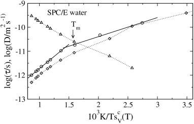
Figure 3: Diffusivity (triangles), relaxation time of one-particle rotational diffusion (diamonds), and Debye relaxation time (circles) of SPC/E waterGhorai and Matyushov (2006) vs $1/(Ts^{c}_{V}(T))$ with configurational entropies taken from Ref. Starr et al., 2003. The dotted lines connect the points, the solid lines are linear regressions through high- and low-temperature portions of the dielectric relaxation data. $T_{m}=273$ K indicates the melting temperature of laboratory water at ambient conditions.

Two of us have recently suggested to describe the thermodynamics and dynamics of glass-forming liquids close to $T_{g}$ in terms of configurational excitations with a Gaussian distribution of excitation energies (Gaussian excitations model).Matyushov and Angell (2005, 2007) Entropy, calculated from microcanonical ensemble, was the starting point for developing the theory. Each excitation was assumed to carry the excess entropy $s_{0}$ which was subdivided into configurational and vibrational parts, $s_{0}=s_{0}^{\text{vib}}+s_{0}^{c}$. These excitation entropies and the number of configurations of an ideal gas of excitations provide the excess and configurational components of the entropy. The excess entropy is connected to the configurational entropy by the relation

$$s_{P,V}^{\text{ex}}(T)=s_{P,V}^{c}[x(T),T]+x(T)s_{0}^{\text{vib}}.$$ (3)

The effect of the vibrational excitation entropy $s_{0}^{\text{vib}}$ is not limited to the last term in Eq. (3) since the excited-state population $x(T)$ is determined by the total excitation entropy $s_{0}$ and the excitation energy $\epsilon_{0}$:

$$x(T)=\left(1+\exp\right[s_{0}-\beta(\epsilon_{0}-2x(T)\lambda)\left]\right)^{-1},$$ (4)

where $\beta$ is the inverse temperature. The energies of excitations are assumed to belong to a Gaussian distribution with the width $2\lambda T$ and the Gaussian width parameter $\lambda$. This energy lowers the energy of excitations in Eq. (4) to the extent determined by the excited state population and $\lambda$, $\epsilon(T)=\epsilon_{0}-2x(T)\lambda$, thus producing a self-consistent equation for $x(T)$.

The excess vibrational entropy originating in the excess density of states of a liquid relative to its crystal provides an extra driving force, in addition to the larger number of basins, for the system to reach the top of its energy landscape.Goldstein (1976) This extra entropic driving force will lead to an increased fragility of the liquid if the excited state population change occurs in the temperature range of interest (near $T_{g}$). In such a case, changes in the excess density of vibrational states will be observable directly through neutron scattering study of glasses of different fictive temperatures, as has been reported for some cases. However, there are strong theoretical suggestionsMatyushov and Angell (2005, 2007) that in the case of very fragile liquids the excited state is highly populated above $T_{g}$ (due, in principle, to an earlier phase transition below $T_{g}$Matyushov and Angell (2005, 2007)) in which case the excess entropy due to vibrations (which can be quite significantGoldstein (1976); Angell and Borick (2002)) will change little with temperature. There will be a vibrational entropy difference from the crystal due to different vibrational density of states [Eq. (2)], but there will be no temperature dependence to this excess. The higher heat capacity of the fragile liquid must then have some other source. One such source could lie in the $T$-dependence of the Gaussian width of the excitation profile, which will be addressed below.

This conclusion is, of course, limited by the assumption that $s_{0}^{\text{vib}}$ is temperature-independent. This assumption in fact implies the neglect of vibration anharmonicity making eigenvalues of the landscape basins depend on temperature, also including the effect of thermal expansion. If this assumption is violated,Angell et al. (2003) a vibrational contribution appears in the excess heat capacity. We found, however, that the assumption of $s_{0}^{\text{vib}}=Const$ describes laboratory fragile liquids well and also found that common model fluids used in simulations classify as intermediate/strong in terms of their fragility.Matyushov and Angell (2005, 2007)

For intermediate and strong liquids, the temperature change in the configurational entropy is driven by the changing population of the configurationally excited state, as was the case in the original two-state Angell-Wong model.Angell and Wong (1970) In this case, the temperature dependence of $x(T)$ in Eq. (3) contributes to the heat capacity, and there is a non-zero vibrational component in the excess heat capacity.Angell and Borick (2002) A nonzero $s_{0}^{\text{vib}}$ is therefore sufficient to produce a vibrational excess heat capacity for intermediate/strong liquids, while this property should be temperature-dependent for a vibrational excess heat capacity to exist for fragile liquid.

The distinction between the thermodynamics of fragile and strong glass-formers is attributed in the Gaussian excitations model to two parameters: critical excitation entropy and critical temperature. In order for the fragile behavior to be realized, the excitation entropy should be higher than the critical value $s_{0c}\simeq 2$ and the temperature should be lower than $T_{c}=\lambda/2$. The binary mixture Lennard-Jones (BMLJ) liquids, which we have analyzed previously,Matyushov and Angell (2007) and the mSW liquid analyzed here all have excitation entropies falling below the critical value and thus classify as strong/intermediate liquids. The excess heat capacity of the mSW liquid has, therefore, a vibrational component $\simeq 15$ % as discussed below.

The dynamic part of the excitation modelMatyushov and Angell (2007) has offered an expression for the relaxation time alternative to the AG formula in terms of the configurational heat capacity instead of the configurational entropy:

$$\ln(\tau/\tau_{0})=\frac{DT^{\prime}}{T-T^{\prime}c_{P}^{c}(T)},$$ (5)

where $D$ and $T^{\prime}$ are model parameters varied in fitting the experiment. This relation gives the fits of relaxation times from laboratory and computer experiments comparable to those based on the AG relation. However, it carries a problem similar to the one encountered in applications of the AG equation. The experimental data can be fitted by using the excess heat capacity, $c_{P}^{\text{ex}}$, while simulation data can be accounted for with the configurational part $c_{P}^{c}$. Here we offer some insights into this problem from the data collected for the mSW model.Molinero et al. (2006)

Some predictions of the excitations model deviate from popular models of landscape thermodynamics. The concept of potential energy landscape, proposed by Goldstein,Goldstein (1969) was formalized by Stillinger and WeberStillinger and Weber (1982) in terms of the thermodynamics of inherent structures reducing the many-body problem of describing liquids to a single “reaction coordinate” $\phi$ defined as the depth of the potential energy minimum (per molecule, $\phi=\Phi/N$, $N$ is the number of molecules). The probability to find a minimum of depth $\phi$ is determined by the number of minima of given depth $\Omega(\phi)$ and two free energies, the total thermodynamic free energy $f(T)$ and the free energy $f^{b}(\phi,T)$ of the system exploring the phase space within the basin surrounding the minimum of depth $\phi$:

$$N^{-1}\ln\left[P(\phi,T)\right]=-\beta\phi+\omega(\phi)+\beta\left[f(T)-f^{b}(\phi,T)\right].$$ (6)

Here, $\omega(\phi)=N^{-1}\ln[\Omega(\phi)]$ is the enumeration function. The subscript specifying ensemble (constant volume or constant pressure) is omitted in Eq. (6) for brevity. In case of constant-volume conditions, $f(T)$ is the common notation for the free (Helmholtz) energy per particle. At constant pressure, $f(T)$ should be understood as the Gibbs energy and $\phi$ is the potential enthalpy minimum.Stillinger (1998) We will drop the ensemble specification in the landscape variables below reserving it to the equilibrium properties, e.g. $c_{P,V}^{c}(T)$, where this distinction is critical.

The formalism of inherent structures is particularly convenient when $f^{b}(\phi,T)$ is independent of $\phi$. Otherwise, Eq. (6) is formally a definition of the basin free energy. It was found that at high temperatures accessible to simulations the harmonic part of $f^{b}(\phi,T)$ is a weak linear function of $\phi$.Starr et al. (2001); Mossa et al. (2002) The main focus of the formalism is, however, on the enumeration function. It is a decreasing function with lowering $\phi$ allowing the liquid to explore higher energy states with increasing temperature (entropy drive). It was suggested that Derrida’s Gaussian model,Derrida (1981) originally derived for glasses with quenched disorder,Fischer and Hertz (1999) can be extended to quasi-equilibrated supercooled liquids with the result that $\omega(\phi)$ is an inverted parabola with a temperature-independent curvature:

$$\omega(\phi)=\omega_{0}-\frac{(\phi-\phi_{0})^{2}}{2\sigma^{2}}.$$ (7)

Even though combinatorial arguments suggest that the parabolic approximation should fail at low temperatures,Stillinger (1988); Shell and Debenedetti (2004) the high-temperature portion of $\omega(\phi)$ is supported by simulations of Lennard-Jones (LJ) mixtures.Büchner and Heuer (1999); Sastry (2001) A more stringent test of the Gaussian model comes from considering the temperature dependence of the average basin depth $\bar{\phi}_{V}(T)$ which, in the Gaussian model, is predicted to scale linearly with $1/T$, producing a $1/T^{2}$ scaling for the configurational heat capacity. Most available simulations report deviations from this scaling.Sastry (2000); Sciortino (2005); Moreno et al. (2006); Matyushov (2007) It is currently not fully established whether the origin of this deviations should be traced back solely to anharmonicity effectsSastry (2000) or to the actual failure of the Gaussian approximation although two recent simulations exploring the low-temperature part of the landscape point to the latter explanation.Moreno et al. (2006); Matyushov (2007) In the excitations model, the temperature dependence of the average basin energy is qualitatively different for fragile and intermediate liquids. In the former case, the basin energy is essentially flat for fragile liquids terminating through a discontinuity at the phase transition below $T_{g}$. For intermediate liquids, $\bar{\phi}_{V}(T)$ starts to dip as $1/T$ from a high-temperature plateau (as was found for the BMLJ liquidsSastry (2001)) and then inflects into an exponential temperature dependence recently observed in simulations of model network glass-formers.Moreno et al. (2006) Note that the excitations model is the only analytical model we are aware of which incorporates both types of temperature scaling in one formalism.

The Gaussian excitations model leads to a non-Gaussian $P(\phi)$ and thus a non-parabolic $\omega(\phi)$.Matyushov and Angell (2005) When the non-Gaussian distribution $P(\phi)$ is fitted to a Gaussian function, the result is an approximately linear scaling of the squared width with temperature $\sigma_{P,V}^{2}(T)\propto T$. This results makes $P(\phi)$ in Eq. (6) a Boltzmann distribution, which seems to be more relevant for a (quasi)equilibrated supercooled liquid than the non-Boltzmann distribution of the Gaussian landscape more relevant for systems with quenched disorder. In addition, the excitations model gives hyperbolic temperature scaling for the heat capacity $c_{P,V}^{c}\propto 1/T$. This scaling is often observed in the laboratory for $c_{P}^{\text{ex}}(T)$, but here we again face the same problem as above concerning the connection between excess and configurational heat capacity.

An approximately linear scaling of the width of $P(\phi)$ with temperature in the excitations model is the result of the assumed mean-field, infinite-range attraction between the excitations, which is equivalent to assuming a Gaussian manifold of real-space excitation energies with the variance $2\lambda T$. A finite range of interactions between the excitations will produce a more complex temperature dependence. For instance, a recent exactly solvable landscape model of the fluid of dipolar hard spheresMatyushov (2007) gave a fairly complex temperature scaling of the distribution variance $\sigma_{V}^{2}(T)\propto(1+\beta b)^{-3}$ ($b$ is an interaction parameter). Notice in this regard that a fluid with dipolar interactions is an archetypal system in which the mean-field approximation is not applicable. The reason is two-fold: (i) the average of the potential is zero and fluctuations is the first non-vanishing contribution to the thermodynamicsOsipov et al. (1997) (cf. to LJ forces described reasonably by the mean-field van der Waals model) and (ii) the interaction potential is strongly anisotropic. How the model should be extended to a finite range of correlations between the excitations is not clear now, but the distribution width is expected to transform to a temperature-independent value for isotropic short-range LJ forces, in compliance with the Gaussian model [Eq. (7)]. Any non-Gaussian landscape will generate a temperature-dependent width when distribution of inherent energies is fitted by a Gaussian.

Table 1: Thermodynamic parameters (energies in kelvin and entropies in $k_{\text{B}}$ units) of mSW and BMLJ models.

Model	$\epsilon$	$T_{m}$	$T_{K}^{c}$	$T_{K}^{\text{ex}}$	$T_{0}$	$-\phi_{\text{IG}}$	$-\phi_{\text{DC}}$	$\omega_{0}$	$s_{0}^{\text{ex}}$	$s_{0}^{c}$
mSW ($\lambda=19$)	25150	806	434	392	420	49482	50300	1.20	2.4	1.0
BMLJ ($\rho=1.2$)	120		35					0.93		0.32

In this paper, we use the results of simulations of the mSW potential to address some of the challenges listed above. We present the results for the landscape thermodynamics for two values of the tetrahedrality parameter $\lambda$ of the mSW potential (see below) and will compare the results of the analysis to some other models of glass-formers on one hand and to laboratory data for metallic glass-formers on the other. Some thermodynamic parameters relevant to our discussion are listed in Table 1. All energies throughout below are in kelvin and entropies and heat capacities are in units of $k_{\text{B}}$. Also, we use low-case letters for thermodynamic potentials and energies per liquid particle, e. g. $s^{c}_{P,V}(T)$ refers to the configurational entropy per particle.

II Landscape Thermodynamics

The properties of the energy landscape for a given interaction potential can be studied by either a direct calculation of the enumeration function $\omega(\phi)$ or by looking at the ensemble averages.Stillinger (1998) In the first route, $\omega(\phi)$ is calculated by patching together the distribution functions at different temperatures once the total and basin free energies entering Eq. (6) are known.Sastry (2000); Sciortino (2005); Matyushov (2007) The width of each individual distribution scales as $1/\sqrt{N}$ with the number of particles $N$, and most simulation data allow a Gaussian fit

$$P(\phi)\propto e^{-N\left(\phi-\bar{\phi}_{P,V}(T)\right)^{2}/2\Gamma_{P,V}(T)^{2}}.$$ (8)

Here, $\Gamma_{P,V}(T)$ is an empirical Gaussian width and the stationary point $\bar{\phi}_{P,V}(T)$ is the solution of the equation

$$\beta\left(1+\partial f^{b}(\phi,T)/\partial\phi\right)=\partial\omega(\phi)/\partial\phi.$$ (9)

When $f^{b}(\phi,T)=f^{b}(T)$ is independent of $\phi$ (harmonic approximation) and the enumeration function is given by the inverted parabola [Eq. (7)], one gets the hyperbolic temperature scaling

$$\bar{\phi}_{P,V}(T)=\phi_{0}-\frac{\sigma^{2}}{T}$$ (10)

characteristic of the Gaussian landscape.

The configurational entropy is determined by the enumeration function taken at the average basin depth

$$s^{c}_{P,V}(T)=\omega(\bar{\phi}_{P,V}(T)).$$ (11)

The configurational entropy is then a part of the thermodynamic free energy $f(T)$

$$f(T)=\bar{\phi}_{P,V}(T)-Ts^{c}_{P,V}(T)+f^{b}[\bar{\phi}_{P,V}(T),T].$$ (12)

Once both $\bar{\phi}_{P,V}(T)$ and $s^{c}_{P,V}(T)$ are known, the enumeration function $\omega(\phi)$ can be calculated using Eq. (11).Stillinger (1998)

III Simulation details

We use a model of network liquids which was originally introduced by Stillinger and Weber (SW)Stillinger and Weber (1985) for silicon. In the SW model, a three-body term is added to the pairwise potential $v_{2}(r)$ to introduce penalty for deviating from tetrahedrality

$$v(r_{12},r_{23},r_{31})=v_{2}(r_{12})+\lambda v_{3}(r_{12},r_{23},r_{31})$$ (13)

where

$$v_{2}(r)=\left\{\begin{array}[]{lll}&&A(B/r^{4}-1)\exp(r-a)^{-1}),r<a\\ &&0,r\geq a\end{array}\right.$$ (14)

with $A=7.049555277$, $B=0.602245584$, and $a=1.8$. The three body potential has form

$$v_{3}(r_{12},r_{13},\theta_{213})=\exp[\gamma(r_{12}-a)^{-1}+\gamma(r_{13}-a)^{-1}]\times(3\cos\theta_{213}+1)^{2}/9$$ (15)

with $\gamma=1.2$. The potentials are given in reduced units $\sigma=0.20951$ nm and $\epsilon=50$ kcal/mol (see also Table 1).

The original SW model with $\lambda=21$ describes silicon, but was modified recently by Molinero et al.Molinero et al. (2006) by decreasing the tetrahedrality parameter $\lambda$ (in contrast to its increase attempted earlier by Middleton and WalesMiddleton and Wales (2001)) to obtain monoatomic glass-formers. They showed that the system crystallizes into diamond cubic (DC) lattice for $\lambda>20.25$ and into body-centered cubic (BCC) lattice for $\lambda<17.5$. For intermediate values of $\lambda$ the fluid fails to crystallize on the time-scale of computer simulation, producing glass-formers.

Since each fluid, characterized by a given value of $\lambda$, has an equilibrium crystalline phase, this property can be used to obtain both the excess and configurational thermodynamics for the same system. Two fluids have been used in simulations: the original SW model ($\lambda=21$) and mSW model ($\lambda=19$). The results were obtained from NVT and NPT MD simulations using the constraint methodAllen and Tildesley (1996) and its modification for the NPT ensemble.Brown and Clarke (1984) Periodic boundary conditions for the cubic cell of 512 particles were applied and the time step was about 1.53 fs. The temperature has been changed in step-like way with 50 K (0.002$\epsilon$) per jump. The run length at each given temperature varies between 0.76 ns at high temperatures to up to 3 ns at the lowest temperature equivalent to cooling rates of 65 K/ns and 16 K/ns, respectively.

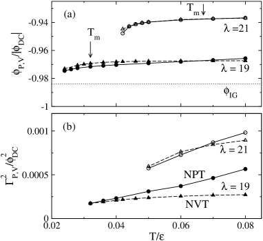
Figure 4: Average basin energy (a) and the effective Gaussian width [(b), Eq. (8)] vs temperature reduced by the LJ energy $\epsilon$ (Table 1). Open points refer to $\lambda=21$, closed points indicate $\lambda=19$. Triangles and circles refer to NVT and NPT simulations, respectively. The depth of the diamond cubic basin $\phi_{\text{DC}}$ (Table 1) is used for the energy scale. $T_{m}$ in (a) marks the melting temperature and $\phi_{\text{IG}}=\phi_{P}(T_{K}^{c})$ marks the depth of the ideal-glass minimum at which the configurational entropy $s^{c}_{P}(T)$ becomes zero ($\lambda=19$).

IV Results

IV.1 Vibrational thermodynamics

The excitation profiles $\bar{\phi}_{P,V}(T)$ and the distribution widths $\Gamma_{P,V}(T)$ for two SW potentials characterized by $\lambda=19$ and $\lambda=21$ are shown in Fig. 4. The average basin depth $\bar{\phi}_{P,V}(T)$ from simulations was fitted to the function

$$\bar{\phi}_{P,V}(T)=a_{P,V}^{(0)}+a_{P,V}^{(1)}T^{*}+a_{P,V}^{(2)}(T^{*})^{2}+b_{P,V}^{(1)}/T^{*}+b_{P,V}^{(2)}/(T^{*})^{2}$$ (16)

with $T^{*}=T/\epsilon$. The expansion coefficients in Eq. (16) are listed in Table 2. The basin depth, shown in Fig. 4 relative to the equilibrium crystalline (DC) state, changes little on this energy scale. The most interesting observation is an approximately linear increase of the effective width with temperature. This result is inconsistent with the Gaussian landscape model [Eq. (7)]. A part of the of the width increase at constant pressure comes from thermal expansion (cf. triangles with circles in Fig. 4), but there is still an increase of the effective width by a factor of nearly 2 even in constant-volume simulations. Also shown in Fig. 4 is the energy of the deepest amorphous minimum $\phi_{P}(T_{K})$, corresponding to the ideal-glass transition, measured at the Kauzmann temperature $T_{K}$ at which the configurational entropy $s_{P}^{c}(T)$ becomes zero (Table 1). This minimum lies about 820 K above the crystalline minimum, which can be compared to Stillinger’s estimate of 460 K for laboratory OTP.Stillinger (1998) The excess values are consistent with the requirement that even ideal glasses are metastable with respect to the corresponding crystals.

Table 2: Fitting coefficients in Eq. (16) for the average energy of inherent structures obtained from NPT and NVT MD simulations.

$\lambda$	Ensemble	$a_{P,V}^{(0)}$	$a_{P,V}^{(1)}$	$a_{P,V}^{(2)}$	$b_{P,V}^{(1)}$	$b_{P,V}^{(2)}$
$\lambda=19$	NPT	$-2.0013$	$0.79174$	$-2.2294$	$0.0020186$	$-2.86\times 10^{-5}$
NVT	$-1.9744$	$0.41355$	$-1.5993$	$0.001723$	$-3.03\times 10^{-5}$
$\lambda=21$	NPT	$-8.0414$	66.40	$-264.45$	0.25165	$-3.82\times 10^{-3}$
NVT	$-2.8242$	9.5033	$-35.642$	0.04262	$-7.34\times 10^{-4}$

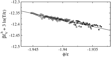
Figure 5: Basin free energy for the mSW fluid calculated in the harmonic approximation [Eq. (17)] from NPT simulations at $\lambda=19$, $\rho\sigma^{3}=0.51$, and varying temperature $T^{*}=T/\epsilon$: $0.026$ (circles), $0.028$ (squares), $0.03$ (diamonds), $0.036$ (left triangles), $0.046$ (stars). The solid line is a linear regression through the points: $\bar{\phi}_{P,V}=a_{P,V}+b_{P,V}(\phi/\epsilon)$ with $a_{P}=-23.63$ and $b_{P}=-5.80$. The NVT data, not shown here, are very close to the NPT data with the linear regression coefficients $a_{V}=-22.11$ and $b_{V}=-5.02$.

In order to gain insight into the origin of the temperature increase of $\Gamma_{P,V}(T)$ seen in Fig. 4 one needs to separate the basin free energy $f^{b}(\phi,T)$ in Eq. (6) from the enumeration function. One expects that harmonic approximation holds at low temperatures when the basin free energy can be obtained by diagonalizing the Hessian matrix at the local minimum of depth $\phi$ along the simulation trajectory

$$\beta f_{P,V}^{h}(\phi,T)=N^{-1}\langle\sum\limits_{i=1}^{3N-3}\ln\beta\hbar\omega_{i}^{P,V}\rangle_{\phi}.$$ (17)

We found, as in previous simulations,Sastry (2000); Starr et al. (2001); Sciortino (2005) that $f^{h}_{P,V}(\phi,T)$ obtained from Eq. (17) is an approximately linear function of $\phi$ (Fig. 5)

$$\beta f_{P,V}^{h}(\phi,T)+3\ln(T/\epsilon)\approx a_{P,V}+b_{P,V}(\phi/\epsilon),$$ (18)

where the linear regression coefficients are listed in the caption to Fig. 5. The basins thus become increasingly sharp on cooling, both at constant pressure and constant volume conditions. The latter observation is an agreement with the previous constant-volume simulations of SPC/E water,Starr et al. (2001) but in contrast to the opposite trend found in constant-volume simulations of BMLJ fluids.Sastry (2001)

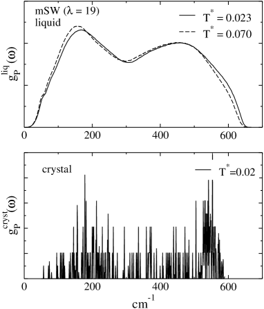
Figure 6: Density of states for mSW model ($\lambda=19$) in the liquid state at constant pressure (a) and DC crystal (b); $T^{*}=T/\epsilon$, where $\epsilon$ is the LJ energy (Tab. 1.)

The vibrational density of states (VDOS) at constant pressure, used to calculate the harmonic part of the basin free energy, is presented on Fig. 6. It was obtained by diagonalizing the Hessian of potential energy in inherent structures using LAPAC’s routine DSYEV.Anderson et al. (1992) The VDOS of the liquid phase (Fig. 6a) is continuous, with two well-defined maxima corresponding to low-frequency longitudinal and the high-frequency transverse vibrations. The VDOS shifts to higher frequencies on cooling, in agreement with Fig. 5. The crystalline VDOS was calculated for the ideal diamond cubic crystal with $N=1728$ particles. In contrast to the VDOS of the liquid phase, it has a discrete spectrum sensitive to the system size. Because of this complication, the vibrational thermodynamics of the crystal was calculated at different crystal sizes and infinite-size results were obtained by linear extrapolation of the $1/N$ dependence to $N\to\infty$.

The eigenfrequencies of the Hessian matrix $\omega_{i}$ depend weakly on temperature. This effect is caused by anharmonicity of basin vibrations which tends to soften vibrational frequencies with increasing temperature. Therefore, in order to properly calculate the harmonic free energy $f^{h}_{P,V}(T)$, we used the extrapolation of $\omega_{i}(T)$ to $T=0$. In this case, Eq. (17) with temperature-independent frequencies gives the expected value for the harmonic part of the basin internal energy

$$e^{h}_{P,V}(T)=\partial(\beta f^{h}_{P,V})/\partial\beta=3T(1-1/N).$$ (19)

Given that the basin free energy $f^{h}(\phi,T)$ is a linear function of the basin energy $\phi$ (Fig. 5), the width of the Gaussian distribution $\Gamma(T)$, obtained by fitting to the probability $P(\phi)$ function to Eq. (8), is equal to the width $\sigma$ obtained by quadratic expansion of the enumeration function around the average basin energy $\bar{\phi}_{P,V}(T)$ (second derivative of $f(\phi,T)$ in $\phi$ is zero). This conclusion is limited by the neglect of the second derivative of the anharmonic part of the basin free energy $f^{\text{anh}}(\phi,T)$ which we could not extract from our simulations. Since the Gaussian landscape precludes temperature dependence of the width, the approximately linear increase of the width of $P(\phi)$ with temperature seen in Fig. 4 can be assigned to an increase of the effective width of a non-Gaussian enumeration function fitted to a Gaussian.Matyushov (2007)

The basins of the mSW fluid are anharmonic, as is seen from the comparison of the potential energy $u(T)$ to the energy $\bar{\phi}_{P,V}(T)+(3/2)T$ (Fig. 7, lower panel). The anharmonic potential-energy part,

$$u^{\text{anh}}_{P,V}(T)=e(T)-3T-\bar{\phi}_{P,V}(T),$$ (20)

of the internal energy per particle $e(T)$ can be used to calculate the anharmonic part of the basin free energy according to the thermodynamic equation

$$\beta f^{\text{anh}}_{P,V}(T)=\int\limits_{0}^{T}u^{\text{anh}}_{P,V}(T^{\prime})d\left(\frac{1}{T^{\prime}}\right).$$ (21)

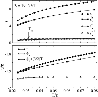
Figure 7: Total entropy $s$ (upper panel) and potential energy $u$ (lower panel) vs $T$. The entropy is split into the configurational entropy $s^{c}_{V}$, harmonic entropy $s_{V}^{h}$, and the anharmonic entropy $s^{\text{anh}}_{V}$. The potential energy (lower panel, circles) is compared to the average basin depth $\bar{\phi}_{V}$ (triangles) and the potential energy in the harmonic approximation $\bar{\phi}_{V}+(3/2)T$ (squares) ($\lambda=19$, NVT simulation).

IV.2 Configurational thermodynamics

Once the harmonic and anharmonic contributions to the basin free energy are available from Eqs. (17) and (21), the configurational entropy can be calculated by subtracting the vibrational (harmonic and anharmonic) entropy of basins from the total entropy

$$s^{c}_{P,V}(T)=s(T)-s^{h}_{P,V}(T)-s^{\text{anh}}_{P,V}(T).$$ (22)

In Eq. (21), the harmonic entropy is calculated from $T=0$ extrapolated basin frequencies as

$$s^{h}_{P,V}(T)=(N)^{-1}\sum_{i=1}^{3N-3}\left[1-\ln(\beta\hbar\omega_{i})\right],$$ (23)

and the anharmonic entropy is obtained from Eq. (21).

Thermodynamic integrationSastry (2000); Mossa et al. (2002) was employed to calculate the total entropy in Eq. (22). The excess free energy over that of the ideal gas below some reference temperature $T_{r}$ was obtained by integrating the internal energy from simulations:

$$\Delta f(T,\rho)=\Delta f(T_{r},\rho)+\int_{\beta_{r}}^{\beta}e(\rho,\beta^{\prime})d\beta^{\prime},$$ (24)

where $T_{r}$ was chosen above the critical temperature. The value $\Delta f(T_{r},\rho)$ was then obtained by isothermal expansion to the ideal gas using the equation

$$\beta_{r}\Delta f(T_{r},\rho)=\int_{0}^{\rho}\frac{d\rho^{\prime}}{\rho^{\prime}}\left(\frac{\beta_{r}P(\rho^{\prime})}{\rho^{\prime}}-1\right).$$ (25)

Finally, the free energy of the ideal gas was added to obtain the total free energy of the mSW fluid.

The excess entropy was calculated from the temperature-dependent enthalpies of the liquid and the crystal according to the relation

$$s^{\text{ex}}_{P}(T)=\Delta s^{\text{fus}}_{P}+\int_{T_{m}}^{T}\frac{dT^{\prime}}{T^{\prime}}\frac{\partial}{\partial T^{\prime}}\left(H_{\text{liq}}(T^{\prime})-H_{\text{DC}}(T^{\prime})\bigg{|}_{P}\right),$$ (26)

where $\Delta s^{\text{fus}}_{P}=2.10$ ($\lambda=19$) is the fusion entropy. The enthalpies of the liquid phase, $H_{\text{liq}}(T)$, and the DC crystal, $H_{\text{DC}}(T)$, were fitted from the simulation data to the following functions:

$$\begin{split}H_{\text{liq}}(T)&=\bar{\phi}(T)+3T+c_{2}T^{2}+c_{3}T^{3},\\ H_{\text{DC}}(T)&=-2\epsilon+3T+d_{2}T^{2}+d_{3}T^{3},\end{split}$$ (27)

where the polynomial coefficients are: $c_{2}=12.3195\epsilon^{-1}$, $c_{3}=-107.993\epsilon^{-2}$, $d_{2}=0.9352\epsilon^{-1}$, and $d_{3}=26.6414\epsilon^{-2}$. The configurational entropy, alternatively to Eq. (22), can be calculated from the configurational heat capacity

$$s^{c}_{P,V}(T)=s^{c}_{P,V}(T_{0})+\int\limits_{T_{0}}^{T}\frac{1}{T^{\prime}}\frac{d\bar{\phi}_{P,V}(T^{\prime})}{dT^{\prime}}dT^{\prime},$$ (28)

where $T_{0}$ is some temperature for which $s^{c}_{P,V}(T_{0})$ is known from the thermodynamic integration to the ideal gas. The two thermodynamic routes give identical results.

The splitting of the total liquid entropy into vibrational and configurational parts is shown in the upper panel of Fig. 7. In addition, the configurational entropy is compared in Fig. 8 to the excess entropy over the thermodynamically stable DC crystal in the temperature range between the melting temperature and the lowest temperature accessible to simulations. Also shown are the harmonic and anharmonic parts of the excess vibrational entropy. The vibrational entropy makes about half of the overall excess entropy, in a general accord with experimental evidence obtained for laboratory glass-formers.Goldstein (1976); Phillips et al. (1989); Angell (2004); Corezzi et al. (2004) The situation is somewhat similar with the excess heat capacity close to the melting point where the anharmonic vibrational part is responsible for approximately half of the excess heat capacity (harmonic excess heat capacity is identically zero). However, the fraction of the anharmonic heat capacity drops down to about 15% with lowering temperature (Fig. 8b).

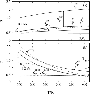
Figure 8: (a) Excess entropy of the mSW fluid over its DC crystal ($s^{\text{ex}}_{P}$) and its configurational ($s^{c}_{P,V}$) and vibrational ($s^{\text{vib}}$) components. The vibrational excess entropy is split into harmonic ($s^{\text{h}}_{P,V}$) and anharmonic ($s^{\text{anh}}_{P,V}$) parts. Configurational entropy at constant volume is shown by the dash-dotted line. (b) The splitting of the excess heat capacity $c_{P}^{\text{ex}}$ into configurational ($c_{P}^{c}$) and anharmonic vibrational ($c_{P}^{\text{anh}}$) contributions. The dashed lines in (a) and (b) refer to fits of the configurational thermodynamics to the excitations (1G) model.Matyushov and Angell (2007) The fit parameters $\{\epsilon_{0},\lambda,s_{0}\}$ are: $\{$1675 K, 787 K, 1.0$\}$. NVT simulations were done at density $\rho\sigma^{3}=0.51$ and the density changes from 0.524 at $T_{m}$ to 0.528 in NPT simulations.

We have used the data for the configurational thermodynamics from simulations to fit them to the Gaussian excitations (1G) model.Matyushov and Angell (2007) The model does not anticipate anharmonicity playing a major role in the excess thermodynamics below the melting temperature. Our focus is therefore limited to configurational thermodynamics only. As is shown in Fig. 8, the 1G models can be successfully fitted to the temperature dependence of the configurational entropy and to the high-temperature portion of the heat capacity. The model, however fails to reproduce the sharp rise of the heat capacity at the lowest temperatures accessible to simulations.

IV.3 Dynamics

The diffusivity data from simulations ($\lambda=19$) are shown by points in Fig. 9. These results are fitted to the AG relation [Eq. (1)] and to the dynamic equation of the Gaussian excitations model [Eq. (5)]. The configurational heat capacity from our simulations is used in the fit, in contrast to the previous application of Eq. (5) (Ref. Matyushov and Angell, 2007) where experimental dielectric relaxation dataRichert and Angell (1998) were fitted to Eq. (5) using the excess heat capacity from the laboratory experiment. However, for the mSW model, $c_{P}^{\text{ex}}(T)$ and $c_{P}^{c}(T)$ are off-set by almost a constant shift of anharmonic heat capacity, and the use of either of the two to fit diffusivity gives comparable results. The dashed line, almost indistinguishable from the solid line in Fig. 3, indicates the AG relation. The Vogel-Fulcher-Tammann (VFT) equation (dash-dotted line in Fig. 9) gives a less satisfactory fit. In terms of fitting the relaxation data, the AG relation is superior to both the Gaussian excitations model and the VFT equation since it involves one fitting parameter less.

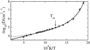
Figure 9: Fit of the diffusivity of the mSW ($\lambda=19$) fluid from simulations (hatched squares) to the AG theory [dashed line, Eq. (1)] and to the excitations model [solid line, Eq. (5)]. The dashed-dotted line refers to the Vogel-Fulcher-Tammann (VFT) equation with the VFT temperature $T_{0}$ equal to 303 K (Table 1). The dashed and solid lines are indistinguishable on the scale of the plot.

V Discussion

In discussing these results we must first recognize the sort of frustrations that are likely to accompany any effort to resolve the key problems of the glass transition by studying non-crystallizing systems using MD methods. Despite the four orders of magnitude in diffusivity that we have studied (Fig. 9) we have barely reached the onset of the “low temperature domain” (from the Stickel temperature $T_{b}$ down to $T_{g}$) in which the Adam-Gibbs equation has been tested experimentally using the excess entropy. It is in this domain that experiments show linear relations between $\log D$ and $(Ts_{P}^{\text{ex}})^{-1}$ predicted by the AG equation. Thus when, in Fig. 10, we plot our $\log D$ values against the alternative quantities $(Ts_{P}^{c})^{-1}$ and $(Ts^{\text{ex}}_{P})^{-1}$, and observe that the first is linear and the second is not, we are not able to relate the break in the $(Ts^{\text{ex}}_{P})^{-1}$ plot to the breakdown of the AG correlation at $T_{b}$ in the analysis of Richert and Angell,Richert and Angell (1998) nor to the other crossovers (Stokes-Einstein equation breakdown etc.) observed in the experimental plots at $T_{c}$.Rössler (1990); Mapes et al. (2006) The break in our $\log D$ vs $(Ts^{\text{ex}}_{P})^{-1}$ plot occurs at a quite different (much higher) temperatures, where $D$ is only $10^{-6}$ cm²s^-1, and thus must have a different origin. Whether or not there is a further break in the plot of $\log D$ vs $(Ts^{\text{ex}}_{P})^{-1}$ (or of $\log D$ vs $(Ts_{P}^{c})^{-1}$ for that matter) occurring at $T_{b}$ cannot be told from the present work, nor from any previous study.

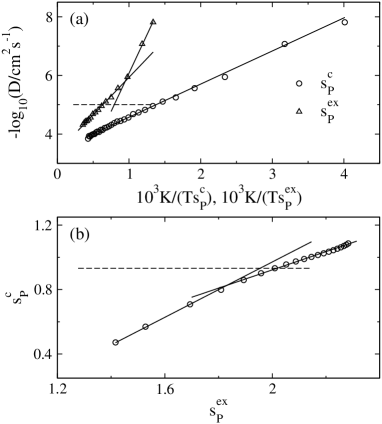
Figure 10: (a) AG plot for diffusivity using excess (triangles) and configurational (circles) entropy of the mSW fluid with $\lambda=19$. (b) $s^{\text{ex}}_{P}(T)$ vs $s^{c}_{P}(T)$ for the same system. The dashed lines represent the values of corresponding parameters at the melting temperature.

This difference between the viscosity domains explored in MD simulations of glass-formers and the low temperature domain near $T_{g}$, where so many laboratory studies are carried out, is not given adequate attention in most of the discussions of “glassy dynamics” simulation results. Notwithstanding the success of well know phenomenological models in describing the glass transition as is observed in simulation,Giovambattista et al. (2004) the fact that one is working above the much discussed crossover in the MD case and below it in the experimental range of AG equation testing, cannot be escaped. The best that can be done is to compare the slopes of the two plots with those found in the most relevant experiments. but little can be gained thereby without a better theory for the AG equation. Here we will further discuss the break in our Fig. 10 plot for diffusivities and the non-Arrhenius character of the diffusivities, and will then seek to reconcile what seems to be a conflict in dynamic and thermodynamic signatures of fragility in the present system. This will provide us with the opportunity to make a (rare) comparison of thermodynamic behavior for different potential models of simulated glass-formers.

The most complete studies of glass-former diffusivity available are for the cases of OTP,Mapes et al. (2006) SiO₂,Brebec et al. (1980) and some of the bulk metallic glasses (BMG)Faupel et al. (2003); Bartsch et al. (2006) in which data cover the range of diffusivity from water-like values down to those characteristic of liquids at their glass transition temperatures ($10^{-18}$ cm²s^-1). Only in the case of OTP is the variation of the excess entropy in the same temperature range, relative to that of the crystal, properly known. Excess entropies relative to a mixture of crystals, are known for some of the bulk metallic glass-formers.

The division of the excess entropy (and heat capacity) of the supercooled liquid into vibrational and configurational components was suggested in Goldstein’s original analysis,Goldstein (1976) where it was found that in the case of OTP almost 50% of the excess entropy was vibrational in character. Goldstein’s finding has recently been confirmed by measurements of Wang and Richert.Wang and Richert (2007) However OTP is fragile in character and the behavior of the VDOS, in Lewis-Wahnström model, is unlike that of the present system so comparison of our findings with those for OTP may not be appropriate. The bulk metallic glasses, by contrast, are more similar to the present system in their VDOS behavior (from neutron scattering studies of their quenched and annealed states,Meyer et al. (1996) but remember the observations were all made at fictive temperatures near $T_{g}$) and prove to be relatively strong in their kinetics.Faupel et al. (2003) Like the present system, their diffusivities exhibit a strong Arrhenius plot curvature in the temperature range accessible to computer simulation (thus appearing fragile in this range) in much the same way as do classical network glasses, BeF₂ and SiO₂, at high temperatures. Thus the behavior of our mSW system might be better compared with that of the BMG systems studied by Chathoth et al.Chathoth et al. (2004) and reviewed by Faupel et al.Faupel et al. (2003)

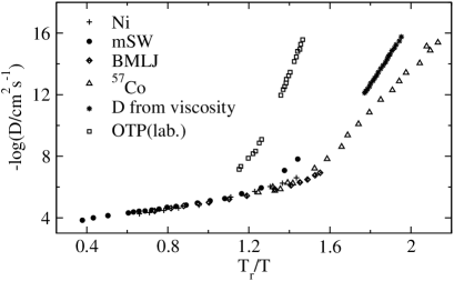
Figure 11: Diffusivity of model and laboratory glass-formers vs $T_{r}/T$, where $T_{r}$ is the temperature at which diffusivity is equal to $10^{-5}$ cm²s^-1 (the end of the Arrhenius region). Model fluids: larger component of the BMLJ liquidSastry (2001) and mSW ($\lambda=19$) fluid. Laboratory liquids: ⁵⁷Co (triangles)Bartsch et al. (2006) and Ni (pluses)Chathoth et al. (2004) tracers in Pd₄₃Cu₂₇Ni₁₀P₂₀ melt and OTP (squares).Mapes et al. (2006) Stars refer to the diffusivity of ⁵⁷Co calculated from the Stokes-Einstein equation.Bartsch et al. (2006)

In Fig. 11, we compare the diffusivities from Fig. 9 with those of various components of the bulk glass-former Pd₄₃Ni₁₀Cu₁₃P₂₀ from Refs. Chathoth et al., 2004 and Bartsch et al., 2006 after scaling by the temperature at which each system exhibits $D=10^{-5}$ cm²s^-1 (near where the deviation from Arrhenius behavior first becomes obvious). On the larger temperature scale the Ni diffusivity, like the ⁵⁷Co diffusivity of Ref. Bartsch et al., 2006 and the viscosity of Ref. Bartsch et al., 2006, all return to Arrhenius behavior with a larger slope, and the behavior appears non-fragile, approximately like glycerol. Thus the strong curvature which lead Molinero et al.Molinero et al. (2006) to conclude that mSW is very fragile, does not necessarily continue. This would rationalize what otherwise is a problem raised by the excitation profile of Fig. 4 - which is not of the form expected for a very fragile liquid according to the 1G model. This point is illustrated in Fig. 12 where the excitation profiles of the BMLJ and mSW liquids are scaled onto the same plot by the use of their Kauzmann temperatures ($T_{K}^{c}=34.35$ KSastry (2001) for BMLJ and $T_{K}=434$ K for mSW, Table 1). Unlike the more fragile cases,Matyushov and Angell (2005, 2007) which develop an S-shaped profile and exhibit phase transitions (not unlike that of silicon itself), these profiles always have positive slopes. Consistent with the difference in their diffusivity behavior seen in Fig. 11, the profile for mSW is sharper than that of the less fragile BMLJ. Figures 11 and 12 together provide the best evidence to date of the surprisingly non-fragile behavior of the much studied BMLJ system.

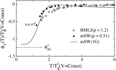
Figure 12: Excitation profiles ($\bar{\phi}_{V}(T)$) of the mSW liquid (diamonds, $\lambda=19$) vs temperature measured on the Kauzmann temperature scale; $T_{K}^{c}(V=Const)$ is from extrapolating $s_{V}^{c}(T)$ to zero. Solid line is the excitation profile obtained from the fit of 1G model to the constant-volume configurational entropy of the mSW liquid obtained by thermodynamic integration from the ideal gas reference state, and horizontal dashed line marks the position of the ideal glass basin depth. Open circles are data from the slowest effective cooling rate set of inherent structure energies from the study of Sastry et al on BMLJ at $\rho\sigma^{3}=1.213$Sastry et al. (1998) scaled using the Kauzmann temperature $T_{K}^{c}=34.35$.Sastry (2001) The level at low T in this case is not the ground state but the glassy state frozen in at this cooling rate. The sharper profile for the mSW model implies a more fragile liquid than the BMLJ model, as is also seen in the diffusivity data in Fig. 11.

A way of inducing fragile character in an atomic system spherically symmetric potential is, according to Sastry, to increase the density of BMLJ. This was shown to increase the slope of the AG plot, Fig. 10a, in the same way that is seen when the experimental data for OTP are added to the plot. We demonstrate this in Fig. 13. To show consistency, we include, in Fig. 13, the data for bulk metallic glasses, using the excess entropy data of the BMG reported by Kuno et al.Kuno et al. (2004) Although these data refer to the melting of ternary eutectic composition, we consider that the fusion enthalpy used in the entropy assessment to be valid (i.e. to contain negligible non-ideal mixing enthalpy), because it has been shown that the crystals that fuse at the eutectic are already binary compounds. The slope of the plot for the BMG diffusivities for Ni and Co, which are decoupled from the viscosity, is less than for mSW using excess entropy, but the slope for the viscosity-based data of Fig. 11 is essentially the same. The variations in slope in Fig. 13, however, are not well accounted for. Here we recall that, in Ref. Matyushov and Angell, 2007, such plots could be reduced to an all common slope using Eq. (5) of this paper.

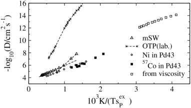
Figure 13: Comparison of AG plots of laboratory glass-formers to the simulation results of mSW ($\lambda=19$). Laboratory glass-formers: OTP (crossesMapes et al. (2006)); Ni (diamondsChathoth et al. (2004)) and ⁵⁷Co (closed squaresBartsch et al. (2006)) tracers in Pd₄₃Cu₂₇Ni₁₀P₂₀ melt. Open squares refer to the diffusivity of the same melt calculated from viscosity by using the Stokes-Einstein equation.Bartsch et al. (2006)

The analysis of the thermodynamic and relaxation data of laboratory glass-formers has allowed us to classify those liquids according to thermodynamic parameters of their configurational excitations.Matyushov and Angell (2005, 2007) The excitations model describes the thermodynamics of a supercooled liquid as an ideal gas of excitations each carrying excitation energy $\epsilon$ and entropy $s_{0}$. The energy of excitations belongs to a Gaussian manifold with the average excitation energy $\epsilon_{0}-2x(T)\lambda$ ($x(T)$ is the population of the excited state) and the variance $2T\lambda$. This representation is in fact equivalent to an ensemble of excitations with mean-field attractions. When the laboratory data for fragile liquids are fitted to the 1G model, the excitation parameters show universality when the energies are scaled with the Kauzmann temperature. In these reduced units, the excitation entropy $s_{0}$ becomes the only relevant parameter determining fragility as shown in Fig. 14 where the data are plotted against the steepness fragility index:Wang et al. (2006)

$$\frac{\epsilon_{0}}{2T_{K}}\simeq\frac{\lambda}{T_{K}}\simeq s_{0}.$$ (29)

This universality does not hold for liquids of intermediate fragility (intermediate liquids). Noteworthy is a much smaller width parameter $\lambda$ for intermediate liquids compared to fragile liquids (Fig. 14).

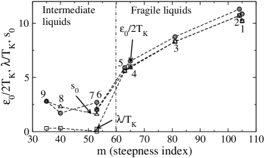
Figure 14: Excitation energy $\epsilon_{0}$, the trapping energy parameter $\lambda$, and the excitation entropy $s_{0}$ of some laboratory glass-formers. The energy parameters are scaled with the experimental Kauzmann temperature $T_{K}$. The parameters obtained by fitting the excitation 1G model to experimental excess thermodynamic data are plotted against the steepness fragility parameter $m$.Angell (1995) The fragility number $m\simeq 60$ separates fragile from intermediate liquids (dash-dotted line). The numbers in the plot indicate: toluene (1), D,L-propene carbonate (2), OTP (3), 2-methyltetrahydrofurane (4), salol (5), 3-bromopentane (6), glycerol (7), selenium (8), and $n$-propanol (9). For selenim, the steepness index of $m=40$ calculated in Ref. Wang et al., 2006 was used.

The current simulations of the mSW liquid generally support the basic assumptions incorporated in the development of the excitations model of low-temperature glass-formers,Matyushov and Angell (2005, 2007) although, as for the comparison to laboratory data, the MD simulations probe the temperature range much higher than the one anticipated in the theory development ($T_{g}\leq T\leq T_{b}$). Nevertheless, some conclusions can be drawn. The 1G model neglects the temperature dependence of the excitation entropy and thus the anharmonicity effects. Anharmonic vibrations are significant in the potential energy landscape of the mSW model at high temperatures, but their contribution to the excess heat capacity drops to about $\simeq 15$ % in the lowest portion of the temperature range studied here. Therefore, the assumption of the temperature-independent entropy of elementary excitations might be a good first-order approximation in applications of the model to data at low temperatures close to $T_{g}$.

The most significant ingredient of the excitations model requiring testing on available data is the anticipated temperature dependence of the effective Gaussian width of the distribution of basin energies. The temperature-dependent width is introduced into the model to account for an effectively non-Gaussian landscape probed by the system when exploring deeper basins with lowering temperature. An exact non-Gaussian landscape model recently developed by one of usMatyushov (2007) has taught us that this temperature dependence can be quite complex such that a linear scaling probably applies only to a limited range of temperatures. Even though, in the range of temperatures studied by our simulations, the effective width scales linearly with temperature for both constant-volume and constant-pressure ensembles (Fig. 4). Unfortunately, the present simulations do not allow access to the lower portion of the landscape, and deviations from gaussianity observed in some recent simulationsMoreno et al. (2006); Matyushov (2007) are not pronounced in the enumeration function $\omega(\phi)$.