Quantum Zeno dynamics and quantum Zeno subspaces

Abstract

A quantum Zeno dynamics can be obtained by means of frequent measurements, frequent unitary kicks or a strong continuous coupling and yields a partition of the total Hilbert space into quantum Zeno subspaces, among which any transition is hindered. We focus on the “continuous” version of the quantum Zeno effect and look at several interesting examples. We first analyze these examples in practical terms, towards applications, then propose a novel experiment.

1 Introduction

The quantum Zeno effect is intertwined with the name of George Sudarshan, who cast the problem in a rigorous mathematical framework and proposed the classical allusion to the sophist philosopher in a seminal article written in collaboration with Baidyanaith Misra in 1977 [1]. Somewhat curiously, the most remarkable practical application of the quantum Zeno effect consists in reducing (and eventually suppressing) decoherence and dissipation, which are other issues in which George Sudarshan was a protagonist, by establishing a firm physical and mathematical description that is known nowadays as the Gorini-Kossakowski-Sudarshan-Lindblad equation [2]. The aim of this article is to illustrate the main features of the quantum Zeno effect (QZE), clarify what is a quantum Zeno dynamics, discuss examples and recent experiments and propose applications.

The quantum Zeno effect has an interesting history. It was first understood by von Neumann [3], who proved that any given quantum state $\phi$ can be “steered” into any other state $\psi$, by applying a suitable series of measurements. If $\phi$ and $\psi$ coincide (modulo a phase factor), the evolution yields, in modern language, a quantum Zeno effect. After 35 years (!) Beskow and Nilsson [4] considered a particle in a bubble chamber (thought of as an apparatus that “continuously checks” whether the particle has decayed) and wondered whether this “measurement” mechanism can hinder decay. This interesting intuition was then reconsidered by other authors, both from a physical [5, 6] and more genuinely mathematical perspective [7]. Notice that a rigorous formulation hinges upon difficult mathematical issues [8], most of which are yet unsolved [9].

It was not until 1988 that Cook realized that the quantum Zeno effect (not a “paradox” as people tended to regard it) could be tested on oscillating (two- or three-level) systems [10]. This proposal deviated from the original framework, that dealt with bona fide unstable systems [4, 1], but was nonetheless an interesting and concrete idea, that led to a beautiful experimental test a few years later, performed by Itano and collaborators [11]. The debate that followed [12] motivated novel experimental tests, involving diverse physical systems, such as photon polarization, chiral molecules and ions [13] and very recently Bose-Einstein condensates [14] and cavity QED [15]. New experiments have been proposed with neutron spin [16].

The presence of a short-time quadratic (Zeno) region for a bona fide unstable quantum mechanical system (particle tunnelling out of a confining potential) was experimentally confirmed by Raizen and collaborators in 1997 [17]. A few years later, the same group demonstrated the Zeno effect (hindered evolution by frequent measurements) [18]. This experiment also proved the occurrence of the curious inverse (or anti) Zeno effect (IZE) [19, 20], first suggested in 1983 (!), according to which the evolution can be accelerated if the measurements are frequent, but not too frequent. The IZE has remarkable links with chaos and dynamical localization [21].

The QZE arises as a straightforward consequence of general features of the Schrödinger equation, that yield quadratic behavior of the survival probability at short times [22, 23]. It is usually understood as the hindrance of the dynamics out of the intial state due to frequent von Neumann measurements. Nowadays, in view of possible applications, this picture appears too restrictive in two respects. First, the QZE does not necessarily freeze the dynamics. On the contrary, for frequent projections onto a multidimensional subspace, the system can evolve away from its initial state, although it remains in the “Zeno subspace” defined by the measurement [24]. The resulting constrained evolution is called “quantum Zeno dynamics” [25]. Second, the QZE can be reformulated in terms of a “continuous coupling” [23], without making use of projection operators and non-unitary dynamics, obtaining the same physical effects. We emphasize that the idea of a continuous formulation of the QZE is not new [26, 6], but has appeared in the literature in different contexts and at different times. These two observations will enable us to focus on possible interesting applications and novel experimental proposals.

This article is organized as follows. We start by reviewing some notions related to the (familiar) “pulsed” formulation of the Zeno effect in Sec. 2. We then summarize the celebrated Misra and Sudarshan theorem in Sec. 3. This theorem is generalized in Sec. 4, in order to accommodate nonselective measurements. We briefly introduce the “kicked” version of the QZE in Sec. 5 and the continuous formulation in Sec. 6. The three procedures (pulsed, kicked and continuous QZE) are compared in Sec. 7, where their physical equivalence is discussed. We then look at several elementary but relevant examples in Secs. 8-10. This is a central part of the article, where a new experiment is proposed. We conclude with a few comments in Sec. 11.

2 Preliminaries: the “pulsed” formulation

We start off by giving an elementary introduction to the QZE, in its most familiar formulation, in terms of von Neumann measurements represented by one-dimensional projections. Let $H$ be the total Hamiltonian of a quantum system Q and $|\psi_{0}\rangle$ its initial state at $t=0$. The survival amplitude and probability in state $|\psi_{0}\rangle$ at time time $t$ read ($\hbar=1$)

$${\mathcal{A}}(t) = \langle\psi_{0}|e^{-iHt}|\psi_{0}\rangle,$$ (1)

$$p(t) = |{\mathcal{A}}(t)|^{2}=|\langle\psi_{0}|e^{-iHt}|\psi_{0}\rangle|^{2}$$ (2)

and a short-time expansion yields a quadratic behavior

$$p(t) \sim 1-t^{2}/\tau_{\mathrm{Z}}^{2},$$ (3)

$$\tau_{\mathrm{Z}}^{-2} \equiv \langle\psi_{0}|H^{2}|\psi_{0}\rangle-\langle\psi_{0}|H|\psi_{0}\rangle^{2},$$ (4)

where $\tau_{\mathrm{Z}}$ is the Zeno time [27]. Observe that if the Hamiltonian is divided into a free and an (off-diagonal) interaction parts

$$H=H_{0}+H_{\mathrm{int}},$$

$$H_{0}|\psi_{0}\rangle=\omega_{0}|\psi_{0}\rangle,$$

$$\langle\psi_{0}|H_{\mathrm{int}}|\psi_{0}\rangle=0,$$ (5)

the Zeno time reads

$$\tau_{\mathrm{Z}}^{-2}=\langle\psi_{0}|H_{\mathrm{int}}^{2}|\psi_{0}\rangle$$ (6)

and depends only on the interaction Hamiltonian.

Let us now show how frequent projective measurements can hinder evolution away from the initial state. Perform $N$ measurements at time intervals $\tau=t/N$, in order to check whether the system is still in its initial state $|\psi_{0}\rangle$. The survival probability $p^{(N)}(t)$ at time $t$ reads

$$p^{(N)}(t)=p(\tau)^{N}=p\left(t/N\right)^{N}\sim\exp\left(-t^{2}/\tau_{\mathrm{Z}}^{2}N\right)\stackrel{{\scriptstyle N\rightarrow\infty}}{{\longrightarrow}}1.$$ (7)

For large $N$ the evolution is slowed down and in the $N\to\infty$ limit the evolution is completely hindered. Notice that the survival probability after $N$ pulsed measurements ($t=N\tau$) is interpolated by an exponential law [20]

$$p^{(N)}(t)=p(\tau)^{N}=\exp(N\log p(\tau))=\exp(-\gamma_{\mathrm{eff}}(\tau)t),$$ (8)

with an effective decay rate

$$\gamma_{\mathrm{eff}}(\tau)\equiv-\frac{1}{\tau}\log p(\tau)=-\frac{2}{\tau}\log|{\mathcal{A}}(\tau)|=-\frac{2}{\tau}\mathrm{\,Re\,}[\log{\mathcal{A}}(\tau)]\geq 0\;.$$ (9)

For $\tau\to 0$ ($N\to\infty$) one gets $p(\tau)\sim\exp(-\tau^{2}/\tau_{\mathrm{Z}}^{2})$, whence

$$\gamma_{\mathrm{eff}}(\tau)\sim\tau/\tau_{\mathrm{Z}}^{2},\qquad\tau\to 0.$$ (10)

The Zeno evolution for “pulsed” measurements is pictorially represented in Figure 1.

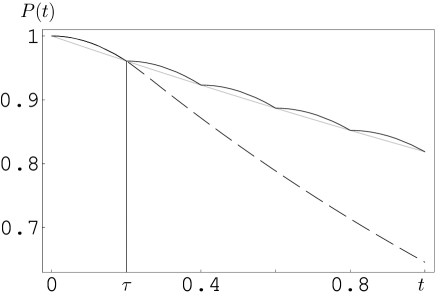
Figure 1: Quantum Zeno effect in the “pulsed” formulation. The dashed (full) line is the survival probability without (with) measurements. The gray line is the interpolating exponential (8). The units on the abscissae are arbitrarily chosen for illustrative purposes.

3 Misra and Sudarshan’s theorem

The formulation of the previous section is very intuitive and does not rest on a firm mathematical ground. The existence of the moments of the Hamiltonian and the convergence of the expansions are all taken for granted and subtle field-theoretical issues related to the Fermi golden rule [28] are not considered [29, 27].

The formulation by Misra and Sudarshan consists in a theorem that requires a few preliminary notions. We first introduce incomplete measurements, represented by multidimensional projections, by applying the von Neumann-Lüders [3, 30] formulation in terms of projection operators and adopting some definitions given by Schwinger [31] (but see also Peres [32]). We will say that a measurement is “incomplete” if some outcomes are lumped together. This happens, for example, if the experimental equipment has insufficient resolution (and in this sense the information on the measured observable is incomplete). The projection operator $P$, that selects a particular lump, is therefore multidimensional.

Let ${\cal H}$ be the Hilbert space of system Q and let the evolution be described by the unitary operator $U(t)=\exp(-iHt)$, where $H$ is a time-independent lower-bounded Hamiltonian. Let $P$ be a projection operator and $\textrm{Ran}P={\mathcal{H}}_{P}$ its range, with $\mathrm{dim}{\mathcal{H}}_{P}=\mathrm{Tr}P=s\leq\infty$ (not necessarily finite dimensional). We assume that the initial density matrix $\rho_{0}$ of system Q belongs to ${\cal H}_{P}$:

$$\rho_{0}=P\rho_{0}P,\qquad\mathrm{Tr}[\rho_{0}P]=1.$$ (11)

Under the sole action of the Hamiltonian $H$ (no measurements), the state at time $t$ reads

$$\rho(t)=U(t)\rho_{0}U^{\dagger}(t)$$ (12)

and the survival probability (namely the probability that the system is still in ${\cal H}_{P}$) at time $t$ reads

$$p(t)=\mathrm{Tr}\left[U(t)\rho_{0}U^{\dagger}(t)P\right].$$ (13)

No distinction is made between one- and multi-dimensional projections.

The above evolution is “undisturbed:” Q evolves under the sole action of its Hamiltonian for a time $t$, without undergoing any measurement process. We now perform a selective measurement at time $\tau$, in order to check whether Q has “survived” inside ${\cal H}_{P}$. By “selective”, we mean that we filter out the survived component and stop the other ones. (Think for instance of decomposing a spin in a Stern-Gerlach setup and absorbing away the unwanted components.) The state of Q changes into

$$\rho_{0}\rightarrow\rho(\tau)=\frac{PU(\tau)\rho_{0}U^{\dagger}(\tau)P}{p(\tau)},$$ (14)

where

$$p(\tau)=\mathrm{Tr}\left[U(\tau)\rho_{0}U^{\dagger}(\tau)P\right]=\mathrm{Tr}\left[V(\tau)\rho_{0}V^{\dagger}(\tau)\right],\qquad V(\tau)\equiv PU(\tau)P$$ (15)

is the survival probability in ${\cal H}_{P}$. The QZE is the following. We prepare Q in the initial state $\rho_{0}$ at time 0 and perform a series of (selective) $P$-observations at time intervals $\tau=t/N$ (by this we mean that Q is found in ${\mathcal{H}}_{P}$ at every step). The state at time $t$ reads

$$\rho^{(N)}(t)=\frac{V_{N}(t)\rho_{0}V_{N}^{\dagger}(t)}{p^{(N)}(t)},\qquad V_{N}(t)=\left[V\left(\frac{t}{N}\right)\right]^{N},$$ (16)

where

$$p^{(N)}(t)=\mathrm{Tr}\left[V_{N}(t)\rho_{0}V_{N}^{\dagger}(t)\right]$$ (17)

is the survival probability in ${\cal H}_{P}$. Equations (16)-(17) are the formal statement of the QZE, according to which very frequent observations modify the dynamics of the quantum system: under general conditions, if $N$ is sufficiently large, transitions outside ${\cal H}_{P}$ are inhibited.

The $N\rightarrow\infty$ limit requires some technical hypotheses: assume that the strong limit

$${\mathcal{V}}(t)\equiv\lim_{N\rightarrow\infty}V_{N}(t)$$ (18)

exists $\forall t>0$. The final state of Q is then

$$\rho(t)=\lim_{N\to\infty}\rho^{(N)}(t)={\mathcal{V}}(t)\rho_{0}{\mathcal{V}}^{\dagger}(t)$$ (19)

and the survival probability in ${\mathcal{H}}_{P}$ is

$${\mathcal{P}}(t)\equiv\lim_{N\rightarrow\infty}p^{(N)}(t)=\mathrm{Tr}\left[{\mathcal{V}}(t)\rho_{0}{\mathcal{V}}^{\dagger}(t)\right].$$ (20)

By assuming the strong continuity of ${\mathcal{V}}(t)$ at $t=0$

$$\lim_{t\rightarrow 0^{+}}{\mathcal{V}}(t)=P,$$ (21)

Misra and Sudarshan proved that under general conditions the operators ${\mathcal{V}}(t)$ exist $\forall t\in\mathbb{R}$ and form a semigroup. Moreover, by time-reversal invariance

$${\mathcal{V}}^{\dagger}(t)={\mathcal{V}}(-t),$$ (22)

one gets ${\mathcal{V}}^{\dagger}(t){\mathcal{V}}(t)=P$. This implies, by (11), that

$${\mathcal{P}}(t)=\mathrm{Tr}\left[\rho_{0}{\mathcal{V}}^{\dagger}(t){\mathcal{V}}(t)\right]=\mathrm{Tr}\left[\rho_{0}P\right]=1.$$ (23)

If the particle is very frequently observed, in order to check whether it has survived inside ${\mathcal{H}}_{P}$, it will never make a transition to ${\mathcal{H}}_{P}^{\perp}$. In general, if $N$ is sufficiently large in (16)-(17), transitions outside ${\cal H}_{P}$ are inhibited. However, if $N$ is not too large the system can display an inverse Zeno effect [19, 20], by which decay is accelerated. Both effects have been demonstrated [18]. We will not elaborate on this here.

A few comments are in order. Notice that the dynamics (16)-(17) is not reversible. On the other hand, the dynamics in the $N\to\infty$ limit is often time reversible [24] (although, in general, the operators ${\mathcal{V}}(t)$ form a semigroup). Observe also that the Misra and Sudarshan theorem does not state that the system remains in its initial state, after the series of very frequent measurements. Rather, the system evolves in the subspace ${\mathcal{H}}_{P}$, instead of evolving “undisturbed” in the total Hilbert space ${\mathcal{H}}$. The limiting Zeno dynamics within ${\mathcal{H}}_{P}$ is governed by (18), which can be a unitary group. Therefore, starting from the dynamics (16), which is irreversible and probability-nonconserving, one may end up with a fully unitary evolution. Unitarity is recovered in the limit. The features of this evolution in some simple cases will be the object study of the following sections. We anticipate that if ${\mathcal{H}}_{P}\subset D(H)$, the domain of the Hamiltonian $H$, the limiting time evolution has the explicit form

$${\mathcal{V}}(t)=P\exp(-iPHPt),$$ (24)

namely ${\mathcal{V}}(t)$ is unitary within ${\mathcal{H}}_{P}$ and is generated by the self-adjoint Hamiltonian $PHP$: reversibility is recovered in the $N\to\infty$ limit. In particular, Eq. (24) is always valid for bounded Hamiltonian, since $D(H)={\mathcal{H}}$. In more general cases (infinite dimensional projectors, $s=\mathrm{dim}{\mathcal{H}}_{P}=\infty$, unbounded $H$) one can always formally write the limiting evolution in the form (24), but has to define the meaning of $PHP$. In such a case one has to study the self-adjointness of the formal limiting Hamiltonian $PHP$ [7, 24, 8, 9].

4 Extension of the Misra and Sudarshan theorem: The quantum Zeno subspaces

We now consider more general measurements and extend the Misra and Sudarshan theorem in order to accommodate multiple projectors. We will say that a measurement is “nonselective” [31] if the measuring apparatus does not “select” the different outcomes, so that all the “branch waves” undergo the whole Zeno dynamics. In other words, a nonselective measurement destroys the phase correlations between different branch waves, provoking the transition from a pure state to a mixture. Let

$$\{P_{n}\}_{n},\qquad P_{n}P_{m}=\delta_{mn}P_{n},\qquad\sum_{n}P_{n}=1,$$ (25)

be a (countable) collection of projection operators and $\mathrm{Ran}P_{n}={\mathcal{H}}_{P_{n}}$ the relative subspaces. This induces a partition on the total Hilbert space

$${\mathcal{H}}=\bigoplus_{n}{\mathcal{H}}_{P_{n}}.$$ (26)

Consider the associated nonselective measurement described by the superoperator [3, 30]

$$\hat{P}\rho=\sum_{n}P_{n}\rho P_{n}.$$ (27)

The free evolution reads

$$\hat{U}_{t}\rho_{0}=U(t)\rho_{0}U^{\dagger}(t),\qquad U(t)=\exp(-iHt)$$ (28)

and the Zeno evolution after $N$ measurements in a time $t$ is governed by the superoperator

$$\hat{V}^{(N)}_{t}=\hat{P}\left(\hat{U}\left(t/N\right)\hat{P}\right)^{N-1}.$$ (29)

This yields the evolution

$$\rho(t)=\hat{V}^{(N)}_{t}\rho_{0}=\sum_{n_{1},\dots,n_{N}}V_{n_{1}\dots n_{N}}^{(N)}(t)\;\rho_{0}\;V_{n_{1}\dots n_{N}}^{(N)\dagger}(t),$$ (30)

where

$$V_{n_{1}\dots n_{N}}^{(N)}(t)=P_{n_{N}}U\left(t/N\right)P_{n_{N-1}}\cdots P_{n_{2}}U\left(t/N\right)P_{n_{1}},$$ (31)

which should be compared to Eq. (16). We follow Misra and Sudarshan [1] and assume, as in Sec. 3, the existence of the strong limits ($t\in\mathbb{R}$)

$${\mathcal{V}}_{n}(t)=\lim_{N\to\infty}V_{n\dots n}^{(N)}(t),\qquad\lim_{t\rightarrow 0}{\mathcal{V}}_{n}(t)=P_{n},\quad\forall n\ .$$ (32)

Then ${\mathcal{V}}_{n}(t)$ form a semigroup for every $n$ and

$${\mathcal{V}}_{n}^{\dagger}(t){\mathcal{V}}_{n}(t)=P_{n}.$$ (33)

Moreover, one can show that

$$\lim_{N\to\infty}V_{n\dots n^{\prime}\dots}^{(N)}(t)=0,\qquad\mathrm{for}\quad n^{\prime}\neq n,$$ (34)

strongly. Notice that, for any finite $N$, the off-diagonal operators (31) are in general nonvanishing, i.e. $V_{n\dots n^{\prime}\dots}^{(N)}(t)\neq 0$ for $n^{\prime}\neq n$. It is only in the limit (34) that these operators vanish. This is because $U\left(t/N\right)$ provokes transitions among different subspaces ${\mathcal{H}}_{P_{n}}$. By Eqs. (32)-(34) the final state is

$$\rho(t)=\hat{\mathcal{V}}_{t}\rho_{0}=\sum_{n}{\mathcal{V}}_{n}(t)\rho_{0}{\mathcal{V}}_{n}^{\dagger}(t),\quad\mathrm{with}\quad\sum_{n}{\mathcal{V}}_{n}^{\dagger}(t){\mathcal{V}}_{n}(t)=\sum_{n}P_{n}=1.\;\;$$ (35)

The components ${\mathcal{V}}_{n}(t)\rho_{0}{\mathcal{V}}_{n}^{\dagger}(t)$ make up a block diagonal matrix: the initial density matrix is reduced to a mixture and any interference between different subspaces ${\mathcal{H}}_{P_{n}}$ is destroyed (complete decoherence). In conclusion,

$$p_{n}(t)=\mathrm{Tr}\left[\rho(t)P_{n}\right]=\mathrm{Tr}\left[\rho_{0}P_{n}\right]=p_{n}(0),\quad\forall n.$$ (36)

Probability is conserved in each subspace and no probability “leakage” between any two subspaces is possible: the total Hilbert space splits into invariant subspaces and the different components of the wave function (or density matrix) evolve independently within each sector. One can think of the total Hilbert space as the shell of a tortoise, each invariant subspace being one of the scales. Motion among different scales is impossible. (See Fig. 2 in the following.)

If ${\mathcal{H}}_{P_{n}}\subset D(H)$, then the limiting evolution operator ${\mathcal{V}}_{n}(t)$ (32) within the subspace ${\mathcal{H}}_{P_{n}}$ has the form (24),

$${\mathcal{V}}_{n}(t)=P_{n}\exp(-iP_{n}HP_{n}t),$$ (37)

$P_{n}HP_{n}$ is bounded and self-adjoint and ${\mathcal{V}}_{n}(t)$ is unitary in ${\mathcal{H}}_{P_{n}}$. Precautions are necessary in more general cases, as mentioned after Eq. (24).

The result (23) is reobtained when $p_{n}(0)=1$ for some $n$, in (36): the initial state is then in one of the invariant subspaces and the survival probability in that subspace remains unity. In conclusion, when the necessary care is taken for mathematical rigor and subtleties, the Zeno evolution can be written

$$\rho(t) = \hat{\mathcal{V}}_{t}\rho_{0}=\sum_{n}{\mathcal{V}}_{n}(t)\rho_{0}{\mathcal{V}}_{n}^{\dagger}(t),$$ (38)

$${\mathcal{V}}_{n}(t) = P_{n}\exp(-iH_{\mathrm{Z}}t)$$ (39)

where

$$H_{\mathrm{Z}}=\hat{P}H=\sum_{n}P_{n}HP_{n}$$ (40)

is the “Zeno” Hamiltonian.

5 Unitary kicks

The formulation of the preceding section hinges upon projections à la von Neumann. Projections are instantaneous processes, yielding the collapse of the wave function (an ultimately nonunitary process). However, one can obtain the QZE without making use of nonunitary evolutions. In this section we further elaborate on this issue, obtaining the QZE by means of a generic sequence of frequent instantaneous unitary processes. We will only give the main results, as additional details and a complete proof, which is related to von Neumann’s ergodic theorem [33], can be found in [34].

Consider the dynamics of a quantum system Q undergoing $N$ “kicks” $U_{\mathrm{kick}}$ (instantaneous unitary transformations) in a time interval $t$

$$U_{N}(t)=\left[U_{\mathrm{kick}}U\left(\frac{t}{N}\right)\right]^{N}.$$ (41)

In the large $N$ limit, since the dominant contribution is $U_{\mathrm{kick}}^{N}$, one considers the sequence of unitary operators

$$V_{N}(t)=U_{\mathrm{kick}}^{\dagger N}U_{N}(t)=U_{\mathrm{kick}}^{\dagger N}\left[U_{\mathrm{kick}}U\left(\frac{t}{N}\right)\right]^{N}$$ (42)

and its limit

$${\mathcal{U}}(t)\equiv\lim_{N\to\infty}V_{N}(t).$$ (43)

One can show that

$${\mathcal{U}}(t)=\exp(-iH_{\mathrm{Z}}t),$$ (44)

where

$$H_{\mathrm{Z}}=\hat{P}H=\sum_{n}P_{n}HP_{n}$$ (45)

is the Zeno Hamiltonian, $P_{n}$ being the spectral projections of $U_{\mathrm{kick}}$

$$U_{\mathrm{kick}}=\sum_{n}e^{-i\lambda_{n}}P_{n}.\quad(e^{-i\lambda_{n}}\neq e^{-i\lambda_{l}},\;\mbox{for}\;n\neq l).$$ (46)

In conclusion

$$U_{N}(t) \sim U_{\mathrm{kick}}^{N}{\mathcal{U}}(t)=U_{\mathrm{kick}}^{N}\exp(-iH_{\mathrm{Z}}t)$$ (47)

$$= \exp\left(-i\sum_{n}N\lambda_{n}P_{n}+P_{n}HP_{n}t\right).$$ (48)

The unitary evolution (41) yields therefore a Zeno effect and a partition of the Hilbert space into Zeno subspaces, like in the case of repeated projective measurements discussed in the previous section. The appearance of the Zeno subspaces is a direct consequence of the wildly oscillating phases between different eigenspaces of the kick.

6 Continuous coupling

The formulation of the preceding sections hinges upon instantaneous processes, that can be unitary or nonunitary. However, the main features of the QZE can be obtained by making use of a continuous coupling, when the external system takes a sort of steady “gaze” at the system of interest. The mathematical formulation of this idea is contained in a theorem [25] on the (large-$K$) dynamical evolution governed by a generic Hamiltonian of the type

$$H_{K}=H+KH_{\mathrm{c}},$$ (49)

which again need not describe a bona fide measurement process. $H$ is the Hamiltonian of the quantum system investigated and $H_{\mathrm{c}}$ can be viewed as an “additional” interaction Hamiltonian performing the “measurement.” $K$ is a coupling constant.

Consider the time evolution operator

$$U_{K}(t)=\exp(-iH_{K}t).$$ (50)

In the “infinitely strong coupling” (“infinitely quick detector”) limit $K\to\infty$, the dominant contribution is $\exp(-iKH_{\mathrm{c}}t)$. One therefore considers the limiting evolution operator

$${\mathcal{U}}(t)=\lim_{K\to\infty}\exp(iKH_{\mathrm{c}}t)\,U_{K}(t),$$ (51)

that can be shown to have the form

$${\mathcal{U}}(t)=\exp(-iH_{\mathrm{Z}}t),$$ (52)

where

$$H_{\mathrm{Z}}=\hat{P}H=\sum_{n}P_{n}HP_{n}$$ (53)

is the Zeno Hamiltonian, $P_{n}$ being the eigenprojection of $H_{\mathrm{c}}$ belonging to the eigenvalue $\eta_{n}$

$$H_{\mathrm{c}}=\sum_{n}\eta_{n}P_{n},\qquad(\eta_{n}\neq\eta_{m},\quad\mbox{for}\;n\neq m)\ .$$ (54)

This is formally identical to (40) and (45). In conclusion, the limiting evolution operator is

$$U_{K}(t) \sim \exp(-iKH_{\mathrm{c}}t)\,{\mathcal{U}}(t)$$ (55)

$$= \exp\left(-i\sum_{n}Kt\eta_{n}P_{n}+P_{n}HP_{n}t\right),$$ (56)

whose block-diagonal structure is explicit. Compare with (48). The above statements can be proved by making use of the adiabatic theorem [35].

7 A few comments on the three formulations

The three different formulations of QZE summarized in the previous sections are physically equivalent and the analogy among them can be pushed very far [34].

After all, a projection à la von Neumann is a handy way to “summarize” the complicated physical processes that take place during a quantum measurement. A measurement process is performed by an external (macroscopic) apparatus and involves dissipative effects (an interaction and an exchange of energy with and often a flow of probability towards the environment). The external system performing the observation need not be a bona fide detection system, namely a system that “clicks” or is endowed with a pointer. For instance, a spontaneous emission process is often a very effective measurement process, for it is irreversible and leads to an entanglement of the state of the system (the emitting atom or molecule) with the state of the apparatus (the electromagnetic field). The von Neumann rules arise when one traces away the photonic state and is left with an incoherent superposition of atomic states. However, it is clear that the main features of the Zeno effects are still present if one formulates the measurement process in more realistic terms, introducing a physical apparatus, a Hamiltonian and a suitable interaction with the system undergoing the measurement. It goes without saying that one can still make use of projection operators, if such a description turns out to be simpler and more economic (Occam’s razor).

A comparison of the three Zeno procedures outlined in the three preceding sections suggests that the continuous version might be the most effective strategy against decoherence [36]. We shall therefore look at some simple examples that yield a quantum Zeno subspace by making use of a strong continuous coupling. As already emphasized, the idea that a strong continuous coupling to an external apparatus can yield a Zeno-like behavior has often been proposed in the literature of the last two decades [26, 23]. The novelty in this context is the appearance of effective superselection rules that are de facto equivalent to the celebrated “W³” ones [37], but turn out to be a mere consequence of the Zeno dynamics. This remarkable aspect is reminiscent of some results on “classical” observables [38], the semiclassical limit [39] and quantum measurement theory [40, 31]. The appearance of a superselection rule in the Hilbert space of the system is pictorially represented in Fig. 2. We conclude by observing that the algebra of observables in the Zeno subspaces is in itself an open problem and a topic worth investigating [41].

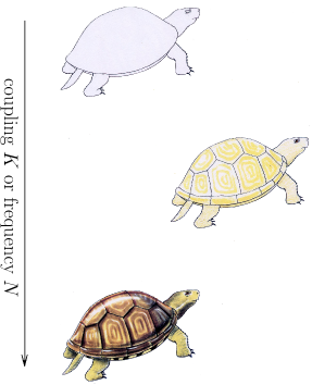
Figure 2: The Hilbert space of the system: a dynamical superselection rule appears as the coupling $K$ to the apparatus or the frequency $N$ of measurements is increased.

8 Example: three level system

Let us now look at some simple examples, involving only finite-dimensional Hilbert spaces. Let us first consider the experiment schematically shown in Fig. 3. Two levels 1 and 2 are Rabi coupled and frequent pulses rapidly sweep the population from level 2 to level 3. If the decay rate $\Gamma$ out of level 3 is fast enough, this can be viewed as a very efficient measurement procedure and QZE takes place. This is the scheme adopted by Itano and collaborators in their celebrated experiment [11]. Observe that in Fig. 3 one implicitly assumes $\pi/2$-pulses; on the other hand, if one makes the pulses extremely frequent and accordingly less intense (technically, one rescales the Hamiltonian [34]), one gets a situation similar to that shown in Fig. 4. In this sense, both “pulsed” and “continuous” measurements are physically equivalent in that they both yield QZE. This observation motivated a recent experiment performed at MIT with a BEC [14].

Consider now the scheme shown in Fig. 4, that describes a three-level system undergoing two different Rabi oscillations and coupled to the photon field. Photons drain the population away from level 3 (towards some other level not shown in the figure), so that if one restricts one’s attention to the three atomic levels 1, 2 and 3, the effective Hamiltonian in the Markovian approximation reads $(\hbar=1)$

$$H=\frac{\omega}{2}(|1\rangle\langle 2|+|2\rangle\langle 1|)+\frac{\omega^{\prime}}{2}(|2\rangle\langle 3|+|3\rangle\langle 2|)-i\frac{\Gamma}{2}|3\rangle\langle 3|=\frac{1}{2}\pmatrix{0&\omega&0\cr\omega&0&\omega^{\prime}\cr 0&\omega^{\prime}&-i\Gamma},$$ (57)

where

$$\langle 1|=(1,0,0),\quad\langle 2|=(0,1,0),\quad\langle 3|=(0,0,1).$$ (58)

This is the effective Hamiltonian that better describes the MIT experiment [14]. Once a $\Gamma$-photon has been emitted, the atom recoils and leaves the condensate. Here and in the following we will oversimplify the analysis in order to focus on the main ideas.

The Hamiltonian (57) is not Hermitian and probability is not conserved (the photon field has been traced out). Let us prepare the system in state $|1\rangle$ and let

$$p_{1}(t)=|\langle 1|e^{-iHt}|1\rangle|^{2}$$ (59)

be the survival probability. This is our key quantity, that can be studied in different regimes.

Figure 3: “Pulsed” QZE, as in the experiment by Itano et al [11].

Figure 4: “Continuous” observation, as in the experiment performed at MIT with a BEC [14].

The main idea is that a larger coupling to the photon field (via $\omega^{\prime}$ and $\Gamma$) yields a more effective “continuous” observation of the population of level 2 (and therefore of level 1), due to a quicker response of the environment/detection system. As a consequence, the evolution is slower and one obtains QZE. We assume [14]

$$\Gamma,\omega^{\prime}\gg\omega,$$ (60)

which enables one to adopt the effective description of Fig. 5: Consider only the two levels

$$\langle 1|=(1,0),\quad\langle 2|=(0,1),$$ (61)

with the effective Hamiltonian

$$H_{{\rm eff}}=\frac{1}{2}\pmatrix{0&\omega\cr\omega&-i\gamma}=\frac{\omega}{2}(|1\rangle\langle 2|+|2\rangle\langle 1|)-i\frac{\gamma}{2}|2\rangle\langle 2|,$$ (62)

with

$$\gamma=\omega^{\prime 2}/\Gamma.$$ (63)

This yields Rabi oscillations of frequency $\omega$, but at the same time absorbs away the population of level $|2\rangle$, performing in this way a “measurement.” Again, probabilities are not conserved.

An elementary calculation [23] yields the survival probability

$$p_{1}(t)=\left|\langle 1|e^{-iH_{{\rm eff}}t}|1\rangle\right|^{2} = \left|\frac{1}{2}\left(1+\frac{\gamma}{\sqrt{\gamma^{2}-4\omega^{2}}}\right)e^{-(\gamma-\sqrt{\gamma^{2}-4\omega^{2}})t/4}\right.$$ (64)

$$+\left.\frac{1}{2}\left(1-\frac{\gamma}{\sqrt{\gamma^{2}-4\omega^{2}}}\right)e^{-(\gamma-\sqrt{\gamma^{2}+4\omega^{2}})t/4}\right|^{2}.$$

As expected, probability is (exponentially) absorbed away as $t\to\infty$. When $\gamma\gg\omega$ the above expression reads

$$p_{1}(t)=\left|\langle 1|e^{-iH_{\rm eff}t}|1\rangle\right|^{2}\sim e^{-t\omega^{2}/\gamma}=e^{-t\omega^{2}\Gamma/\omega^{\prime 2}}.$$ (65)

As expected, probability is (exponentially) absorbed away as $t\to\infty$. However, as $\omega^{\prime}$ (and hence $\gamma$) increases, the effective decay rate $\omega^{2}/\gamma$ becomes smaller, eventually halting the “decay” (and consequent absorption) of the initial state and yielding an interesting example of QZE: a larger $\gamma$ entails a more “effective” measurement of the initial state. Additional details on the derivation of the effective decay rate $\omega^{2}/\gamma$ can be found in [42]. Notice that the expansion (65) is not valid at very short times (where there is a quadratic Zeno region), but becomes valid very quickly, on a time scale of order $\omega^{-1}$ (the duration of the Zeno region [23, 27]).

The (non-Hermitian) Hamiltonian (62) can be obtained by considering the evolution engendered by a Hermitian Hamiltonian acting on a larger Hilbert space and then restricting the attention to the subspace spanned by $\{|1\rangle,|2\rangle\}$: consider the Hamiltonian

$$\tilde{H}_{\gamma}=\Omega(|1\rangle\langle 2|+|2\rangle\langle 1|)+\int dk\;k|k\rangle\langle k|+\sqrt{\frac{\gamma}{2\pi}}\int dk\;(|2\rangle\langle k|+|k\rangle\langle 2|),$$ (66)

which describes a two-level system coupled to the photon field $\{|k\rangle\}$ in the rotating-wave approximation. It is not difficult to show [23] that, if only state $|1\rangle$ is initially populated, this Hamiltonian is equivalent to (62), in that they both yield the same equations of motion in the subspace spanned by $|1\rangle$ and $|2\rangle$. QZE is obtained by increasing $\gamma$: a larger coupling to the environment leads to a more effective continuous observation on the system (quicker response of the apparatus), and as a consequence to a slower decay (QZE). The quantity $1/\gamma$ is the response time of the apparatus.

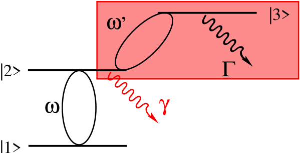
Figure 5: Effective description of the system of Fig. 4 in terms of only two levels: $\gamma=\omega^{\prime 2}/\Gamma$.

We now discuss a different regime, yielding a different Zeno picture. Rather than the situation (60), consider

$$\Gamma\ll\omega^{\prime}.$$ (67)

In this regime, the “control” of the evolution, performed by $\omega^{\prime}$, is made with no dissipation/measurement. Let us first discuss in which sense one gets a Zeno effect. Look at the idealized case $\Gamma=0$ (Fig. 6). The (Hermitian) Hamiltonian reads

$$H_{\mathrm{ideal}}=\frac{\omega}{2}(|1\rangle\langle 2|+|2\rangle\langle 1|)+\frac{\omega^{\prime}}{2}(|2\rangle\langle 3|+|3\rangle\langle 2|)=\frac{1}{2}\pmatrix{0&\omega&0\cr\omega&0&\omega^{\prime}\cr 0&\omega^{\prime}&0}:$$ (68)

we shall argue that level 3 plays here the effective role of measuring apparatus, although there is no bona fide measurement involved: as soon as the system is in $|2\rangle$ it undergoes Rabi oscillations to $|3\rangle$. We expect level $|3\rangle$ to perform better as a measuring apparatus when the strength $\omega^{\prime}$ of the coupling becomes larger.

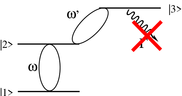
Figure 6: Three stable levels, no dissipation.

The survival probability in the initial state $|1\rangle$ reads

$$p_{1}(t)=\left|\langle 1|e^{-iH_{\mathrm{ideal}}t}|1\rangle\right|^{2}=\frac{1}{(\omega^{\prime 2}+\omega^{2})^{2}}\left[\omega^{\prime 2}+\omega^{2}\cos\left(\sqrt{\omega^{\prime 2}+\omega^{2}}t/2\right)\right]^{2}$$ (69)

and is shown in Fig. 7 for $\omega^{\prime}=1,3,9\,\omega$.

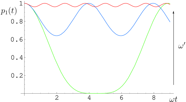
Figure 7: Survival probability for a continuous Rabi coupling with $\omega^{\prime}=\omega$ (green), $\omega^{\prime}=3\,\omega$ (blue), $\omega^{\prime}=9\,\omega$ (red).

We notice that for large $\omega^{\prime}$ the state of the system does not change much: as $\omega^{\prime}$ is increased, level $|3\rangle$ performs a better “observation” of the state of the system, hindering transitions from $|1\rangle$ to $|2\rangle$. This can be viewed as a QZE due to a continuous, Hermitian coupling to level $|3\rangle$. This is the situation displayed in Fig. 6.

Note that one can also interpret the above results as an experiment of electromagnetically induced transparency [43]. Indeed, the strong coupling $\omega^{\prime}$ between levels 2 and 3 splits state $|2\rangle$ into two dressed states $|\pm\rangle=(|2\rangle\pm|3\rangle)/\sqrt{2}$ of energy $\pm\omega^{\prime}$. For large values of $\omega^{\prime}$ these states run out of resonance and the system becomes transparent to the laser resonant with the transition $1\leftrightarrow 2$.

But what happens for small $\Gamma$? An expansion yields

$$p_{1}(t)\stackrel{{\scriptstyle\Gamma\;{\rm small}}}{{\simeq}}\frac{1}{(\omega^{\prime 2}+\omega^{2})^{2}}\left[\omega^{\prime 2}e^{-\Gamma\omega^{2}t/2(\omega^{2}+\omega^{\prime 2})}+\omega^{2}e^{-\Gamma\omega^{\prime 2}t/4(\omega^{2}+\omega^{\prime 2})}\cos(\sqrt{\omega^{\prime 2}+\omega^{2}}t/2)\right]^{2}.$$ (70)

We stress that this is a very accurate formula (technically, the expansion is uniform), essentially valid even for $\Gamma=O(\omega)$ or $\Gamma=O(\omega^{\prime})$ (or both!). The results are shown Fig. 8 for $\omega^{\prime}=1,3,9\,\omega$ and $\Gamma=0.2\,\omega$.

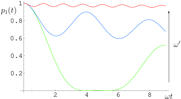
Figure 8: Survival probability for a continuous Rabi coupling with a small dissipation $\Gamma=0.2\,\omega$ on level #3. Like before, $\omega^{\prime}=\omega$ (green), $\omega^{\prime}=3\,\omega$ (blue), $\omega^{\prime}=9\,\omega$ (red).

In Figs. 7 and 8 we used arbitrary values of the parameters for the sake of illustration. It is remarkable how efficient the procedure turns out to be for more physical values of $\omega,\omega^{\prime},\Gamma$: one can get a quantitative idea by plotting (with care!) Eq. (70).

Clearly, in the very same regime (67), one can use a pulsed technique, as in Fig. 3. This is sometimes called “bang-bang.” In fact, it is nothing but pulsed Zeno.

9 Some comments on interpretation

Let us reinterpret the results of the previous section in the light of the theorem proved in Sec. 6. Reconsider Hamiltonian (68) (here $\omega^{\prime}$ plays the role of $K$ in Sec. 6)

$$H_{\mathrm{ideal}}=\frac{1}{2}\pmatrix{0&\omega&0\cr\omega&0&\omega^{\prime}\cr 0&\omega^{\prime}&0}=H+\omega^{\prime}H_{\mathrm{c}},$$ (71)

where

$$H=\frac{\omega}{2}(|1\rangle\langle 2|+|2\rangle\langle 1|)=\frac{\omega}{2}\pmatrix{0&1&0\cr 1&0&0\cr 0&0&0},$$ (72)

$$H_{\mathrm{c}}=\frac{1}{2}|2\rangle\langle 3|+|3\rangle\langle 2|=\frac{1}{2}\pmatrix{0&0&0\cr 0&0&1\cr 0&1&0}.$$ (73)

As $\omega^{\prime}$ is increased, the Hilbert space is split into three invariant subspaces (the eigenspaces of $H_{\mathrm{c}}$), ${\mathcal{H}}=\bigoplus{\mathcal{H}}_{P_{n}}$, with

$${\mathcal{H}}_{P_{0}}=\mathrm{span}\{|1\rangle\},\quad{\mathcal{H}}_{P_{1}}=\mathrm{span}\{|2\rangle+|3\rangle\},\quad{\mathcal{H}}_{P_{-1}}=\mathrm{span}\{|2\rangle-|3\rangle\},$$ (74)

corresponding to the projections

$$P_{0}=\pmatrix{1&0&0\cr 0&0&0\cr 0&0&0},\quad P_{1}=\frac{1}{2}\pmatrix{0&0&0\cr 0&1&1\cr 0&1&1},\quad P_{-1}=\frac{1}{2}\left(\begin{array}[]{rrr}0&0&0\\ 0&1&-1\\ 0&-1&1\end{array}\right),$$ (75)

with eigenvalues $\eta_{0}=0$ and $\eta_{\pm 1}=\pm 1$. The diagonal part of the system Hamiltonian $H$ vanishes, $H_{\mathrm{diag}}=\sum P_{n}HP_{n}=0$, and the Zeno evolution is governed by

$$H_{\mathrm{Z}}=\omega^{\prime}H_{\mathrm{c}}=\frac{1}{2}\pmatrix{0&0&0\cr 0&0&\omega^{\prime}\cr 0&\omega^{\prime}&0}.$$ (76)

Any transition between $|1\rangle$ and $|2\rangle$ is inhibited: a watched pot never boils.

10 A watched cook can freely watch a boiling pot

In the previous discussion we endeavored to make QZE on level 1. Essentially, a Rabi transition from $|1\rangle$ to $|2\rangle$ was inhibited by making use of different procedures. It would be interesting if one could hinder transitions out of a Zeno subspace, say a two-dimensional one, such as a qubit. Let us therefore modify the level scheme, in order to understand whether one can “protect” the evolution of a qubit. Let

$$\langle 0|=(1,0,0,0),\quad\langle 1|=(0,1,0,0),\quad\langle 2|=(0,0,1,0),\quad\langle 3|=(0,0,0,1)$$ (77)

and consider the four level Hamiltonian

$$H_{\mathrm{4lev}}=\pmatrix{0&\Omega&0&0\cr\Omega&0&\omega&0\cr 0&\omega&0&\omega^{\prime}\cr 0&0&\omega^{\prime}&0},$$ (78)

where states $|0\rangle$ and $|1\rangle$ undergo Rabi oscillations,

$$\Omega(|0\rangle\langle 1|+|1\rangle\langle 0|)=\pmatrix{0&\Omega&0&0\cr\Omega&0&0&0\cr 0&0&0&0\cr 0&0&0&0},$$ (79)

while state $|2\rangle$ “observes” $|1\rangle$

$$\omega(|1\rangle\langle 2|+|2\rangle\langle 1|)=\pmatrix{0&0&0&0\cr 0&0&\omega&0\cr 0&\omega&0&0\cr 0&0&0&0}$$ (80)

and state $|3\rangle$ “observes” $|2\rangle$

$$\omega^{\prime}(|2\rangle\langle 3|+|3\rangle\langle 2|)=\pmatrix{0&0&0&0\cr 0&0&0&0\cr 0&0&0&\omega^{\prime}\cr 0&0&\omega^{\prime}&0}.$$ (81)

For the sake of simplicity, we assumed no dissipation and redefined the Rabi frequencies in order to get rid of factors 2.

One can amuse oneself by deciding which “observation” is more effective [25, 44]. In the following, it is helpful to think of $|0\rangle$ and $|1\rangle$ as the states of a qubit ($\Omega$ being its dynamics), while $\omega$ is a caricature of a “decoherence” process and $\omega^{\prime}$ represents the “control” (whose objective is to suppress decoherence). See Fig. 9.

Figure 9: “Control” of the dynamics of a qubit and suppression of “decoherence.”

Let us consider the worst situation, where $\omega\gg\Omega$ and $\omega\gg\omega^{\prime}$. Then one easily shows that the total Hilbert space ${\mathcal{H}}$ splits into the three “Zeno” subspaces:

$${\mathcal{H}}_{0}=\mathrm{span}\{|0\rangle,|3\rangle\},\quad{\mathcal{H}}_{+}=\mathrm{span}\{|1\rangle+|2\rangle\},\quad{\mathcal{H}}_{-}=\mathrm{span}\{|1\rangle-|2\rangle\}$$ (82)

and the Zeno evolution is governed by

$$H_{\mathrm{4lev}}=\pmatrix{0&\Omega&0&0\cr\Omega&0&\omega&0\cr 0&\omega&0&\omega^{\prime}\cr 0&0&\omega^{\prime}&0}\stackrel{{\scriptstyle\omega\;{\rm large}}}{{\longrightarrow}}H^{(\omega)}_{\mathrm{Z}}=\pmatrix{0&0&0&0\cr 0&0&\omega&0\cr 0&\omega&0&0\cr 0&0&0&0}.$$ (83)

The Rabi oscillations between states $|0\rangle$ and $|1\rangle$ are hindered (as well as those between $|2\rangle$ and $|3\rangle$). The dynamics $\Omega$ of the qubit $\{|0\rangle,|1\rangle\}$ is destroyed by decoherence $\omega$. This is detrimental.

On the other hand, if $\omega^{\prime}\gg\omega$, and even if $\omega\gg\Omega$, the total Hilbert space splits into the three subspaces:

$${\mathcal{H}}^{\prime}_{0}=\mathrm{span}\{|0\rangle,|1\rangle\},\quad{\mathcal{H}}^{\prime}_{+}=\mathrm{span}\{|2\rangle+|3\rangle\},\quad{\mathcal{H}}^{\prime}_{-}=\mathrm{span}\{|2\rangle-|3\rangle\}$$ (84)

[notice the differences with (82)] and the Zeno Hamiltonian reads

$$H_{\mathrm{4lev}}=\pmatrix{0&\Omega&0&0\cr\Omega&0&\omega&0\cr 0&\omega&0&\omega^{\prime}\cr 0&0&\omega^{\prime}&0}\stackrel{{\scriptstyle\omega^{\prime}\;{\rm large}}}{{\longrightarrow}}H^{(\omega^{\prime})}_{\mathrm{Z}}=\pmatrix{0&\Omega&0&0\cr\Omega&0&0&0\cr 0&0&0&\omega^{\prime}\cr 0&0&\omega^{\prime}&0}.$$ (85)

The conclusions are interesting and beautiful: the Rabi oscillations between states $|0\rangle$ and $|1\rangle$ are fully preserved (even if and in spite of $\omega\gg\Omega$). This is the control of a qubit: its dynamics $\Omega$ is restored, even in presence of strong decoherence $\omega>$ (or even $\gg$) $\Omega$.

In conclusion, if $\omega^{\prime}\gg\omega,\Omega$, so that $\omega^{\prime-1}$ is the shortest timescale in the problem, a watched cook can freely watch a boiling pot. The suppression of the transition out of level 1 can be of great help in protecting the dynamics of the qubit $\{|0\rangle,|1\rangle\}$. Unlike the one-dimensional case, an experiment on the multidimensional QZE has a twofold objective: i) prevent probability leakage out of the Zeno subspace; ii) preserve the Zeno dynamics in the subspace. An experiment on the preservation of the Zeno dynamics of a multidimensional system (such as a qubit) has never been done.

11 Conclusions

We considered three physically equivalent formulations of the QZE and focused on the “continuous coupling” version, in order to analyze some simple examples involving two, three and four level systems. These examples are of interest in the light of possible applications. Among these, we considered the possibility of tailoring the interaction so as to obtain robust subspaces against decoherence, useful for applications in quantum computation. The experimental scheme proposed in Sec. 10 would enable one to control the dynamics of a qubit. It is remarkable that a problem like the quantum Zeno effect, that was considered academic until no more than 20 years ago, might lead in the next future to novel experiments and very practical applications, motivating the invention of techniques to counter decoherence and dissipation.

We would like to thank Wolfgang Ketterle for an interesting email exchange. This work is partially supported by the European Union through the Integrated Project EuroSQIP.

References

- [1] Misra B and Sudarshan E C G 1977 J. Math. Phys. 18 756
- [2] Gorini V, Kossakowski A and Sudarshan E C G 1976 J. Math. Phys. 17 821 \nonumLindblad G 1976 Comm. Math. Phys. 48 119
- [3] von Neumann J 1932 Die Mathematische Grundlagen der Quantenmechanik (Springer, Berlin). [English translation by E. T. Beyer 1955 Mathematical Foundation of Quantum Mechanics (Princeton University Press, Princeton)].
- [4] Beskow A and Nilsson J 1967 Arkiv für Fysik 34 561
- [5] Khalfin L A 1968 JETP Letters 8 65
- [6] Peres A 1980 Am. J. Phys. 48 931 \nonumKraus K 1981 Found. Phys. 11 547 \nonumSudbery A 1984 Ann. Phys. 157 512
- [7] Friedman C N 1972 Indiana Univ. Math. J. 21 1001 \nonumGustafson K and Misra B 1976 Lett. Math. Phys. 1 275 \nonumGustafson K 1983 Irreversibility questions in chemistry, quantum-counting, and time-delay, in Energy storage and redistribution in molecules, edited by Hinze J (Plenum, New York), and refs. [10,12] therein; \nonumGustafson K 2002 A Zeno story quant-ph/0203032
- [8] Exner P and Ichinose T 2005 Ann. H. Poincare 6 195 \nonumExner P, Ichinose T, Neidhardt H, Zagrebnov V 2007 57 67
- [9] Facchi P and Pascazio S 2008 J. Phys. A: Math. Theor. 41 493001
- [10] Cook, R J 1988 Phys. Scr. T 21 49
- [11] Itano W M, Heinzen D J, Bollinger J J and Wineland D J 1990 Phys. Rev. A 41 2295
- [12] Petrosky T, Tasaki S, and Prigogine I 1990 Phys. Lett. A 151 109 \nonumPetrosky T, Tasaki S, and Prigogine I 1991 Physica A 170 306 \nonumPeres A and Ron A 1990 Phys. Rev. A 42 5720 \nonumPascazio S, Namiki M, Badurek G and Rauch H 1993 Phys. Lett. A 179 155 \nonumAltenmüller T P andSchenzle A 1994 Phys. Rev. A 49 2016 \nonumCirac J I, Schenzle A and Zoller P 1994 Europhys. Lett. 27 123 \nonumPascazio S and Namiki M 1994 Phys. Rev. A 50, 4582 \nonumBerry M V 1995 Two-State Quantum Asymptotics, in Fundamental Problems in Quantum Theory, eds. \nonumGreenberger D M and Zeilinger A (Ann. N.Y. Acad. Sci. 755 303 \nonumBeige A and Hegerfeldt G 1996 Phys. Rev. A 53 53 \nonumLuis A and Peřina J 1996 Phys. Rev. Lett. 76, 4340 \nonumBeige A, Braun D, Tregenna B, and Knight P L 2000 Phys. Rev. Lett. 85 1762 \nonumAgarwal G S, Scully M O and Walther H 2001 Phys. Rev. Lett. 86 4271
- [13] Kwiat P, Weinfurter H, Herzog T, Zeilinger A, and Kasevich M 1995 Phys. Rev. Lett. 74 4763 \nonumNagels B, Hermans L J F and Chapovsky P L 1997 Phys. Rev. Lett. 79 3097 \nonumBalzer C, Huesmann R, Neuhauser W and Toschek P E 2000 Opt. Comm. 180 115 \nonumToschek P E and Wunderlich C 2001 Eur. Phys. J. D 14 387 \nonumWunderlich C, Balzer C, and Toschek P E 2001 Z. Naturforsch. 56a 160
- [14] Streed E W, Mun J, Boyd M, Campbell G K, Medley P, Ketterle W and Pritchard D E 2006 Phys. Rev. Lett. 97 260402
- [15] Bernu J, Deléglise S, Sayrin C, Kuhr S, Dotsenko I, Brune M, Raimond J M and Haroche S 2008 Phys. Rev. Lett. 101 180402
- [16] Jericha E, Schwab D E, Jäkel M R, Carlile C J, and Rauch H 200 Physica B 283, 414 \nonumRauch H 2001 Physica B 297 299
- [17] Wilkinson S R, Bharucha C F, Fischer M C, Madison K W, Morrow P R, Niu Q, Sundaram B and Raizen M G 1997 Nature 387 575
- [18] Fischer M C, Gutiérrez-Medina B and Raizen M G 2001 Phys. Rev. Lett. 87 040402
- [19] Lane A M 1983 Phys. Lett. A 99 359 \nonumSchieve W C, Horwitz L P and Levitan J 1989 Phys. Lett. A 136 264 \nonumKofman A G and Kurizki G 2000 Nature 405 546 \nonumElattari B and Gurvitz S A 2000 Phys. Rev. A 62 032102
- [20] Facchi P, Nakazato H and Pascazio S 2001 Phys. Rev. Lett. 86 2699
- [21] Kaulakys B and Gontis V 1997 Phys. Rev. A 56 1131 \nonumFacchi P, Pascazio S and Scardicchio A 1999 Phys. Rev. Lett. 83 61 \nonumFlores J C 1999 Phys. Rev. B 60 30) Flores J C 2000 Phys. Rev. B 62 R16291 \nonumGurvitz A 2000 Phys. Rev. Lett. 85 812 \nonumGong J and Brumer P 2001 Phys. Rev. Lett. 86 1741 \nonumLuis A 2001 J. Opt. B 3 238
- [22] Nakazato H, Namiki M and Pascazio S 1996 Int. J. Mod. Phys. B 10 247 \nonumHome D and Whitaker M A B 1997 Ann. Phys. 258 237
- [23] Facchi P and Pascazio S 2001 Progress in Optics, edited by E. Wolf (Elsevier, Amsterdam) 42 147
- [24] Facchi P, Gorini V, Marmo G, Pascazio S and Sudarshan E C G 2000 Phys. Lett. A 275 12 \nonumFacchi P, Pascazio S, Scardicchio A and Schulman L S 2002 Phys. Rev. A 65 012108
- [25] Facchi P and Pascazio S 2002 Phys. Rev. Lett. 89 080401
- [26] Simonius M 1978 Phys. Rev. Lett. 40 980 \nonumHarris R A and Stodolsky L 1978 Phys. Lett. B 78 313 \nonumHarris R A and Stodolsky L 1981 J. Chem. Phys. 74 2145 \nonumHarris R A and Stodolsky L 1982 Phys. Lett. B 116 464 \nonumCina J A and Harris R A 1995 Science 267 832 \nonumVenugopalan A and Ghosh R 1995 Phys. Lett. A 204 11 \nonumPlenio M P, Knight P L and Thompso R C 1996 Opt. Comm. 123 278 \nonumBerry M V and Klein S 1996 J. Mod. Opt. 43 165 \nonumPanov A D 1996 Ann. Phys. (NY) 249 1 \nonumMihokova E, Pascazio S and Schulman L S 1997 Phys. Rev. A 56 25 \nonumLuis A and Sánchez–Soto L L 1998 Phys. Rev. A 57 781 \nonumThun K and Peřina J 1998 Phys. Lett. A 249 363 \nonumSchulman L S 1998 Phys. Rev. A 57 1509 \nonumPanov A D 1999 Phys. Lett. A 260 441 \nonumŘeháček J, Peřina J, Facchi P, Pascazio S and Mišta L 2000 Phys. Rev. A 62 013804 \nonumFacchi P and Pascazio S 2000 Phys. Rev. A 62 023804 \nonumMilitello B, Messina A and Napoli A 2001 Phys. Lett. A 286 369 \nonumLuis A 2001 Phys. Rev. A 64 032104
- [27] Facchi P and Pascazio S 1998 Phys. Lett. A 241 139 \nonumFacchi P and Pascazio S 1999 Physica A 271 133 \nonumAntoniou I, Karpov E, Pronko G and Yarevsky E 2001 Phys. Rev. A 63 062110
- [28] Fermi E 1932 Rev. Mod. Phys. 4 87 \nonumFermi E 1950 Nuclear Physics (University of Chicago, Chicago) 136, 148 \nonumFermi E 1954 Notes on Quantum Mechanics. A Course Given at the University of Chicago in 1954, edited by Segré E (University of Chicago, Chicago) Lec. 23
- [29] Bernardini C, Maiani L and Testa M 1993 Phys. Rev. Lett. 71 2687 \nonumMaiani L and Testa M 1998 Ann. Phys. (NY) 263 353 \nonumJoichi I, Matsumoto Sh and Yoshimura M 1998 Phys. Rev. D 58 045004 \nonumAlvarez-Estrada R F and Sánchez-Gómez J L 1999 Phys. Lett. A 253 252 \nonumPanov A D 2000 Physica A 287 193
- [30] Lüders G 1951 Ann. Phys. (Leipzig) 8 322
- [31] Schwinger J 1959 Proc. Nat. Acad. Sc. 45 1552 \nonumSchwinger J 1991 Quantum kinematics and dynamics (Perseus Publishing, New York) p 26
- [32] Peres A 1998 Quantum Theory: Concepts and Methods (Kluwer Academic Publishers, Dordrecht)
- [33] Reed M and Simon B 1980 Functional Analysis I (Academic Press, San Diego) p 57
- [34] Facchi P, Lidar D A and Pascazio S 2004 Phys. Rev. A 69 032314
- [35] Messiah A 1961 Quantum mechanics (Interscience, New York) \nonumBorn M and Fock V 1928 Z. Phys. 51 165 \nonumKato T 1950 J. Phys. Soc. Jap. 5 435 \nonumAvron J E and Elgart A 1999 Comm. Math. Phys. 203 445 and references therein
- [36] Facchi P, Tasaki S, Pascazio S, Nakazato H, Tokuse A and Lidar D A 2005 Phys. Rev. A 71 022302
- [37] Wick G C , Wightman A S and Wigner E P 1952 Phys. Rev. 88 101 Wick G C , Wightman A S and Wigner E P 1970 Phys. Rev. D 1 3267
- [38] Jauch J M 1964 Helv. Phys. Acta 37 293
- [39] Berry M V Chaos and the semiclassical limit of quantum mechanics (is the moon there when somebody looks?), in Quantum Mechanics: Scientific perspectives on divine action (eds Robert John Russell, Philip Clayton, Kirk Wegter-McNelly and John Polkinghorne), Vatican Observatory CTNS publications p 41
- [40] Machida S and Namiki M 1980 Prog. Theor. Phys. 63 1457 \nonumMachida S and Namiki M 1980 Prog. Theor. Phys. 63 1833 \nonumAraki H 1962 Einführung in die Axiomatische Quantenfeldtheorie I, II (ETH-Lecture, ETH, Zurich) \nonumAraki H 1980 Prog. Theor. Phys. 64 719
- [41] Facchi P, Marmo G, Pascazio S, Scardicchio A and Sudarshan E C G 2004 J. Opt. B: Quantum Semicl. Opt. 6 S492
- [42] Cohen-Tannoudji C, Dupont-Roc J and Grynberg G 1998 Atom-Photon Interactions: Basic Processes and Applications (Wiley, New York)
- [43] Boller K J, Imamoglu A and Harris S E 1991 Phys. Rev. Lett. 66 2593
- [44] Militello B, Messina A and Napoli A 2001 Fortschr. Phys. 49 1041