The number of dimensional fundamental constants

Abstract

We revisit, qualify, and objectively resolve the seemingly controversial question about what is the number of dimensional fundamental constants in Nature. For this purpose, we only assume that all we can directly measure are space and time intervals, and that this is enough to evaluate any physical observable. We conclude that the number of dimensional fundamental constants is two. We emphasize that this is an objective result rather than a “philosophical opinion”, and we let it clear how it could be refuted in order to prove us wrong. Our conclusion coincides with Veneziano’s string-theoretical one but our arguments are not based on any particular theory. As a result, this implies that one of the three usually considered fundamental constants $G$, $c$ or $h$ can be eliminated and we show explicitly how this can be accomplished.

I Introduction

The problem of how many dimensional fundamental constants are in Nature has been subject of debate for a long time (see, e.g., Levy77 -Wilczek and references therein). In the beginning of the XX century, Planck stated that four dimensional constants were necessary and sufficient to describe all physical phenomena Planck . He named these constants $a$, $b$, $c$, and $f$, which turned out to be related to the modern constants $h$, $k$ and $G$ by $a=h/k$, $b=h$ and $f=G$. The symbol $c$ has been kept since then to represent the speed of light. Planck showed, furthermore, that these constants could be combined in order to get a “natural” system of three basic units: units of length $\ell_{P}=\sqrt{G\hbar/c^{3}}$, time $t_{P}=\sqrt{G\hbar/c^{5}}$, and mass $m_{P}=\sqrt{\hbar c/G}$. (Incidentally, their numerical values were close to the set of units previously suggested by Stoney in the context of electromagnetism Stoney even before the introduction of the Planck constant $h$.)

A closer analysis of the four Planck’s original dimensional constants has revealed that the combination $b/a$, namely $k$, turns out to be a conversion factor between temperature and energy units, leading to the well accepted conclusion that the Boltzmann constant has its origin in the historical fact that temperature was not early recognized as a manifestation of kinetic energy. Had temperature been defined, at early times, as twice the mean energy stored in each degree of freedom of a system in thermal equilibrium (whenever the equipartition energy principle is valid) and the Boltzmann constant would have the dimensionless value 1 (i.e., it would not have been introduced at all), in which case entropy would be also dimensionless.

The view that $G$, $c$ and $h$ would be the three fundamental constants of Nature is often expressed by means of the so called “cube of natural units” or “cube of theories” first introduced by Gamov, Ivanenko and Landau in the late twenties (see, e.g., Okun91 and references therein), where the three dimensional constants involved in the construction of the Planck basic units appear explicitly. The vertices of the cube would correspond to certain limiting regimes of the physical laws. For instance, the origin $(0,0,0)$ would correspond to non-relativistic mechanics, $(c^{-1},0,0)$ to Special Relativity, $(0,h,0)$ to non-relativistic quantum mechanics, $(c^{-1},0,G)$ to General Relativity and so on Okun91 (see left-hand side of Fig. 1).

Such a conception has been recently challenged. Veneziano has concluded through string-theoretical arguments that the number of dimensional fundamental constants would be two, while Duff has advocated for none at all Duffetal02 . This is quite unacceptable that this question is still controversial. The problem here does not concern the fact of not having an answer to some objective question but having different answers to the same question. Here we make a clear statement of the problem and present what we believe to be a final solution: the number of fundamental dimensional constants is two. We emphasize that our conclusion can be objectively refuted if it is shown that there exists some observable measured in laboratory that cannot be expressed in a basis of two independent observables as shown in Eq. (4). What we present here is, thus, an objective conclusion rather than a philosophical opinion.

II Space, time, and nothing else

Let us begin by clearly stating the points upon which our line of reasoning is based:

• Without going into the subtleties of precisely defining what a physical theory is, we only assume that any “good” physical theory should fulfill the following minimum criteria: (i) list the observables it deals with, (ii) prescribe how to measure these observables, and (iii) provide self-consistent relations among them (the “physical laws”);

• These relations are then tested against experimental data obtained through properly chosen processes, which we assume to take place in the spacetime; eventually, all we can directly measure are space and time intervals. In particular, this implies that one only needs two units to express all measurements.

The basic units of space and time, say $\sigma$ and $\tau$, respectively, can be chosen in a quite arbitrary way, and once this is done, any observable ${\cal O}_{i}$ can be expressed as

$${\cal O}_{i}=\Omega_{i}\,\tau^{{\alpha}_{i}}\sigma^{{\beta}_{i}},$$ (1)

with $\Omega_{i}$, $\alpha_{i}$, and $\beta_{i}$ being real (dimensionless) numbers, and $i$ belonging to some index set $\cal I$. For the sake of notation simplicity, the index $i$ gives information not only about the physical quantity being considered (energy, spin, …) but also about the state of the system (no matter how the theory chooses to describe it). As a result, $\Omega_{i}$, for given $i$, is indeed a real number instead of a real-valued function.

It is in order now to stress that one can select any pair $o_{1}$ and $o_{2}$ of independent observables to express all the other ones as follows. Since $o_{1},o_{2}\in\{{\cal O}_{i}\}_{i\in{\cal I}}$, let us cast them as

$$o_{1} = \Omega_{o_{1}}\tau^{a_{1}}\sigma^{b_{1}}\;,$$ (2)

$$o_{2} = \Omega_{o_{2}}\tau^{a_{2}}\sigma^{b_{2}}\;,$$ (3)

where by independent we mean that $(a_{1},b_{1})$ and $(a_{2},b_{2})$ form a basis of ${\mathbb{R}}^{2}$. Then, we can solve Eqs. (2) and (3) for $\tau$ and $\sigma$ and rewrite Eq. (1) associated with all other observables as

$${\cal O}_{i}={\widetilde{\Omega}}_{i}o_{1}^{\mu_{i}}o_{2}^{\nu_{i}}\;,$$ (4)

where ${\widetilde{\Omega}}_{i}$, $\mu_{i}$ and $\nu_{i}$ are clearly real numbers, namely,

$${\widetilde{\Omega}}_{i} = \Omega_{i}\;\Omega_{o_{1}}^{(-b_{2}\alpha_{i}+a_{2}\beta_{i})/W}\;\Omega_{o_{2}}^{(b_{1}\alpha_{i}-a_{1}\beta_{i})/W}\;,$$

$$\mu_{i} = (b_{2}\alpha_{i}-a_{2}\beta_{i})/W\;,$$

$$\nu_{i} = (-b_{1}\alpha_{i}+a_{1}\beta_{i})/W$$

and $W\equiv a_{1}b_{2}-b_{1}a_{2}$. The fact that $W\neq 0$ is guaranteed by our requirement that $o_{1}$ and $o_{2}$ be independent. Although the choice $\{o_{1},o_{2}\}\subset\{{\cal O}_{i}\}_{i\in{\cal I}}$ is arbitrary, there may be more convenient ways (possibly theory-dependent) of selecting this basic set. Indeed, the speed of light $c$ and the transition time $t_{Cs}$ between certain energy states of the Cesium atom, which are presently adopted to define the standard units of space and time Mohretal05 , could be naturally chosen to constitute the basic set.

At this point, let us clearly distinguish what we are saying from what we are not saying. Our conclusion that all the observables ${\cal O}_{i}$ can be expressed in terms of only two basic dimensional observables does not imply the existence of some “final” theory able to predict all dimensionless real numbers ${\widetilde{\Omega}}_{i}$ appearing in Eq. (4) (no matter how desirable it may be). For instance, in the Standard Model the total number of dimensional and dimensionless parameters which should be provided as input in order to predict all the other observables is much larger than two. However, one can choose any pair of independent dimensional constants from this set and express all the other ones (and, consequently, all observables) in terms of this pair.

III Measuring mass with clocks and rulers

A question which can be raised is how observables which are usually written not only in terms of space and time units, e.g. mass, fit into this scheme. We exhibit next two protocols where the mass unit $M$ (g, pounds, …) is solely expressed in terms of units of space and time. For the sake of simplicity, in both protocols we start assuming the CGS system, where all observable quantities ${\cal D}_{i}$ are expressed in terms of units of space $L$ (cm), time $T$ (s), and mass $M$ (g):

$${\cal D}_{i}=\Delta_{i}\;T^{{\alpha}_{i}}L^{{\beta}_{i}}M^{{\gamma}_{i}}\;,$$ (5)

where $\Delta_{i}$, $\alpha_{i}$, $\beta_{i}$, and $\gamma_{i}$ are real numbers.

• $G$ protocol: Multiply Eq. (5) by $G^{\gamma_{i}}$, where $G$ is the Newton’s constant, and identify ${\cal D}_{i}G^{\gamma_{i}}$ as the observable ${\cal O}_{i}^{(G)}$ which appears in Eq. (1) (and fulfills our conditions 1.–2.). [Here the superscript $(G)$ is introduced only to indicate the protocol used to cast the observable in the form given by Eq. (1).] By using the $G$ protocol in all observables involving the $M$ unit and rewriting the physical laws in terms of ${\cal O}_{i}^{(G)}$ rather than ${\cal D}_{i}$, we end up (i) vanishing the unit $M$ (g) from the observables, (ii) vanishing the constant $G$ from all physical laws, and (iii) with masses being measured in units of ${\rm cm}^{3}/{\rm s}^{2}$. For instance, by applying the $G$ protocol to the original Newton’s gravitational law $g=-Gm/d^{2}$, we get

  $$g=-\,{m^{(G)}}/{d^{2}}\;,$$ (6)

  where the units of $m^{(G)}\equiv m\,G$ is $L^{3}/T^{2}$. In this sense, $G$ plays the role of a conversion factor (from ${\rm cm}^{3}/{\rm s}^{2}$ to g) as much as does the Boltzmann constant $k$ (from erg to Kelvin). Indeed, $G$ could have never been introduced once the mass unit were properly defined (see Sec. 11 of Ref. Buckingham14 and Ref. Okunetal02 ). We see from Eq. (6) that this procedure of eliminating the unit of mass $M$ leads $m^{(G)}$ to be directly interpreted as (and not only related to) active gravitational mass, and that it can be obtained simply through space and time measurements by determining the acceleration $g$ induced on test particles lying at a distance $d$. Moreover, we note for further purposes that the $G$ protocol applied to (the observable) Planck’s constant $h$ leads to

  $$h^{(G)}\equiv h\,G\;,$$ (7)

  whose dimension is $L^{5}/T^{3}$.

• $h$ protocol: Divide Eq. (5) by $h^{\gamma_{i}}$, where $h$ is Planck’s constant, and identify ${\cal D}_{i}/h^{\gamma_{i}}$ as the observable ${\cal O}_{i}^{(h)}$ which satisfies Eq. (1). By rewriting the physical laws in terms of ${\cal O}_{i}^{(h)}$ rather than ${\cal D}_{i}$, we end up (i) vanishing the unit $M$ (g) from the observables as before, (ii) vanishing the constant $h$ from all physical laws, and (iii) with masses being measured in units of ${\rm s}/{\rm cm}^{2}$. For instance, by applying the $h$ protocol to the original Compton scattering formula $\Delta\lambda=[h/(mc)](1-\cos\theta)$, we get

  $$\Delta\lambda=[m^{(h)}c]^{-1}(1-\cos\theta)\;,$$ (8)

  where the unit of $m^{(h)}\equiv m/h$ is $T/L^{2}$. In this sense, $h$ plays the role of a conversion factor (from ${\rm s}/{\rm cm}^{2}$ to g). In this protocol the inverse of the Compton length can be seen to be naturally associated with inertia of elementary particles through the Compton effect. Here $m^{(h)}c$ (and therefore $m^{(h)}$) can be directly measured using clocks and rulers by determining the wavelength change $\Delta\lambda$ of a photon scattered by an angle $\theta$. We note that the $h$ protocol applied to Newton’s constant $G$ leads to

  $$G^{(h)}\equiv Gh\;;$$ (9)

  Note that $G^{(h)}=h^{(G)}$. (A sort of implementation of the $h$ protocol can be found in Refs. Hoyle -Wignall .)

Some physical observables of interest in the different protocols are shown in Table 1.

	$G$ protocol	$h$ protocol
$G$	$G^{(G)}=1$	$G^{(h)}=4.42\times 10^{-34}\;{\rm cm}^{5}/{\rm s}^{3}$
$h$	$h^{(G)}=4.42\times 10^{-34}\;{\rm cm}^{5}/{\rm s}^{3}$	$h^{(h)}=1$
$m_{e}$	$m_{e}^{(G)}=6.08\times 10^{-35}\;{\rm cm}^{3}/{\rm s}^{2}$	$m_{e}^{(h)}=1.38\times 10^{-1}\;{\rm s}/{\rm cm}^{2}$
$e$	$e^{(G)}=1.24\times 10^{-13}\;{\rm cm}^{3}/{\rm s}^{2}$	$e^{(h)}=0.59\times 10^{4}\;{\rm cm}^{1/2}/{\rm s}^{1/2}$

Table 1: The values of $G$, $h$, and the electron mass and charge are presented in the $G$ and $h$ protocols. It is interesting to note that $h^{(G)}=G^{(h)}$.

Rewriting the physical laws in terms of Eq. (4) rather than Eq. (5) does not change any of their predictions. Nevertheless, it can shed new light on some conceptual issues. Next, we discuss and resolve in this context the much-debated question about what is the number of dimensional fundamental constants in Nature.

IV Physical Insights

In the previous section we presented two protocols in which mass can be determined through space and time measurements alone. In order to do so, each one of those protocols made use of a specific law relating mass with space and time intervals. However, since we claim that our main conclusion (regarding the number of dimensional fundamental constants) is general and theory-independent, one might wonder “what if Nature did not comply with any such a law?” For the sake of concreteness, let us imagine that Newtonian mechanics in the absence of gravity were all that there was to the laws of Nature. How would our arguments apply in this case?

Firstly, it is important (though obvious) to point out that Nature would look completely different. In that case, (inertial) mass would no longer be determined in terms of space and time measurements and a standard of mass, let us say the kilogram, might be introduced. Any mass would then be determined as some multiple of this standard mass through, e.g., colision experiments (recall that gravity is not available). Our point, however, is that in this case mass is no longer an observable as defined in Eq. (1), and, therefore, the laws of Nature can be rewritten in such a way to completely avoid the appearance of mass. This is certainly possible according to our definition of “physical law” given in point 1. of Sec. II, although they may look more complicated and appear in a larger number in this rewritten form. Once that is done, we are left again with only space and time units.

For those (like some of the authors) who would rather take the philosophical stand that even in the context above (Newtonian mechanics with no gravity) mass should be considered as “observable” (in some extended sense) due to the simplification it brings to the form of the physical laws, we point out that the need for an independent standard in this case reflects the fact that mass would be determined only up to a multiplicative constant: no mass scale would be privileged (Nature would be completely different indeed). Therefore, this new standard (introduced only to comply with someone’s prejudice) would not appear in any “objective fundamental constant” (i.e., those which determine “fundamental scales”, as most people seem to interpret what a fundamental constant is). Interestingly enough, in this same context a similar argument can be applied to space and time units to show that Newtonian mechanics in the absence of gravity has no “objective fundamental constants” at all (no fundamental space or time scales). The fact that we experience space and time as distinct entities and that Nature does not present itself invariant under rescale of these quantities seem to indicate that there should indeed exist fundamental scales of space and time. It is a remarkable fact that we have already reached an understanding of the physical laws from which these scales can be read out.

Since Nature does provide ways of measuring mass in terms of space and time intervals (the $G$ and $h$ protocols), the main relevance of the discussion above lies in the fact that it can be applied to any “observable” (in the extended sense) which may appear in some (still unknown) physical law: the “observable” is either determined in terms of space and time measurements (a true observable) or it cannot appear in determining fundamental constants which set scales in Nature.

Up to this point, our discussion was quite general and our conclusions followed directly from assumptions 1.-2. of Sec. II. Here, we raise accordingly some speculative physical considerations, which may be of some relevance. For this purpose, we choose the protocol $G$.

Firstly, we note that the protocol $G$ frees classical mechanics from its only (so called) “fundamental parameter”, namely, Newton’s gravitational constant. This is very convenient since the value of $G$ (like the value of $k$) does not determine any scale for new physics, in contrast to, e.g., $c$ and $h$, which fix a velocity and an angular momentum scale, respectively, where relativistic and quantum mechanical effects become important. In the $G$ protocol it becomes clear that classical mechanics does not have any prefered basis $\{o_{1},o_{2}\}$ of independent observables (see the origin of the plane of theories in Fig. 1). Newton’s gravitational and second laws are written in this context as

$$F_{g}^{(G)}=m^{(G)}M^{(G)}/r^{2},\;\;\;{\rm and}\;\;\;F^{(G)}_{I}=m^{(G)}a,$$ (10)

respectively. By comparing Eq. (10) with the Coulomb law $F_{C}^{(G)}=q^{(G)}Q^{(G)}/r^{2}$ we see that (gravitational) mass and electric charge have the same status as coupling constants of the respective interactions, as they should. The fact that gravitational mass happens to give also a measure of inertia is a separate, more profound issue, only partially addressed by General Relativity .

The actual bias driven by our present theories suggests that a natural basis of independent observables would be $\{c,h^{(G)}\}$. The vertices $(c^{-1}=0,h^{(G)})$ and $(c^{-1},h^{(G)}=0)$ in the plane of theories (see Fig. 1) represent non-relativistic and classical physics, respectively. It is interesting to note that in this scenario what we usually denominate (a) quantum gravity (whatever it is) and (b) quantum field theory would dwell at the same vertex $(c^{-1},h^{(G)})$ of Fig. 1. This would be reflecting the expected feature that a complete theory (which we call here quantum relativity) describing consistently all interactions (including gravity) should contain (a) and (b). We note that quantum relativity effects can appear at quite low energies. The Hawking temperature

$$(kT_{H})^{(G)}=\frac{\hbar^{(G)}c^{3}}{8\pi M^{(G)}}$$

associated with the evaporation of (static) black holes with mass $M^{(G)}$ is a good example of it. If $c$ were substantially larger, $(kT_{H})^{(G)}$ would be able to be trivially tested in stellar-size black holes. A distinct point that becomes obvious in the context of the $G$ protocol is that an electron has much more electric than “gravitational” charge: $e^{(G)}=2\times 10^{21}m_{e}^{(G)}$. On the other hand General Relativity tells us that if a (classical) black hole is given more charge than mass it becomes a naked singularity. Naked singularities are expected to be understood only in the context of quantum gravity. If quantum gravity and quantum field theory are both different aspects of a single quantum relativity theory, it is possible that naked singularities and elementary particles be understood by the same token. This is not odd if one notices that the Planck scale for the angular momentum is precisely given by $h^{(G)}$.

V Conclusions

As a result of our conclusion that all observables can be expressed as in Eq. (4), any physical theory fulfilling conditions 1.–2. will not require more than a pair of independent dimensional constants to be expressed. This pair of observables is what one usually denominates fundamental (dimensional) constants. Both protocols that we have presented favor $c$ and $h^{(G)}$ ($=G^{(h)}$) to constitute this pair but other protocols could be easily devised (e.g., replacing $h$ by $e^{2}$ in the $h$ protocol). From a theory-independent perspective, no protocol can be privileged. However, some distinction can be made if we allow for biases coming from the present theories. In this sense, both the $G$ and $h$ protocols exhibit the nice feature of selecting as fundamental constants $c$ and $h^{(G)}$, which define the regimes where relativistic and quantum effects become important, respectively. Our conclusion that two ($c$, $h^{(G)}$) rather than three ($c$, $h$, $G$) dimensional fundamental constants suffice can be nicely represented as in Fig. 1 by the squashing of the cube of theories. Clearly, other choices of fundamental constants may become more convenient depending on future developments of our theories. Eventually, for a full quantum gravity (or “quantum relativity”) theory, the following pair may be more convenient: $t_{P}=(h^{(G)}/c^{5})^{1/2}$ and $\ell_{P}=(h^{(G)}/c^{3})^{1/2}$ (see Fig. 2).

In order to avoid any misunderstanding, let us clarify one point which might cause some confusion. After adopting the $G$ (or $h$) protocol to eliminate the mass unit $M$ from all quantities in Eq. (5), one could easily envisage an extra protocol to carry out the elimination of one of the remaining units $T$ or $L$, e.g., a “$c$ protocol”, in which case all quantities would be expressed accordingly as multiples of some power of $L$ or $T$ alone. In fact, one could proceed even further and use the other fundamental constant $h^{(G)}$ (after properly redefined through the hypothetical $c$ protocol) and vanish the sole unit left. In this case, all quantities would be dimensionless numbers. Although this is true, it does not imply that the number of dimensional fundamental constants would be one or zero explanation . We must recall that our line of reasoning is based on points 1.–2. of Sec. II, and not on the existence of some protocol to lower the number of units in physical equations. The latter only eliminates unnecessary structures once the number of dimensional fundamental constants is established. After all, our conclusion that the number of dimensional fundamental constants is two comes from the following facts: (i) space and time are distinct entities (a fact which should be accounted for in any “complete theory”) and (ii) combined measurements of space and time suffice to characterize any physical system. Points (i) and (ii) above set the lower and upper bounds, respectively, for the number of dimensional fundamental constants to be two. Our conclusions are in agreement with Veneziano (see Ref. Duffetal02 ) but our arguments are model independent.

We emphasize once again that our conclusion above can be objectively refuted if it is shown that there exists some observable measured in laboratory that cannot be expressed in a basis of two independent observables as shown in Eq. (4). This is, thus, an objective conclusion rather than a philosophical opinion. A number of valuable papers reformulating physical theories in a more transparent or elegant way can be found in the literature. We hope that our paper is appreciated in the same lines with the difference that it deals with the whole set of physical theories.

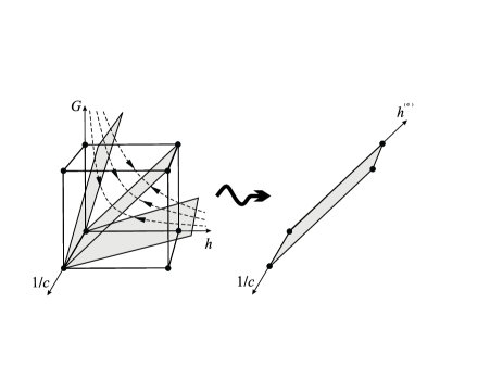
Figure 1: The cube of theories is shown in the left-hand side. The origin $(0,0,0)$ corresponds to non-relativistic mechanics, $(c^{-1},0,0)$ to Special Relativity, $(0,h,0)$ to non-relativistic Quantum Mechanics, $(0,0,G)$ to Newtonian gravity, $(c^{-1},0,G)$ to General Relativity, $(0,h,G)$ to “non-relativistic Quantum Gravity”, $(c^{-1},h,0)$ to usual Quantum Field Theory, and $(c^{-1},h,G)$ to “Quantum Gravity”. After using the $G$ or $h$ protocols we end up with $h^{(G)}(=G^{(h)})$ rather than with $G$ and $h$. This leads the cube of theories to be squashed into a “plane of theories” as shown in the right-hand side of the figure. In the light of the $G$ protocol, for instance, the origin $(0,0)$ corresponds to non-relativistic mechanics, $(c^{-1},0)$ to Relativity, $(0,h^{(G)})$ to (non-relativistic) Quantum Mechanics and $(c^{-1},h^{(G)})$ to “relativistic Quantum Mechanics” (which includes Quantum Field Theory and Quantum Gravity).

Figure 2: The plane of theories can be covered by the lines of constant $h^{(G)}$ and $c^{-1}$ (horizontal and vertical dashed lines, respectively) or, equivalently, by the lines of constant $\ell_{P}$ and $t_{P}$.

- (1) J. M. Lévy-Leblond, Riv. Nuovo Cimento 7, 187 (1977).
- (2) S. Weinberg, Phil. Trans. R. Soc. Lond. A 310, 249 (1983).
- (3) F. Wilczek, Physics Today 58(10), 12 (2005); ibid 59(1), 10 (2006); ibid 59(5), 10 (2006).
- (4) M. Planck, S.-B. Preuss Akad. Wiss. 440 (1899); Ann. Phys. 1, 69 (1900).
- (5) G. J. Stoney, Philos. Mag. 11, 381 (1881).
- (6) L. B. Okun, Sov. Phys. Usp. 34, 818 (1991); Lect. Notes Phys. 648, 57 (2004) [physics/0310069].
- (7) M. J. Duff, L. B. Okun, and G. Veneziano, J. High Energy Phys. 03, 023 (2002).
- (8) P. J. Mohr and B. N. Taylor, Rev. Mod. Phys. 77, 1 (2005). S. G. Karshenboim, Can. J. Phys. 83, 767 (2005) [physics/0506173].
- (9) E. Buckingham, Phys. Rev. 4, 345 (1914).
- (10) G. Fiorentini, L. B. Okun, and M. Vysotskii, JETP Lett. 76, 485 (2002).
- (11) F. Hoyle and J. V. Narlikar, Action at a Distance in Physics and Cosmology, (Freeman and Company, San Francisco, 1974).
- (12) J. W. G. Wignall, Phys. Rev. Lett. 68, 5 (1992); Int. J. Mod. Phys. A15, 875 (2000).
- (13) Note that a physical law can always be rewritten in terms of dimensionless numbers as by using our Eq. (4). Eventually, this is the trivial fact which leads Duff to conclude that the number of dimensional fundamental constants would be zero. Although indeed implies that we do not need dimensional constants to express a physical law, we still need two independent dimensional standards [see in Eq. (4)] in order to measure and then test the physical law.