e-mail muljarov@gpi.ru

XXXX

Exciton dephasing in quantum dots: Coupling to LO phonons via excited states

Abstract

We have found a novel mechanism of spectral broadening and dephasing in quantum dots (QDs) due to the coupling to longitudinal-optical (LO) phonons. In theory, this mechanism comes into play only if the complete manifold of exciton levels (including those in the wetting-layer continuum) is taken into account. We demonstrate this nontrivial dephasing in different types of QDs, using the exactly solvable quadratic coupling model, here generalized to an arbitrary number of excitonic states.

While acoustic phonons are known to produce a spectral broadening of the exciton zero phonon line (ZPL) in QD spectra, it is widely believed that the coupling to bulk dispersionless LO phonons forms everlasting mixed states (exciton polarons) showing no line broadening [1, 2]. This is indeed true if the model is restricted to a limited number of exciton states. However, including a sufficiently large number of states results in spectral broadening and dephasing. We have recently demonstrated [3] this nontrivial and quite unexpected mechanism of dephasing using the exactly solvable quadratic coupling model earlier developed for acoustic phonons [4]. This new mechanism is in clear contrast with the acoustic phonon-induced dephasing as the latter provides a finite ZPL width due to the phonon-mediated coupling already to the next exciton level.

In this contribution, we derive the quadratic coupling model for a single level (exciton ground state) from the standard linear coupling between exciton levels in a QD and bulk LO phonons. Exciton excited states then contribute effectively through virtual transitions. We have generalized the exact solution of the model with two levels [5] to an arbitrary number of states [3]. Here we show explicitly a diagonalization of the quadratic Hamiltonian and then calculate the dephasing in different types of QDs.

We derive the model of quadratic coupling to LO phonons from the standard Hamiltonian with a linear exciton-phonon coupling:

$$H = \omega_{0}\sum_{\bf q}\left(a^{\dagger}_{\bf q}a_{\bf q}+\frac{1}{2}\right)+\sum_{n}E_{n}|n\rangle\langle n|$$ (1)

$$+\sum_{nm}|n\rangle\langle m|\sum_{\bf q}M_{nm}({\bf q})(a_{\bf q}+a^{\dagger}_{-\bf q})\,,$$

where $\omega_{0}$ is the dispersionless LO phonon frequency, $E_{n}$ is the bare transition energy of a single-exciton state $|n\rangle$ in a QD, $M_{nm}({\bf q})\propto q^{-1}\langle n|e^{i{\bf qr}_{e}}-e^{i{\bf qr}_{h}}|m\rangle$ are matrix elements of the linear exciton-phonon Fröhlich interaction, and $\hbar=1$. This problem has been solved exactly in case of a few exciton levels [2], but generally it is not solvable for an arbitrary number of levels because of the level-nondiagonal coupling which is, at the same time, of key importance for the dephasing. To preserve this coupling, on the one hand, and to bring the problem to an exactly solvable form, on the other, we make the following unitary transformation

$$H^{\prime}=e^{S}He^{-S}=H+[S,H]+[S,[S,H]]/2+\dots\,,$$ (2)

where the transformation operator $S$ has the form:

$$S = \sum_{n\neq m}|n\rangle\langle m|\sum_{\bf q}M_{nm}({\bf q})$$ (3)

$$\times\left(\frac{a_{\bf q}}{E_{n}-E_{m}-\omega_{0}}+\frac{a^{\dagger}_{-\bf q}}{E_{n}-E_{m}+\omega_{0}}\right)\,.$$

This transformation eliminated nondiagonal terms in first order [4], by mapping them into diagonal ones which are however quadratic in phonon operators. Higher powers of $M_{nm}({\bf q})$ are also generated in the transformed Hamiltonian. However, far from resonance where the quadratic coupling model is valid, they lead only to small quantitative corrections and thus can be safely neglected.

For the ground exciton state ($n=1$) the resulting quadratic Hamiltonian takes the form:

$$H_{1} = E^{\prime}_{1}+\omega_{0}\sum_{\bf q}\left(a^{\dagger}_{\bf q}a_{\bf q}+\frac{1}{2}\right)$$ (4)

$$+\sum_{\bf q}M_{11}({\bf q})\,(a_{\bf q}+a_{\bf-q}^{\dagger})$$

$$-\frac{1}{2}\sum_{\bf p\,q}Q({\bf p},{\bf q})\,(a_{\bf p}+a_{\bf-p}^{\dagger})(a_{\bf q}+a_{\bf-q}^{\dagger})\,,$$

where

$$E^{\prime}_{1}=E_{1}+\sum_{n\neq 1}\sum_{\bf q}\frac{|M_{1n}({\bf q})|^{2}\omega_{0}}{[(E_{n}-E_{1})^{2}-\omega_{0}^{2}]}$$

is a renormalized (polaron shifted) energy of the exciton ground state, and

$$Q({\bf p,q}) = 2\sum_{n\neq 1}\frac{E_{n}-E_{1}}{(E_{n}-E_{1})^{2}-\omega_{0}^{2}}\,M_{1n}({\bf p})M_{n1}({\bf q})$$ (5)

$$\equiv \sum_{n\neq 1}F_{n}({\bf p})F_{n}({\bf q})$$

is the kernel of the quadratic coupling, here expressed in terms of new functions $F_{n}({\bf q})$. Note that the Hamiltonian Eq.(4) contains also the state-diagonal linear coupling $M_{11}$.

The absorption spectrum is calculated as a Fourier transform of the linear response on a delta-pulse excitation,

$$P(t)=\theta(t)\langle e^{iH_{0}t}e^{-iH_{1}t}\rangle,$$ (6)

where a finite-temperature expectation value is taken over the unperturbed phonon system

$$H_{0}=\omega_{0}\sum_{\bf q}\left(a^{\dagger}_{\bf q}a_{\bf q}+\frac{1}{2}\right).$$

To do so we follow the method of Ref. [2] and diagonalize $H_{1}$ directly in a few successive steps.

First of all, we make a shift transformation:

$$b_{\bf q}=a_{\bf q}+f_{\bf q}$$ (7)

($f_{\bf q}$ will be given later). This is only to eliminate the linear coupling $M_{11}$, all other terms in Eq.(4) remaining the same, except for a new renormalization of the transition energy to $\widetilde{E}_{1}=E^{\prime}_{1}+E_{\rm pol}^{(2)}$ with an additional polaron shift $E_{\rm pol}^{(2)}=-\sum_{\bf q}M_{11}({\bf q})f_{\bf q}$. The next step is a rotation of the phonon basis, in order to make the quadratic coupling diagonal. To do this we diagonalize the Hermitian matrix ($E_{n}-E_{1}>\omega_{0}$ is assumed for simplicity):

$$A_{nm}\equiv\sum_{\bf q}F_{n}(-{\bf q})F_{m}({\bf q})=\sum_{\nu}\Lambda_{\nu}\,X_{\nu n}X^{\ast}_{\nu m}$$ (8)

and introduce new phonon operators:

$$B_{\nu}=\sum_{\bf q}C_{\nu}({\bf q})\,b_{\bf q}$$ (9)

with

$$C_{\nu}({\bf q})=\frac{1}{\sqrt{\Lambda_{\nu}}}\sum_{n}F_{n}({\bf q})X_{\nu n}$$ (10)

making the transformation orthogonal,

$$\sum_{\bf q}C^{\ast}_{\nu}({\bf q})C_{\mu}({\bf q})=\delta_{\nu\mu}\,.$$

Our calculation of the optical polarization $P(t)$ also needs to adapt the unshifted operators $a_{\bf q}$ to the form of Eq.(9) by making a similar transformation,

$$A_{\nu}=\sum_{\bf q}C_{\nu}({\bf q})a_{\bf q}\,,$$ (11)

which preserves diagonality of the unperturbed Hamiltonian due to negligible LO phonon dispersion:

$$H_{0}=\omega_{0}\sum_{\nu}\left(A^{\dagger}_{\nu}A_{\nu}+\frac{1}{2}\right).$$ (12)

For the perturbed Hamiltonian $H_{1}$, the diagonalization procedure is finalized as follows

$$H_{1}-\widetilde{E}_{1} = \sum_{\nu}\left[\omega_{0}\left(B^{\dagger}_{\nu}B_{\nu}+\frac{1}{2}\right)-\frac{1}{2}\Lambda_{\nu}(B_{\nu}+B^{\dagger}_{\nu})^{2}\right]$$ (13)

$$= \sum_{\nu}\Omega_{\nu}\left(\widetilde{A}^{\dagger}_{\nu}\widetilde{A}_{\nu}+\frac{1}{2}\right)\,,$$

where we have switched to another Bose operators

$$\widetilde{A}_{\nu}=\alpha^{+}_{\nu}B_{\nu}+\alpha^{-}_{\nu}B^{\dagger}_{\nu}=\alpha_{\nu}^{+}A_{\nu}+\alpha^{-}_{\nu}A^{\dagger}_{\nu}+\psi_{\nu}$$ (14)

with

$$\Omega_{\nu}=\sqrt{\omega_{0}^{2}-2\omega_{0}\Lambda_{\nu}}\,,$$ (15)

$$\alpha^{\pm}_{\nu}=\frac{\Omega_{\nu}\pm\omega_{0}}{\sqrt{\Omega_{\nu}\omega_{0}}}\,,$$

$$\psi_{\nu}=\alpha^{+}_{\nu}\phi_{\nu}+\alpha^{-}_{\nu}\phi^{\ast}_{\nu}\,,$$

$$\phi_{\nu}=\sum_{\bf q}C_{\nu}({\bf q})f_{\bf q}=\frac{1}{\omega_{0}-2\Lambda_{\nu}}\sum_{\bf q}C_{\nu}({\bf q})M_{11}({\bf-q})\,.$$

Now the linear polarization obviously becomes a product of contributions from independent phonon subsystems (labelled by the index $\nu$):

$$P(t) = \theta(t)e^{-i\widetilde{E}_{1}t}$$

$$\times \prod_{\nu}\sum_{kl}\gamma\exp\{-\beta\epsilon_{k}^{\nu}-i(\varepsilon_{l}^{\nu}-\epsilon_{k}^{\nu})t\}\,|\langle k;\nu|l;\nu\!\!>\!\!|^{2},$$

where $\varepsilon_{l}^{\nu}=(l+1/2)\Omega_{\nu}$ and $\epsilon_{k}^{\nu}=(k+1/2)\omega_{0}$ are, respectively, eigenenergies of the partial Hamiltonians $H_{1\nu}$ and $H_{0\nu}$:

$$H_{1}-\widetilde{E}_{1} = \sum_{\nu}H_{1\nu}\,,\ \ \ \ \ \ H_{1\nu}|l;\nu\!\!>=\varepsilon_{l}^{\nu}|l;\nu\!\!>,$$ (17)

$$H_{0} = \sum_{\nu}H_{0\nu}\,,\ \ \ \ \ \ H_{0\nu}|k;\nu\rangle=\epsilon_{k}^{\nu}|k;\nu\rangle,$$ (18)

$\beta=1/k_{B}T$, and $\gamma=2\cosh(\beta\omega_{0}/2)$. The projections $z^{l}_{k}(\nu)=\langle k;\nu|l;\nu\!\!>$ of the perturbed phonon states ($\widetilde{A}_{\nu}$) into the bare ones ($A_{\nu}$) are calculated recursively (below the index $\nu$ is omitted for simplicity; $k,l\geq 0$):

$$\sqrt{l+1}\,z_{k}^{l+1} = \alpha^{+}\sqrt{k}\,z_{k-1}^{l}+\alpha^{-}\sqrt{k+1}\,z_{k+1}^{l}+\psi^{\ast}z_{k}^{l}\,,$$

$$\sqrt{l}\,z_{k}^{l-1} = \alpha^{+}\sqrt{k+1}\,z_{k+1}^{l}+\alpha^{-}\sqrt{k}\,z_{k-1}^{l}+\psi z_{k}^{l}\,,$$

where the second equation can be used to determine the start values for the recursion ($l=0$), together with a normalization condition $\sum_{k=0}^{\infty}|z_{k}^{0}|^{2}=1$.

In case of two levels (only one excited state $n=2$ is taken into account), the matrix $A_{nm}$ becomes a scalar [see Eq.(8)] and thus only one phonon mode is renormalized. This phonon mode is bound to the QD and has a new frequency $\Omega$ given by Eq.(15). Due to the LO phonon degeneracy, all the other phonon modes are decoupled and thus do not contribute to the spectrum. In fact, the remaining phonon modes can be always orthogonalized (with respect to the bound modes) without change of their frequency. According to Eq.(LABEL:P), the spectrum represents a set of discrete lines with a fine structure splitting given by the difference between $\omega_{0}$ and $\Omega$, see Fig.1 (a). Increasing the number of exciton levels participating in the coupling, the number of bound phonon modes (having renormalized frequencies, Eq.(15), different from $\omega_{0}$) also increases and thus delta lines in the spectrum become more dense, see Fig.1 (b) and (c). Finally, if we include all exciton levels, these lines merge and produce a continuous spectral broadening, Fig.1 (d).

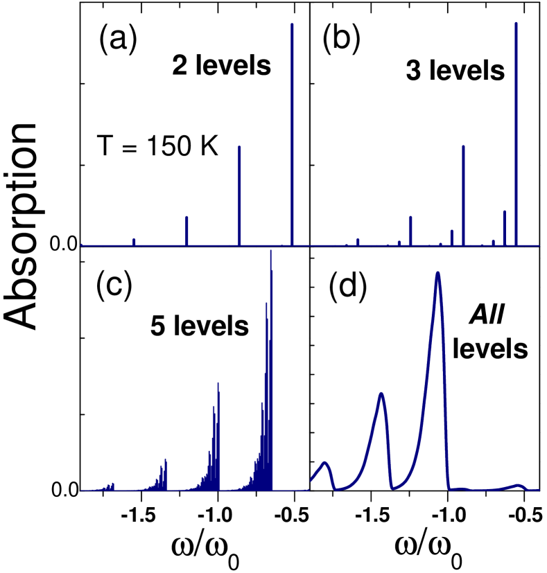
Figure 1: Calculated absorption spectra of the ground exciton state in a CdSe QD in the model of infinite harmonic potentials with the distance of 80 meV (35 meV) between electron (hole) levels coupled to LO phonons ($\omega_{0}=24$ meV).

Figure 2: Black curves: absorption calculated for different shapes of QD potentials shown in the insets along with the ground state wave function (shaded area) and discrete levels (horizontal lines) for the electron. Red curves: the spectrum calculated in the model of unlimited parabolic potentials, i.e. the same as in Fig.1 (d). Zero of energy is the polaron shifted ground state transition energy; $T=150$ K.

This nontrivial mechanism of dephasing can be understood in terms of bound phonon states [6]. As shown in our recent paper [3], the bound-phonon frequencies $\Omega_{\nu}$ are condensed just below $\omega_{0}$. Such an accumulation of infinitely many levels becomes a mathematical clue for the continuous spectral broadening. There are even some similarities to the model of quadratic coupling to acoustic phonons, in which taking into account only one excited state already results in infinitely many bound-phonon modes with renormalized frequencies and finally in a spectral broadening [4]. However, the flat dispersion of LO phonons makes the polarization decay essentially non-exponential, in contrast with purely exponential long-time behavior caused by acoustic phonons [4, 7].

The absorption spectra in Fig.1 are calculated for a QD with CdSe parameters, in the model of spherical harmonic potentials having only discrete levels. Now we analyze how the absorption of the QD changes if, instead of the unlimited parabolic confinement, a more realistic potential (parabola truncated at $r=R$) is used, so that the electron (and the hole) has both discrete and continuum states, see insets in Fig.2. Below $R=5.5$ nm [Fig.2 (a,b)] only one discrete level exists, while for $R=5.5$ nm and 7 nm [Fig.2 (c) and (d)] there are, respectively, one and three excited discrete states (shown by green horizontal lines). All other excited states (not shown) belong to the wetting layer (WL) continuum. States in the continuum are modelled in a large sphere with rigid walls. Numerically, it is checked that for the given accuracy, there is no dependence on the number of continuum states included in the model and on the radius of the large sphere. In the worst case we have to take into account about 1500 densely spaced states in a 100 nm sphere. Below $R=7$ nm the spectra for truncated parabolas (black curved) are obviously different from that of the unlimited parabola (red curves), see Fig.2 (a) to (c). However, the linewidth remains practically the same. Finally, for $R\geq 7$ nm, the two spectra almost coincide, Fig.2 (d).

In conclusion, a novel mechanism of spectral broadening in QDs due to the standard linear exciton-LO phonon coupling is found and demonstrated by mapping it into exactly solvable quadratic coupling model. Generalizing this model to an arbitrary number of exciton excited states, the resulting Hamiltonian is diagonalized exactly and the optical polarization and absorption are calculated in terms of QD-bound phonon modes. It is shown that only taking into account the full excitonic spectrum, i.e. the complete manifold of excited states including both confined and the WL-continuum states, results in a LO phonon-induced exciton dephasing and spectral broadening. In simulation of the absorption in deep QDs with a few confined exciton states, the WL continuum can be safely replaced by a discrete spectrum, while in shallow QDs the continuum states have to be properly taken into account.

E. A. M. acknowledges partial support by Russian Foundation for Basic Research and Russian Academy of Sciences.

References

- [1] S. Hameau, Y. Guldner, O. Verzelen, R. Ferreira, G. Bastard, J. Zeman, A. Lemaître, and J. M. Gérard, Phys. Rev. Lett. 83, 4152 (1999).
- [2] T. Stauber and R. Zimmermann, Phys. Rev. B 73, 115303 (2006).
- [3] E. A. Muljarov and R. Zimmermann, Phys. Rev. Lett. 98, 187401 (2007).
- [4] E. A. Muljarov and R. Zimmermann, Phys. Rev. Lett. 93, 237401 (2004).
- [5] E. A. Muljarov and R. Zimmermann, Phys. Rev. Lett. 96, 019703 (2006).
- [6] P. J. Dean, D. D. Manchon Jr., and J. J. Hopfield, Phys. Rev. Lett. 25, 1027 (1970).
- [7] P. Borri, W. Langbein, S. Schneider, U. Woggon, R. L. Sellin, D. Ouyang, and D. Bimberg, Phys. Rev. Lett. 87, 157401 (2001).