Toward a quantitative analysis of virus and plasmid trafficking in cells

Abstract

Intracellular transport of DNA carriers is a fundamental step of gene delivery. We present here a theoretical approach to study generically a single virus or DNA particle trafficking in a cell cytoplasm. Cellular trafficking has been studied experimentally mostly at the macroscopic level, but very little has been done so far at the microscopic level. We present here a physical model to account for certain aspects of cellular organization, starting with the observation that a viral particle trajectory consists of epochs of pure diffusion and epochs of active transport along microtubules. We define a general degradation rate to describe the limitations of the delivery of plasmid or viral particles to the nucleus imposed by various types of direct and indirect hydrolysis activity inside the cytoplasm. Following a homogenization procedure, which consists of replacing the switching dynamics by a single steady state stochastic description, not only can we study the spatio-temporal dynamics of moving objects in the cytosol, but also estimate the probability and the mean time to go from the cell membrane to a nuclear pore. Computational simulations confirm that our model can be used to analyze and interpret viral trajectories and estimate quantitatively the success of nuclear delivery.

Introduction

The study of the motion of many particles inside a biological cell is a problem with many degrees of freedom and a large parameter space. The latter may include the different diffusion constants of the different species, velocities along microtubules, their number, the geometry of cell and nucleus, the number and sizes of nuclear pores, the various degradation factors, and so on. The experimental and numerical exploration of this multi-dimensional parameter space is limited perforce to a small part thereof, due to the great complexity of the biological cell. A great reduction in complexity is often achieved by coarse-graining the complex motion by means of effective equations and their explicit analytical solutions, which is the approach we adopt in this letter. We are specifically concerned with finding a concise description of virus and plasmid trafficking in the cell cytoplasm.

Early vesicle trafficking studies revealed the complex secretion pathways [1], whereas much more recent studies of natural (viruses) [2, 3, 4] and synthetic (amphiphiles) DNA carriers [5] uncover details of the cellular pathways and the complexity of cellular infection. Viruses invade mammalian cells through multistep processes, which begin with the uptake of particles, cytoplasmic trafficking, and nuclear import of the DNA. However, cytoplasmic trafficking remains a major obstacle to gene delivery, because the cytosolic motion of large DNA molecules is limited by physical and chemical barriers of the crowded cytoplasm [8, 9]. Whereas molecules smaller than 500kDa can diffuse, larger cargos such as viruses or non-viral DNA particles, require an active transport system [10]. Viral infection is much more efficient than gene transfer using polymers- or lipids-based vectors, where a large amount of endocytozed DNA (typically over 100.000 copies of the gene) is required to produce a cellular response, while only a few copies seem to be necessary in the case of viruses.

Two recent studies [6, 7] showed that microtubules shape the distribution of molecular motors and vesicle trafficking inside the cell cytoplasm by means of a combination of experiments and numerical simulations. The mean concentration of viral species was analyzed in [11] by means of the mass-action law. The mechanism of DNA transport in the cytoplasm, however, is still an open question. We propose here a coarse-grained reduced description of viral trafficking and compare it to plasmid diffusion. Specifically, we are interested in the probability $p_{N}$ and the mean time $\tau_{N}$ for a DNA carrier or a virus to get from the cell membrane to a small nuclear pore. The evaluation of these quantities calls for a quantitative approach to the description of particle trajectories at an individual level and also, to quantify the role of the cell organization and the signaling processes involved in viral infection.

We start with the observations that a viral movement can be described as a combination of intermittent switches between pure Brownian diffusion and active transport along microtubules (figure 1), while DNA motion can be characterized as pure Brownian. We also account for multiple factors involved in degradations, such as hydrolyzation, destruction in lysosomes, or any other factors that prevent irreversibly the particle from reaching a nuclear pore. This degradation process is modeled as killing with a time-independent rate $k$. We use the overdamped Langevin dynamics with killing to describe the viral or DNA motion and use Fokker-Planck-type equations to obtain asymptotic approximations of $p_{N}$ and $\tau_{N}$ in the limit of large and small $k$. We compute the mean time the first among many independent viruses reaches a small nuclear pore. Brownian simulations confirm the validity of the analytical analysis. The present approach is a first attempt to develop a theoretical tool for the analysis of virus dynamics and, hopefully, for the study of trafficking of synthetic vectors, a necessary step toward gene delivery.

Modeling Viral or DNA trajectories We model viral trajectories as a collection of pieces, each of which is characterized either as directed movement along microtubules or pure Brownian motion [2, 3, 4]. In contrast, DNA motion in the cytoplasm can be adequately described as pure Brownian motion [9]. Particles moving inside the cell are reflected at impermeable surfaces and are absorbed at nuclear pores. A virus travels on microtubules as long as it binds to a motor. The three- or two-dimensional position of a particle, $X(t)$, is described by the coarse-grained stochastic dynamics

$$\dot{X}=\left\{\begin{array}[]{l}\sqrt{2D}\dot{w}\quad\mbox{for a free particle }\\ \\ {\bf V}(t)\quad\mbox{for a bound particle }\end{array}\right.,$$ (1)

where ${w}$ is a $\delta$-correlated standard white noise and ${\bf V}(t)$ is a time-dependent velocity along a microtubule. The velocity ${\bf V}(t)$ can be either positive or negative, depending on whether a viral particle binds to a dynein or to a kinesin motor. However, it is not clear what regulatory mechanisms is involved in such a choice [12].

Mathematical description of a viral trajectory in the cytoplasm. We consider the trafficking of a viral particle from an endosome or the cell membrane to a small nuclear pore. The cell cytosol is a bounded spatial domain $\Omega$, whose boundary $\partial\Omega$ is the external membrane $\partial\Omega_{ext}$ and the nuclear envelope. Most of the nuclear membrane consists of a reflecting boundary $\partial N_{r}$, except for small nuclear pores $\partial N_{a}$, where a viral particle can enter the nucleus. We assume that a viral particle that reaches a pore is instantly absorbed, so that this boundary is purely absorbing for trajectories. The ratio of the surface areas is assumed small,

$$\varepsilon=\frac{|\partial N_{a}|}{|\partial\Omega|}\ll 1.$$ (2)

Homogenization of viral trajectory. To replace the intermittent dynamics between free diffusion and the drift motion along microtubules, described in equation (1), we use the precise calibration procedure described in [13]. In this homogenization procedure, the motion is described by the overdamped limit of the Langevin equation

$$d\mathbf{X}=\mathbf{b}\left(\mathbf{X}\right)\,dt+\sqrt{2D}\,d\mathbf{W},$$ (3)

where $D$ is the diffusion constant and $\mathbf{b}(\mathbf{X})$ represents the steady state drift. Because all microtubules starting from the cell surface converge to the centrosome, a specialized organelle located nearby the cell nucleus (figure 1), we choose in the first approximation a radially symmetric effective drift $\mathbf{b}(\mathbf{X})$ converging to the nucleus. This approximation can be justified by the study [3], where viral trajectories move around the nucleus surface. Although viruses move bidirectionally on microtubules, the overall movement is directed toward the nucleus, thus we only consider here this average motion [12]. The homogenized drift in (3) becomes

$$\mathbf{b}=-B\frac{\mathbf{X}}{|\mathbf{X}|}$$ (4)

where $B$ is a constant amplitude, which depends on many parameters, such as the density of microtubules, the binding and unbinding rates and the averaged velocity of the directed motion along microtubules [13].

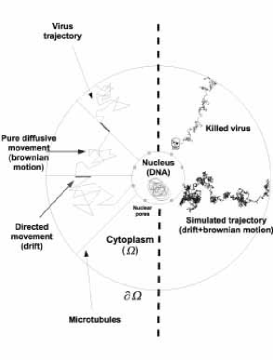
Figure 1: On the left-side of the idealized cell, a real trajectory consists of intermittent Brownian and drift epochs, whereas on the right-side, we show two simulated homogenized trajectories. In one of them, the virus arrives alive to a nuclear pore, while in the other, it is killed inside the cytoplasm. The round dots on the nucleus surface represent the nuclear pores.

From trajectory description to the probability and mean arrival time. Viral killing, immobilization or rejection out of the cell and naked DNA degradation by nucleases, are coarse-grained into a steady state killing rate $k$. To derive asymptotic expressions for the probability $P_{N}$, that a DNA carrier (single virus or DNA) arrives to a small nuclear pore alive and for the mean time $\tau_{N}$, we use the approximation (2). The asymptotic estimates depend on the diffusion constant $D$, the amplitude of the drift $B$, and $k$. These computations are based on the small hole theory [14], which describes a Brownian particle confined to a bounded domain by a reflecting boundary, except for a small absorbing window, through which it escapes. The domain $\Omega$ contains a spherical nucleus of small radius $\delta$. The survival probability density function (SPDF) $p(\mathbf{x},t)$ to find the virus or naked DNA alive inside the volume element $\mathbf{x}+d\mathbf{x}$ at time $t$ is given by

$$p(\mathbf{x},t)d\mathbf{x}=Pr\{X(t)\in\mathbf{x}+d\mathbf{x},\tau^{k}>t,\tau^{a}>t|p_{i}\},$$ (5)

where $\tau^{a}$ is the first passage time of a live DNA carrier to the absorbing boundary $\partial N_{a}$, $\tau^{k}$ is the first time it is hydrolyzed, and $p_{i}$ is the initial distribution. The SPDF $p(\mathbf{x},t)$ of the motion (3) is the solution of the mixed initial boundary value problem for the Fokker-Planck equation (FPE) [15]

$$\frac{\partial p}{\partial t}(\mathbf{x},t) = D\Delta p(\mathbf{x},t)-\nabla\cdot\mathbf{b}(\mathbf{x})p(\mathbf{x},t)-kp(\mathbf{x},t)$$

$$p(\mathbf{x},0) = p_{i}(\mathbf{x})\quad\mbox{for}\quad\mathbf{x}\in\Omega$$

$$p(\mathbf{x},t) = 0\quad\mbox{for}\quad\mathbf{x}\in\partial N_{a}$$

$$\mathbf{J}(\mathbf{x},t)\cdot\mathbf{n}_{\mathbf{x}} = 0\quad\mathbf{x}\in\partial N_{r}\cup\partial\Omega_{ext},$$

where $\mathbf{n}_{\mathbf{x}}$ is the unit outer normal at a boundary point $\mathbf{x}$. The flux density vector $\mathbf{J}(\mathbf{x},t)$ is defined as

$$\mathbf{J}(\mathbf{x},t)=-D\nabla p(\mathbf{x},t)+\mathbf{b}(\mathbf{x})p(\mathbf{x},t).$$ (6)

The probability $P_{N}$ that a live DNA carrier arrives at the nucleus is $P_{N}=Pr\{\tau^{a}<\tau^{k}\}$ [16]. This probability can be expressed in terms of the SPDF [16] by

$$P_{N}=1-Pr\{\tau^{a}>\tau^{k}\} = 1-\int_{\Omega}k(\mathbf{x})\tilde{p}(\mathbf{x})\,d\mathbf{x},$$

where $\tilde{p}(\mathbf{x})=\int_{0}^{\infty}p(\mathbf{x},t)\,dt$ is the solution of equation

$$qD\Delta\tilde{p}(\mathbf{x})-\nabla\cdot\mathbf{b}(\mathbf{x})\tilde{p}(\mathbf{x})-k(\mathbf{x})\tilde{p}(\mathbf{x})=-p_{i}(\mathbf{x})\quad\hbox{for}\quad\mathbf{x}\in\Omega$$ (7)

q with the boundary conditions (Introduction). Using the pdf of the time to absorption, conditioned on the event that the DNA carrier escapes alive $\Pr\{\tau^{a}<t\,|\,\tau^{a}<\tau^{k}\}$, we define the conditional mean time to absorption as

$$\tau_{N} = E[\tau^{a}\,|\,\tau^{a}<\tau^{k}]=\int_{0}^{\infty}{(1-\Pr\{\tau^{a}<t\,|\,\tau^{a}<\tau^{k})}\,dt.$$

Following the computations of [17], we get

$$\tau_{N}=\frac{\int_{\Omega}\tilde{p}(\mathbf{x})d\mathbf{x}-\int_{\Omega}k(\mathbf{x})q(\mathbf{x})d\mathbf{x}}{1-\int_{\Omega}k(\mathbf{x})\tilde{p}(\mathbf{x})\,d\mathbf{x}},,$$ (8)

where

$$q(\mathbf{x})=\int_{0}^{\infty}s\tilde{p}(\mathbf{x},s)\,ds$$ (9)

satisfies [17]

$$-\tilde{p}=D\Delta q(\mathbf{x})-\nabla\cdot\mathbf{b}q]-kq\quad\hbox{for}\quad\mathbf{x}\in\Omega$$ (10)

with boundary conditions (Introduction).

Asymptotic expressions: the plasmid case. To obtain explicit expression for $P_{N}$ and $\tau_{N}$ for a nucleus containing $n$ well separated small holes (nuclear pores) on its surface, we consider first a killing rate $k$ smaller than the diffusion constant $D$. The asymptotic analysis for naked DNA $(\mathbf{b}=\mathbf{0})$ leads to [17]

$$P_{N}=\frac{1}{1+\frac{|\Omega|\tilde{k}}{4nD\eta}},\quad\tau_{N}=\frac{\left(\frac{|\Omega|}{4D\eta n}\right)}{1+\left(\frac{|\Omega|\tilde{k}}{4nD\eta}\right)},$$ (11)

where $\tilde{k}=\frac{1}{|\Omega|}\int_{\Omega}k(\mathbf{x})\,d\mathbf{x}$, and $\eta$ is the radius of a small absorbing disk. Formula (11) does not depend on the specific shape of the killing rate $k$, but rather on its integral. We compare this asymptotic formula with Brownian simulations obtained for parameters $R=20\mu m$; $\delta=\frac{R}{5}$; $\eta=\delta\frac{\pi}{12}=1.05\mu m$; $k=\frac{1}{3600}s^{-1}$ [18]; $D=0.02\mu m^{2}s^{-1}$ [9]; $n=1,$ (a single big hole). This simulation corresponds to a cell with $2\%$ of the nuclear surface occupied by a large nuclear pore, or equivalently, to a simulation with $n=2000$ pores of radius $25nm$[19]. Because formula (11) depends only on the product $n\eta$, both simulations give the same result.

Time and Probability	$\tau_{N}$	$P_{N}$
Theoretical values	$3567s$	$0.90\%$
Simulated values (2000 particles.)	$3564s$	$0.97\%$

When $k(\mathbf{x})$ is much larger compared to diffusion, a boundary layer analysis leads to the asymptotic expression

$$P_{N}=\frac{n\eta|\partial\Omega|}{|\Omega|}\sqrt{\frac{D}{k_{0}}},$$

where we assume that the smooth killing rate is a constant $k_{0}$ in the neighborhood of the nuclear surface. Asymptotic expressions: the virus case. For a virus trajectory governed by equation (3), with a constant scalar drift $B$, the leading order term of the probability and the mean time are given by [17]

$$P_{N}=\frac{1}{\frac{\pi}{nD\eta}\left(\frac{D}{B}\delta^{2}+2\left(\frac{D}{B}\right)^{2}\delta+2\left(\frac{D}{B}\right)^{3}\right)k+1}\\ \tau_{N}=\frac{\frac{\pi}{nD\eta}\left(\frac{D}{B}\delta^{2}+2\left(\frac{D}{B}\right)^{2}\delta+2\left(\frac{D}{B}\right)^{3}\right)}{\frac{\pi}{nD\eta}\left(\frac{D}{B}\delta^{2}+2\left(\frac{D}{B}\right)^{2}\delta+2\left(\frac{D}{B}\right)^{3}\right)k+1}.$$

These asymptotic formulas show that the main contribution to the probability and the mean time comes from a boundary layer located near the nucleus surface. The killing rate $k$ in this case is the averaged value of the killing field in that boundary layer [17]. In figure 2, we compare the probability to arrive alive at the pore and the mean arrival time for several values of the drift and the constant killing rate.

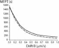
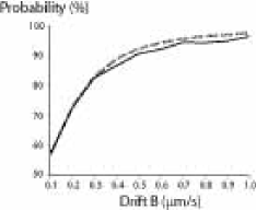
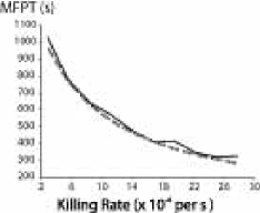
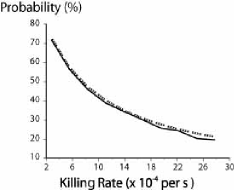
Figure 2: MFPT (top left) and the arrival probability (top right) for increasing values of the drift with $k=\frac{1}{3600}s^{-1}$ and for increasing values of the steady state killing rate ($B=0.2\mu ms^{-1}$) (bottom). $2000$ trajectories are simulated, theoretical values and simulated ones are drawn with dashed and solid lines, respectively. $R=20\mu m$; $\delta=4\mu m$; $\eta=\frac{\pi}{12}\delta=1.05\mu m$; $D=1.3\mu m^{2}s^{-1}$[4]; $n=1$.

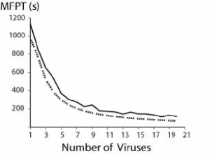
Figure 3: MFPT of the first virus. $300$ trajectories are simulated (solid line). $R=20\mu m$; $\delta=4\mu m$; $\eta=\frac{\pi}{12}\delta=1.05\mu m$; $D=1.3\mu m^{2}s^{-1}$; $n=1$ and $B=0.2\mu ms^{-1}$.

For a large number of microtubules, the drift $B$ equals the apparent velocity [13] ($10\%$ [20] of the minus end velocity, approximatively equal to $2\mu m/s$ [4]). Using formula (Introduction), we can now predict the effect of changing the effective drift $B=0.2$ by $\pm 30\%$: increasing the drift leads to a probability $P^{+30\%}_{N}=0.80$ and a mean time $\tau^{+30\%}_{N}=731s$, while reducing the drift gives $P^{-30\%}_{N}=0.64$ and $\tau^{-30\%}_{N}=1293s$. We conclude that decreasing the drift increases the time by $33\%$ ($\tau_{N}=974s$) and decreases the probability by $12\%$ ($P_{N}=0.73$), while increasing the drift, reduces the time by $22\%$ and increases the probability by $10\%$. These results show the nonlinear effect of the drift. In a biological context, decreasing the drift can be implemented by disrupting the microtubule network.

Mean first passage time of the first virus to reach the nucleus. When $M$ viruses enter a cell, the number $M_{a}$ of live viruses arriving at the nucleus is given by $M_{a}=P_{N}M$. The mean time the first live virus arrives at a nuclear pore is given by

$$\tau_{first}(M)=\frac{\tau_{N}}{1-\mathbf{x}i^{M}}\left(\sum_{k=0}^{M-1}\frac{\mathbf{x}i^{k}}{M-k}+\mathbf{x}i^{M}\sum_{k=1}^{M}\frac{\left(-1\right)^{k}}{k}\right)$$ (12)

where $\mathbf{x}i=1-P_{N}$. Finally, asymptotic expansions give

$$\tau_{first} \approx \left\{\begin{array}[]{l}\frac{\tau_{N}}{M}\left(1+\frac{M}{M-1}\mathbf{x}i\right)\hbox{ for }\mathbf{x}i\ll 1\\ \\ \frac{ln(\frac{M}{2})}{M}\frac{\tau_{N}}{1-\mathbf{x}i}\hbox{ for }\mathbf{x}i\approx 1\hbox{ and }M>>1.\end{array}\right.$$

The theoretical results are compared with Brownian simulations in figure 3.

The closed form expressions 11-Introduction facilitate the exploration of the multi-dimensional parameter space of cellular delivery of both DNA and virus trafficking. Cytoplasmic trafficking is a limiting step of gene delivery. Elucidating viral motion in the cytoplasm may provide a quantitative tool for the improvement and optimization of delivery of synthetic vectors. The present approach can provide a resource for optimizing the design of synthetic vectors and for the analysis of the parameters of viral infection.

References

- [1] M. Farquhar, G. Palade, Trends Cell Biol. 8, 2 (1998).
- [2] U.F. Greber, Cell. 124, 741 (2006).
- [3] N. Arhel et al., Nature Methods 3, 817 (2006).
- [4] G. Seisengerger et al., Science 294, 1929 (2001).
- [5] G. Zuber et al., Adv Drug Deliv Rev. 52, 245 (2001).
- [6] F. Nedelec, T.Surrey, A.C. Maggs, Phys Rev Lett. 86, 3192 (2001).
- [7] C. Pangarkar A.T. Dinh, S. Mitragotri, Phys Rev Lett. 95, 158101 (2005).
- [8] A.S. Verkman, Trends Biochem. Sci. 27, 27 (2002).
- [9] E. Dauty and A.S. Verkman, J. Biol. Chem. 280, 7823 (2005).
- [10] B. Sodeik, Trends Microbiol. 8, 465 (2000).
- [11] A.T. Dinh et al., Biophys. J. 92, 831 (2006).
- [12] M.A. Welte, Curr. Biol. 14, R525 (2004).
- [13] T. Lagache, D. Holcman (to be published).
- [14] D. Holcman and Z. Schuss, J. of Stat. Phys. 117, 975 (2004).
- [15] Z. Schuss, Theory and Applications of Stochastic Differential Equations (John Wiley, 1980).
- [16] D. Holcman, A. Marchewka, Z. Schuss, Phys. Rev. E 72, 031910 (2005).
- [17] D. Holcman, J. of Statistical Physics,127, 3 (2007).
- [18] Lechardeur et al. Gene Therapy, 6, 482 (1999).
- [19] G. Maul and L. Deaven, J. Cell Biol., 73, 748 (1977).
- [20] M. Suomalainen et .al J Cell Biol., 144, 657 (1999).