Implication of the Mott-limit violation in high-$T_{c}$ cuprates

Abstract

The Fermi arc is a striking manifestation of the strong-correlation physics in high-$T_{c}$ cuprates. In this paper, implications of the metallic transport in the lightly hole-doped regime of the cuprates, where the Fermi arcs are found, are examined in conjunction with competing interpretations of the Fermi arcs in terms of small hole pockets or a large underlying Fermi surface. It is discussed that the latter picture provides a more natural understanding of the metallic transport in view of the Mott-limit argument. Furthermore, it is shown that a suitable modeling of the Fermi arcs in the framework of the Boltzmann theory allows us to intuitively understand why the transport properties are apparently determined by a “small” carrier density even when the underlying Fermi surface, and hence $k_{F}$, is large.

I Introduction

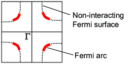
Figure 1: Schematic picture of the Fermi arcs observed in lightly-doped LSCO.

High-$T_{c}$ superconductivity shows up when carriers are doped to parent Mott-insulating cuprates where the energy gap opens due to strong electron correlations, i.e., strong Coulomb repulsions between electrons. It remains unsolved what exactly happens to the electronic structure when a small number of holes are introduced into the Mott-insulating state, although it is intuitively expected that such holes can move around and give rise to some charge conductivity; indeed, cuprates show a metallic transport behavior at moderate temperature upon slight hole doping. mobility Recent progress in the angle-resolved photoemission spectroscopy (ARPES) experimentsYoshida1 ; Yoshida2 ; ARPES has elucidated that an unusual electronic structure called “Fermi arcs” are formed in the Brillouin zone at the Fermi energy (see Fig. 1) when the metallic transport emerges in the lightly hole-doped cuprates. For example, in La_2-xSr_xCuO₄ (LSCO) with $x$ = 0.03, where a metallic transport is observed down to $\sim$70 K (see Fig. 2), a well-defined quasiparticle-like peak is observed in a limited loci in the Brillouin zone, which defines the Fermi arc;Yoshida1 intriguingly, these loci lie on the putative non-interacting Fermi surface that would be realized in the absence of strong correlations. Since the Fermi arc starts and ends in the middle of the Brillouin zone, it is not straightforward to apply such basic notion as the Luttinger sum ruleLuttinger that holds in ordinary Fermi liquids. Therefore, the Fermi arc is a striking manifestation of the new physics that stems from the strong electron correlations in hole-doped cuprates, and its understanding is obviously an important step towards understanding the high- $T_{c}$ superconductivity.

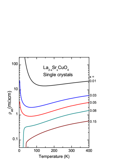
Figure 2: Temperature dependences of $\rho_{ab}$ of a series of high-quality LSCO single crystals measured up to 400 K. Note that a metallic behavior ($d\rho_{ab}/dT>0$) is observed at moderate temperature in all these samples, even for $x$ = 0.01.

Currently, there are essentially two schools of thoughts to interpret the Fermi arcs:ARPES One is to assume that the hole doping creates small (closed) hole pockets, but only a half of the pocket can be seen by ARPES due to a peculiar coherence factor of the strongly-correlated state. Chubukov ; Chakravarty ; Lee The other is to consider that there is a large inherent Fermi surface that is screwed due to the strong correlations, and asserts that only a portion of this large Fermi surface gains a spectral weight upon slight hole doping and forms the Fermi arcs. Norman ; Yang ; Tohyama ; Markiewicz ; Stanescu It would be very useful if one could elucidate which of the two is likely to be valid in view of the available transport data. In this article, I will try to make a case for the large Fermi surface picture based on the Mott-limit argument. Note, however, that those two pictures both implicitly assume that the system is uniform, and it will be a different story if the electrons develop a self-organized inhomogeneity in the lightly hole-doped cuprates. Zaanen ; Machida ; Muller ; anisotropy ; Kivelson

II Mott Limit and $k_{F}\ell$

An important principle for discussing whether a system should be a metal or an insulator is the Mott limit (or Mott-Ioffe-Regel limit),Mott which is based on very simple physics: For the metallic transport to be realized in a crystalline system, the Bloch waves of the electrons near the Fermi energy $\varepsilon_{F}$ must be well-defined, which dictates that their mean free path $\ell$ must be longer than the wave length $\lambda_{F}$ ($=2\pi/k_{F}$). This condition leads to the Mott limit that is expressed as $\ell\gtrsim\lambda_{F}$, which is equivalent to $k_{F}\ell\gtrsim 2\pi$. Since this argument is quite crude, it is customary to relax the condition a little and consider the Mott limit to be given by

$$k_{F}\ell\gtrsim 1.$$ (1)

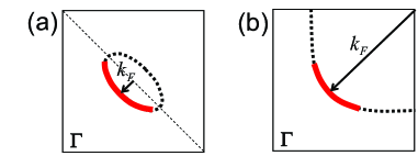
Figure 3: The Fermi wave vector $k_{F}$ associated with the Fermi arc in (a) the small hole pocket picture and (b) the large Fermi surface picture. Here, only a quarter of the 1st Brillouin zone is shown.

A prominent difference between the small hole pocket picture and the large Fermi surface picture for the Fermi arc is that the former gives a small $k_{F}$, while the latter dictates that $k_{F}$ must be large, as shown in Fig. 3. (Note that, for the discussion of the charge transport by holes, $k_{F}$ should be measured from the top of the relevant band.) To examine the metallic transport in LSCO shown in Fig. 2, let us try to estimate the electron mean free path $\ell$ by using the simple Drude theory, which gives the following expression for the resistivity:

$$\rho=\frac{c_{0}m^{*}}{e^{2}n_{\rm 2D}\tau},$$ (2)

where $m^{*}$ is the electron effective mass and $\tau$ is the relaxation time. Note that in the present case we consider a layered quasi-two-dimensional system with the layer distance $c_{0}$, and the resistivity $\rho$ is measured in the three-dimensional (3D) unit $\Omega$cm. To calculate $\tau$ from $\rho$ we need the carrier density $n_{\rm 2D}$, and we assert that it is the carrier density suggested by the Hall coefficient that should be used for this calculation. This is because in the lightly hole-doped regime (0.01 $\leq x\leq$ 0.05), as was demonstrated in Ref. AndoHall, , the Hall coefficient $R_{H}$ is nearly constant at moderate temperature (see Fig. 4) and its value agrees very well with $c_{0}/n_{\rm 2D}^{\rm nominal}e$, where $n_{\rm 2D}^{\rm nominal}=x/a^{2}$ and $a\simeq$ 3.8 Å is the in-plane lattice constant. (It is shown in the next section that, based on the Boltzmann theory, one should use the “small” $n_{\rm 2D}$ for this calculation even within the large Fermi surface picture.)

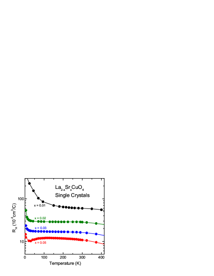
Figure 4: Temperature dependences of $R_{H}$ of high-quality LSCO single crystals in the lightly-doped regime ($x=0.01-0.05$) measured up to 400 K. Note that $R_{H}$ is essentially $T$-independent at moderate temperature, and its value agrees very well with $c_{0}/n_{\rm 2D}^{\rm nominal}e$ (= $a^{2}c_{0}/xe$), suggesting that a small carrier density $n_{\rm 2D}^{\rm nominal}$ is actually determining the transport properties.

In the small hole pocket picture, one may use the conventional formula $k_{F}=\sqrt{2\pi n_{\rm 2D}}$ for the two-dimensional (2D) system, which, together with $\ell=v_{F}\tau=(\hbar k_{F}\tau)/m^{*}$, leads to the simple, well-known formula

$$k_{F}\ell=(hc_{0})/(e^{2}\rho).$$ (3)

In the most extreme case of $x$ = 0.01, $\rho_{ab}$ at 300 K is 20 m$\Omega$cm (see Fig. 2), which gives $k_{F}\ell\simeq$ 0.1 according to Eq. (3). Obviously, the Mott limit Eq. (1) is strongly violated in this picture.

On the other hand, in the large Fermi surface picture, one may use the value $k_{F}\simeq$ 0.6 Å^-1 suggested by the ARPES data.Yoshida1 One may also adopt the $v_{F}$ value from ARPES experiments which found universal $v_{F}$ of $\sim$1.5 eVÅ that is nearly independent of doping.Yoshida2 Together with the estimate $m^{*}\simeq 3m_{e}$ ($m_{e}$ is the free electron mass) based on optical conductivity studies,Padilla in this picture $\rho_{ab}$(300 K) of 20 m$\Omega$cm would lead to $\tau\simeq$ 5 fs, which gives $\ell\simeq$ 10 Å and $k_{F}\ell\simeq$ 6. This satisfies the Mott limit and, hence, the metallic transport in the lightly hole-doped regime is naturally understood. Therefore, the fact that a metallic transport is realized at moderate temperature even at $x$ = 0.01 points to the conclusion that the large Fermi surface picture is the more appropriate one, while the small hole pocket picture bears a paradox.

III Fermi Arcs in the Framework of the Boltzmann Theory

Let us now discuss how the Boltzmann transport theoryZiman should be applied to the system that has Fermi arcs instead of an ordinary Fermi surface. First, one should remember that in the Boltzmann theory the charge current $\mathbf{J}$ is calculated as

$$\mathbf{J}=2\int_{{\rm all\ \mathbf{k}\ states}}e\mathbf{v_{k}}g_{\mathbf{k}}d^{3}\mathbf{k},$$ (4)

where $g_{\mathbf{k}}\equiv f_{\mathbf{k}}-f_{\mathbf{k}}^{0}$ is the deviation of the distribution function $f_{\mathbf{k}}$ from its equilibrium $f_{\mathbf{k}}^{0}$. When $g_{\mathbf{k}}$ is caused by the action of an electric field $\mathbf{E}$, in the relaxation time approximation $\mathbf{J}$ can be written as

$$\mathbf{J} = \frac{1}{4\pi^{3}}\int e^{2}\tau_{\mathbf{k}}\mathbf{v_{k}}(\mathbf{v_{k}}\cdot\mathbf{E})\left(-\frac{\partial f_{\mathbf{k}}^{0}}{\partial\varepsilon}\right)\frac{dS}{\hbar v_{\mathbf{k}}}d\varepsilon$$ (5)

$$= \frac{e^{2}}{4\pi^{3}\hbar}\int_{\rm FS}\tau_{\mathbf{k}}(\varepsilon_{F})v_{\mathbf{k}}\left(\frac{\mathbf{v}_{\mathbf{k}}}{v_{\mathbf{k}}}\cdot\mathbf{E}\right)dS_{F}.$$ (6)

It should be noted that $\partial f_{\mathbf{k}}^{0}/\partial\varepsilon$ in Eq. (5) is non-zero only near the Fermi surface, and this is why the surface integral on the Fermi surface appears in Eq. (6). The special care we take in the present calculation to accommodate the Fermi arc picture is that we allow the relaxation time $\tau_{\mathbf{k}}$ to vary over the Fermi surface.

Assume that $\mathbf{E}$ is along the $x$ axis. For a 2D system, one obtains from Eq. (6) that

$$J_{x} = \frac{e^{2}}{4\pi^{3}\hbar}\int_{\rm FS}\tau_{\mathbf{k}}(\varepsilon_{F})(v_{x}^{2}E_{x}/v)dL_{F}$$ (7)

$$= \frac{e^{2}}{8\pi^{3}\hbar}v_{F}E_{x}\int_{\rm FS}\tau_{\mathbf{k}}(\varepsilon_{F})dL_{F},$$ (8)

where $v=(v_{x}^{2}+v_{y}^{2})^{1/2}$ and $dL_{F}$ is the line element of the Fermi “surface” in the 2D Brillouin zone.

Adopting the large Fermi surface picture implies that one accepts the existence of an underlying large Fermi surface, across which the occupation number of the electronic states changes from one to zero. In order to incorporate the Fermi arcs in the above framework of the Boltzmann theory, one may suppose that only on the “arc” portion of the underlying large Fermi surface, $\tau_{\mathbf{k}}$ is long enough ($\tau_{\mathbf{k}}=\tau_{\rm arc}$) to allow well-defined quasiparticles. Furthermore, one may suppose $\tau_{\mathbf{k}}$ = 0 elsewhere on the underlying Fermi surface, which means that the states outside the Fermi arcs are incoherent. It should be remembered that upon performing the energy integral in Eq. (5) to derive Eq. (6), we relied on the fact that $\partial f_{\mathbf{k}}^{0}/\partial\varepsilon$ is non-zero only near the Fermi surface; the property $\partial f_{\mathbf{k}}^{0}/\partial\varepsilon\neq 0$ still holds at the underlying Fermi surface even when there are no well-defined quasiparticles on it (such a surface is called “Luttinger surface” in the recent literatureDzyaloshinskii ; Phillips ), so Eq. (8) is still valid in this picture.

With the above modeling of the Fermi arcs, one obtains the conductivity on the Fermi arc as

$$\sigma_{x}^{\rm arc} = \frac{e^{2}}{8\pi^{3}\hbar}v_{F}\int_{\rm FS}\tau_{\mathbf{k}}(\varepsilon_{F})dL_{F}$$ (9)

$$= \frac{e^{2}}{8\pi^{3}\hbar}v_{F}\tau_{\rm arc}\cdot L_{\rm arc},$$ (10)

where $L_{\rm arc}$ is the total length of the Fermi arcs. If the large Fermi surface is recovered (i.e., the arcs touch the Brillouin zone boundary), the conductivity $\sigma_{x}^{\rm full}$ would be written as $\sigma_{x}^{\rm full}=(e^{2}/8\pi^{3}\hbar)v_{F}\tau_{\rm arc}\cdot L_{\rm full}$ ($L_{\rm full}$ is the total length of the underlying Fermi surface), so the conductivity of the Fermi arc system can be expressed as

$$\sigma_{x}^{\rm arc}=p\sigma_{x}^{\rm full},$$ (11)

where $p\equiv L_{\rm arc}/L_{\rm full}$. Since the ARPES data suggests that $p$ increases linearly with doping in the lightly-doped regime,Yoshida2 Eq. (11) allows us to understand why the “small” $n_{\rm 2D}$ determines the conductivity even when the underlying Fermi surface, and hence $k_{F}$, is large. Quantitatively, the total length of the actual Fermi arcs observed in the lightly-doped LSCO is about a factor of three too longYoshida2 to explain the measured $\rho_{ab}$ with the above simple formalism, which indicates that a more elaborate modeling of the Fermi arcs, such as a $\mathbf{k}$ dependence of $\tau_{\rm arc}$, is necessary for a more quantitative description; nevertheless, the present model allows an intuitive understanding of the transport involving the Fermi arcs in the framework of the conventional Boltzmann theory.

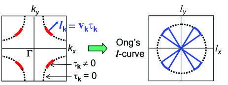
Figure 5: Schematic diagram of the Ong’s “l-curve” (Ref. OngHall, ) to calculate the Hall conductivity of the Fermi arc system in the framework of the Boltzmann theory. For simplicity, the underlying 2D Fermi surface is pictured as a simple circle.

As for the Hall conductivity $\sigma_{xy}$, the same modeling of the Fermi arcs leads to a simple result. For 2D metals, $\sigma_{xy}$ is most conveniently calculated by using the geometrical interpretation where $\sigma_{xy}$ is given by the “Stokes area” traced out by the l_k vector which defines the Ong’s “l-curve”.OngHall Since l${}_{\mathbf{k}}=\mathbf{v}_{\mathbf{k}}\tau_{\mathbf{k}}$, the l_k vector is non-zero only for those $\mathbf{k}$’s that are within the Fermi arcs (Fig. 5), and in the simplest case of a circular underlying Fermi surface and constant $\tau_{\mathbf{k}}$ on the Fermi arcs, one obtains $\sigma_{xy}^{\rm arc}=p\sigma_{xy}^{\rm full}$. In this case, the Hall coefficient can be written as

$$R_{H}^{\rm arc}=\frac{\sigma_{xy}^{\rm arc}}{(\sigma_{x}^{\rm arc})^{2}}=R_{H}^{\rm full}/p.$$ (12)

This essentially explains why the Fermi arcs can give rise to a Hall constant that reflects the “small” $n_{\rm 2D}$. Of course, for a really quantitative understanding, one needs a more elaborate modeling of the Fermi arcs.

IV Insulating Behavior

It is prudent to mention that the strong localization (or insulating) behavior is observed at low temperature in the lightly-doped regime. While at first sight it appears natural for the strong localization to occur when there are only a small number of carriers, when one calculates the $k_{F}\ell$ value at the onset of the localization, one finds it unusually large. For example, at $x$ = 0.05, $\rho_{ab}(T)$ shows strong localization below 50 K, where $\rho_{ab}$ = 0.9 m$\Omega$cm (see Fig. 2) and the corresponding $k_{F}\ell$ value is as large as 13. This is very unusual, because the strong localization is observed only when $k_{F}\ell<1$ in ordinary materials.Mott

Such an unusual nature of the localization in the lightly-doped regime is obviously related to the $\log(1/T)$ insulating behavior that shows up when the superconductivity is suppressed by high magnetic fields in underdoped LSCO,logT ; MI because the $k_{F}\ell$ value estimated by using Eq. (3) at the onset of the insulating behavior was as large as 13 for $x$ = 0.15.MI It is intriguing that the $\log(1/T)$ insulating behavior in LSCO has been observed for $x\leq$ 0.15,MI which exactly matches the doping range where the Fermi arcs are observed by ARPES.Yoshida2 This coincidence may imply that the Fermi arcs are inherently insulating at $T$ = 0 in the absence of superconductivity,Choy and the physical origin of the “insulating” behavior at large $k_{F}\ell$ values is an important remaining question.

V Summary

It is discussed that the large Fermi surface picture for the Fermi arcs allows us to understand the metallic transport observed at moderate temperature in the lightly hole-doped regime in a natural way; the small hole pocket picture, on the other hand, leads to a paradoxical conclusion of strong Mott-limit violation, as long as the system is considered to be uniform. Also, it is shown that the charge transport involving the Fermi arcs with large underlying Fermi surface can be understood in the framework of the conventional Boltzmann theory, by simply assuming that only on the Fermi arcs the quasiparticle lifetime is finite; furthermore, the proposed model allows us to intuitively understand why the “small” carrier density determines the transport properties even when $k_{F}$ is large.

- (1) Y. Ando, A. N. Lavrov, S. Komiya, K. Segawa, and X. F. Sun, Phys. Rev. Lett. 87, 017001 (2001).
- (2) T. Yoshida et al., Phys. Rev. Lett. 91, 027001 (2003).
- (3) T. Yoshida, X. J. Zhou, D. H. Lu, S. Komiya, Y. Ando, H. Eisaki, T. Kakeshita, S. Uchida, Z. Hussain, Z.-X. Shen, and A. Fujimori, J. Phys.: Condensed Matter 19, 125209 (2007).
- (4) A. Damascelli, Z. Hussain, and Z.-X. Shen, Rev. Mod. Phys. 75, 473 (2003).
- (5) J. M. Luttinger, Phys. Rev. 119, 1153 (1960).
- (6) A. V. Chubukov and D. K. Morr, Phys. Rep. 288, 355 (1997).
- (7) S. Chakravarty, C. Nayak, S. Tewari, Phys. Rev. B 68, 100504 (2003).
- (8) P. A. Lee, N. Nagaosa, and X.-G. Wen, Rev. Mod. Phys. 78, 17 (2006).
- (9) M. R. Norman et al., Nature 392, 157 (1998).
- (10) K.-Y. Yang, T. M. Rice, and F.-C. Zhang, Phys. Rev. B 73, 174501 (2006).
- (11) T. Tohyama, Phys. Rev. B 70, 174517 (2004).
- (12) R. S. Markiewicz, Phys. Rev. B 70, 174518 (2004).
- (13) T. D. Stanescu and G. Kotliar, Phys. Rev. B 74, 125110 (2006).
- (14) J. Zaanen and O. Gunnarsson, Phys. Rev. B 40, 7391 (1989).
- (15) K. Machida, Physica C 158, 192 (1989).
- (16) K. A. Müller, Physica C 341-348, 11 (2000).
- (17) Y. Ando, K. Segawa, S. Komiya, and A. N. Lavrov, Phys. Rev. Lett. 88, 137005 (2002).
- (18) S. A. Kivelson, I. P. Bindloss, E. Fradkin, V. Oganesyan, J. M. Tranquada, A. Kapitulnik, and C. Howald, Rev. Mod. Phys. 75, 1201 (2003).
- (19) N. F. Mott, Metal-Insulator Transitions (Taylor & Francis, London, 1990), 2nd ed.
- (20) Y. Ando, Y. Kurita, S. Komiya, S. Ono, and K. Segawa, Phys. Rev. Lett. 92, 197001 (2004).
- (21) W. J. Padilla, Y. S. Lee, M. Dumm, G. Blumberg, S. Ono, K. Segawa, S. Komiya, Y. Ando, and D. N. Basov, Phys. Rev. B 72, 060511(R) (2005).
- (22) A comprehensive description can be found in: J. M. Ziman, Principles of the Theory of Solids (Cambridge University Press, Cambridge, 1972), 2nd ed.
- (23) I. Dzyaloshinskii, Phys. Rev. B 68, 085113 (2003).
- (24) T. D. Stanescu, P. W. Phillips, and T.-P. Choy, Phys. Rev. B 75, 104503 (2007).
- (25) N. P. Ong, Phys. Rev. B 43, 193 (1991).
- (26) Y. Ando, G. S. Boebinger, A. Passner, T. Kimura, and K. Kishio, Phys. Rev. Lett. 75, 4662 (1995).
- (27) G. S. Boebinger, Y. Ando, A. Passner, T. Kimura, M. Okuya, J. Shimoyama, K. Kishio, K. Tamasaku, N. Ichikawa, and S. Uchida, Phys. Rev. Lett. 77, 5417 (1996).
- (28) T.-P. Choy and P. Phillips, Phys. Rev. Lett. 95, 196405 (2005).