INSTITUT NATIONAL DE RECHERCHE EN INFORMATIQUE ET EN AUTOMATIQUE

Towards Structural Classification of Proteins based on Contact Map Overlap
Rumen Andonov — Nicola Yanev — Noël Malod-Dognin N° 6370
Novembre 2007

Abstract: A multitude of measures have been proposed to quantify the similarity between protein 3-D structure. Among these measures, contact map overlap (CMO) maximization deserved sustained attention during past decade because it offers a fine estimation of the natural homology relation between proteins. Despite this large involvement of the bioinformatics and computer science community, the performance of known algorithms remains modest. Due to the complexity of the problem, they got stuck on relatively small instances and are not applicable for large scale comparison.

This paper offers a clear improvement over past methods in this respect. We present a new integer programming model for CMO and propose an exact B&B algorithm with bounds computed by solving Lagrangian relaxation. The efficiency of the approach is demonstrated on a popular small benchmark (Skolnick set, 40 domains). On this set our algorithm significantly outperforms the best existing exact algorithms, and yet provides lower and upper bounds of better quality. Some hard CMO instances have been solved for the first time and within reasonable time limits. From the values of the running time and the relative gap (relative difference between upper and lower bounds), we obtained the right classification for this test. These encouraging result led us to design a harder benchmark to better assess the classification capability of our approach. We constructed a large scale set of 300 protein domains (a subset of ASTRAL database) that we have called Proteus_300. Using the relative gap of any of the 44850 couples as a similarity measure, we obtained a classification in very good agreement with SCOP. Our algorithm provides thus a powerful classification tool for large structure databases.

Key-words: Protein structure alignment, Contact Map Overlap maximization, combinatorial optimization, integer programming, branch and bound, Lagrangian relaxation.

Vers une classification structurelle des protéines basée sur le recouvrement des cartes de contacts

Résumé : Une multitude de mesures ont été proposées pour quantifier la similarité entre les structures 3D de protéines. Parmis ces mesures, la maximisation du recouvrement des cartes de contacts ("Contact Map Overlap Maximization", CMO) a reçu durant les dix dernières années une attention soutenue, car elle permet une bonne estimation des relations naturelles d’homologie entre protéines. Cependant, malgré l’implication des communautés de bio-informatique et de sciences computationnelles, les performances des algorithmes connus restent modestes. À cause de la complexité du problème, ces algorithmes sont limités à de petites instances et ne sont pas applicables pour des comparaions à grandes échelles.

Ce rapport marque une nette amélioration sur ce point par rapport aux méthodes précedentes. Nous présentons un nouveau modèle de programmation linéaire en nombre entier pour CMO, et nous proposons un algorithme exact de séparation et évaluation dont les bornes proviennent de la relaxation lagrangienne de notre modèle. L’efficacité de cette approche est démontrée sur un petit ensemble de test connu (l’ensemble de skolnick, 40 domaines). Sur ce jeu de test, notre algorithme surpasse en rapidité d’exécution les meilleurs algorithmes existants tout en obtenant des bornes de meilleurs qualité. Quelques instances difficiles de CMO ont été résolues pour la première fois, et ce en des temps raisonnnables. À partir des valeurs de temps de calculs et de "gaps" relatifs (la différence relative entre la borne supérieur et inférieure), nous avons obtenu la bonne classification de l’ensemble de skolnick. Ces résultats encourageants nous ont poussés à créer un jeu de test plus difficile pour confirmer les capacités de classification de notre approche. Nous avons construit un ensemble de test contenant 300 domaines de protéines (un sous-ensemble d’ASTRAL) que nous avons appelé Proteus_300. En utilisant le gap relatif des 44850 couples comme une mesure de similarité, nous avons obtenu une classification en très bon accord avec SCOP. Notre algorithme offre donc un outil puissant pour la classification de grandes bases de données de structures.

Mots-clés : Alignement de structures de protéines, maximisation du recouvrement de cartes de contacts, optimisation combinatoire, programmation linéaire en nombre entier, séparation et évaluation, relaxation lagrangienne.

1 Introduction

A fruitful assumption of molecular biology is that proteins sharing close three-dimensional (3D) structures are likely to share a common function and in most case derive from a same ancestor. Computing the similarity between two protein structures is therefore a crucial task and has been extensively investigated [5, 14, 15, 22]. Interested reader can also refers [6, 7, 8, 9, 10, 11, 12, 18]. Since it is not clear what quantitative measure to use for comparing protein structures, a multitude of measures have been proposed. Each measure aims in capturing the intuitive notion of similarity. We studied the contact-map-overlap (CMO) maximization, a scoring scheme first proposed in [16]. This measure has been found to be very useful for estimating protein similarity - it is robust, takes partial matching into account, translation invariant and captures the intuitive notion of similarity very well. The protein’s primary sequence is usually thought as composed of residues. Under specific physiological conditions, the linear arrangement of residues will fold and adopt a complex 3D shape, called native state (or tertiary structure). In its native state, residues that are far away along the linear arrangement may come into proximity in 3D space. The proximity relation is captured by a contact map. Formally, a map is specified by a $0-1$ symmetric squared matrix $C$ where $c_{ij}=1$ if the Euclidean distance of two heavy atoms (or the minimum distance between any two atoms belonging to those residues) from the $i$-th and the $j$-th amino acid of a protein is smaller than a given threshold in the protein native fold. In the CMO approach one tries to evaluate the similarity of two proteins by determining the maximum overlap (also called alignment) of contacts map. Formally: given two adjacency matrices, find two sub-matrices that correspond to principle minors having the maximum inner product if thought as vectors (i.e. maximizing the number of 1 on the same position).

The counterpart of the CMO problem in the graph theory is the well known maximum common subgraph problem (MCS) [17]. The bad news for the later is its APX-hardness The only difference between the above defined CMO and MCS is that the isomorphism used for the MCS is not restricted to the non-crossing matching only. Nevertheless the CMO is also known to be NP-hard [13]. Thus the problem of designing efficient algorithms that guarantee the CMO quality is an important one that has eluded researchers so far. The most promising approach for solving CMO seems to be integer programming coupled with either Lagrangian relaxation [5] or B&B reduction technique [21].

The results in this paper confirm once more the superiority of Lagrangian relaxation to CMO since the algorithm we present belongs to the same class. Our interest in CMO was provoked by its similarity with the protein threading problem. For the later we have presented an approach based on the so called non-crossing matching in bipartite graphs [1]. It yielded a highly efficient algorithm solving the PTP by using the Lagrangian duality [2, 3, 4].

The contributions of this paper are as follows. We propose a new integer programming formulation of the CMO problem. For this model, we design a B&B algorithm coupled with a new Lagrangian relaxation for bounds computing. We compare our approach with the best existing exact algorithms [5, 21] on a widely used benchmark (the Skolnick set), and we noticed that it outperforms them significantly. New hard Skolnick set instances have been solved. In addition, we observed that our Lagrangian approach produces upper and lower bounds of better quality than in [5, 21]. This suggested us to use the relative gap (a function of these two bounds) as a similarity measure. To the best of our knowledge we are the first ones to propose such criterion for similarity. Our results demonstrated the very good classification potential of our method. Its capacity as classifier was further tested on the Proteus_300 set, a large benchmark of 300 domains that we extracted from ASTRAL-40 [23]. We are not aware of any previous attempt to use a CMO tool on such large database. The obtained classification is in very good agreement with SCOP classification. This clearly demonstrates that our algorithm can be used as a tool for large scale classification.

2 The mathematical model

We are going to present the CMO problem as a matching problem in a bipartite graph, which in turn will be posed as a longest augmented path problem in a structured graph. Toward this end we need to introduce few notations as follows. The contacts maps of two proteins P1 and P2 are given by graphs $G_{m}=(V_{m},E_{m})$ with $V_{m}=\{1,2,\ldots,n_{m}\}$ for $m=1,2$. The vertices $V_{m}$ are better seen as ordered points on a line and correspond to the residues of the proteins. The arcs $(i,j)$ correspond to the contacts. The right and left neighbouring of node $i$ are elements of the sets $\delta_{m}^{+}(i)=\{j|j>i,(i,j)\in E_{m}\}$, $\delta_{m}^{-}(i)=\{j|j<i,(j,i)\in E_{m}\}$. Let $i\in V_{1}$ be matched with $k\in V_{2}$ and $j\in V_{1}$ be matched with $l\in V_{2}$. We will call a matching non-crossing, if $i<j$ implies $k<l$. A feasible alignment of two proteins $P_{1}$ and $P_{2}$ is given by a non-crossing matching in the complete bipartite graph $B$ with a vertex set $V_{1}\cup V_{2}$.

Let the weight $w_{ikjl}$ of the matching couple $(i,k)(j,l)$ be set as follows

$$w_{ikjl}=\left\{\begin{array}[]{ll}1&\mbox{ if }(i,j)\in E_{1}\mbox{ and }(k,l)\in E_{2}\\ 0&\mbox{ otherwise}\end{array}\right.$$ (1)

For a given non-crossing matching $M$ in $B$ we define its weight $w(M)$ as a sum over all couples of edges in $M$. The CMO problem consists then in maximizing $w(M)$, where $M$ belongs to the set of all non-crossing matching in $B$.

In [1, 2, 3, 4] we have already dealt with non-crossing matching and we have proposed a network flow presentation of similar one-to-one mappings (in fact the mapping there was many-to-one). The adaptation of this approach to CMO is as follows: The edges of the bipartite graph $B$ are mapped to the points of $n_{1}\times n_{2}$ rectangular grid $B^{\prime}=(V^{\prime},E^{\prime})$ according to: point - $(i,k)\in V^{\prime}$ $\longleftrightarrow$ edge - $(i,k)$ in $B$.

Definition. The feasible path is an arbitrary sequence $(i_{1},k_{1}),(i_{2},k_{2}),\ldots,(i_{t},k_{t})$ of points in $B^{\prime}$ such that $i_{j}<i_{j+1}$ and $k_{j}<k_{j+1}$ for $j=1,2,\ldots,t-1$.

The correspondence feasible path $\leftrightarrow$ non-crossing matching is obvious. This way non-crossing matching problems are converted to problems on feasible paths. We also add arcs $(i,k)\rightarrow(j,l)\in E^{\prime}$ iff $w_{ikjl}=1$. In $B^{\prime}$, solving CMO corresponds to finding the densest (in terms of arcs) subgraph of $B^{\prime}$ whose node set is a feasible path (see Fig. 1).

Figure 1: Left: Vertex 1 from V1 is matched with vertex 1 from V2 and 2 is matched with 3: matching couple $(1,1)(2,3)$. Other matching couples are $(3,4)(5,5)$. This defines a feasible matching $M=\{(1,1)(2,3),(3,4)(5,5)\}$ with weight $w(M)=2$. Right: The same matching is visualized in graph $B^{\prime}$.

To each node $(i,k)\in V^{\prime}$ we associate now a $0/1$ variable $x_{ik}$, and to each arc $(i,k)\rightarrow(j,l)\in E^{\prime}$, a $0/1$ variable $y_{ikjl}$. Denote by $X$ the set of feasible paths. The problem can now be stated as follows (see Fig. 2 a) for illustration)

$$v(CMO)=\max\sum_{(ik)(jl)\in E^{\prime}}y_{ikjl}$$ (2)

subject to

$$x_{ik}\geq\sum_{l\in\delta_{2}^{+}(k)}y_{ikjl},\quad j\in\delta_{1}^{+}(i)\qquad\begin{array}[]{l}i=1,2,\dots,n1-1,\\ k=1,2,\ldots,n2-1\end{array}$$ (3)

$$x_{ik}\geq\sum_{l\in\delta_{2}^{-}(k)}y_{jlik},\quad j\in\delta_{1}^{-}(i)\qquad\begin{array}[]{l}i=2,3,\dots,n1,\\ k=2,3,\ldots,n2\end{array}$$ (4)

$$x_{ik}\geq\sum_{j\in\delta_{1}^{+}(i)}y_{ikjl},\quad l\in\delta_{2}^{+}(k)\qquad\begin{array}[]{l}i=1,2,\dots,n1-1,\\ k=1,2,\ldots,n2-1\end{array}$$ (5)

$$x_{ik}\geq\sum_{j\in\delta_{1}^{-}(i)}y_{jlik},\quad l\in\delta_{2}^{-}(k)\qquad\begin{array}[]{l}i=2,3,\dots,n1,\\ k=2,3,\ldots,n2.\end{array}$$ (6)

$$\begin{array}[]{l}x\in X\end{array}$$ (7)

Actually, we know how to represent $X$ with linear constraints. Recalling the definition of feasible path, (7) is equivalent to

$$\sum_{l=1}^{k}x_{il}+\sum_{j=1}^{i-1}x_{jk}\leq 1,\quad i=1,2,\ldots,n1,\quad k=1,2,\ldots,n2.$$ (8)

We recall that from the definition of the feasible paths in $B^{\prime}$ (non-crossing matching in $B$) the $j$-th residue from $P1$ could be matched with at most one residue from $P2$ and vice-versa. This explains the sums into right hand side of (3) and (5) – for arcs having their tails at vertex $(i,k)$; and (4) and (6)– for arcs heading to $(i,k)$. Any $(i,k)(j,l)$ arc can be activated ($y_{ikjl}=1$) iff $x_{ik}=1$ and $x_{jl}=1$ and in this case the respective constraints are active because of the objective function.

A tighter description of the polytope defined by (3)–(6) and $0\leq x_{ik}\leq 1$, $0\leq y_{ikjl}$ could be obtained by lifting the constraints (4) and (6) as it is shown in Fig. 2 b). The points shown are just the predecessors of $(i,k)$ in graph $B^{\prime}$ and they form a grid of $\delta_{1}^{-}(i)$ rows and $\delta_{2}^{-}(k)$ columns. Let $i_{1},i_{2},\dots,i_{s}$ be all the vertices in $\delta_{1}^{-}(i)$ ordered according the numbering of the vertices in $V_{1}$ and likewise $k_{1},k_{2},\dots,k_{t}$ in $\delta_{2}^{-}(k)$. Then the vertices in the $l$-th column $(i_{1},k_{l}),(i_{2},k_{l}),\dots(i_{s},k_{l})$ correspond to pairwise crossing matching and at most one of them could be chosen in any feasible solution $x\in X$ (see (6)). This "all crossing" property will stay even if we add to this set the following two sets: $(i_{1},k_{1}),(i_{1},k_{2}),\dots,(i_{1},k_{l-1})$ and $(i_{s},k_{l+1}),(i_{s},k_{l+2}),\dots,(i_{s},k_{t})$. Denote by $col_{ik}(l)$ the union of these three sets and analogously by $row_{ik}(j)$ the corresponding union for the $j$-th row of the grid. When the grid is one column/row only the set $row_{ik}(j)$/$col_{ik}(l)$ is empty.

Now a tighter LP relaxation of (3)–(6) is obtained by changing (4) with

$$x_{ik}\geq\sum_{(r,s)\in row_{ik}(j)}y_{rsik},\quad j\in\delta_{1}^{-}(i)\qquad\begin{array}[]{l}i=2,3,\dots,n1,\\ k=2,3,\ldots,n2\end{array}$$ (9)

and (6) with

$$x_{ik}\geq\sum_{(r,s)\in col_{ik}(l)}y_{rsik},\quad l\in\delta_{2}^{-}(k)\qquad\begin{array}[]{l}i=2,3,\dots,n1,\\ k=2,3,\ldots,n2.\end{array}$$ (10)

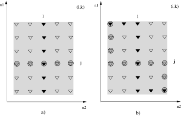
Figure 2: The shadowed area represents the set of vertices in $V^{\prime}$ which are tails for the arcs heading to $(i,k)$.  In a): $\blacktriangledown$ corresponds to the indices of $y_{jlik}$ in (6) for $l$ fixed. $\bigcirc$ corresponds to the indices of $y_{jlik}$ in (4) for $j$ fixed.  In b): $\blacktriangledown$ corresponds to the indices of $y_{jlik}$ in (10) for $l$ fixed (the set $col_{ik}(l)$). $\bigcirc$ corresponds to the indices of $y_{jlik}$ in (9) for $j$ fixed (the set $row_{ik}(j)$).

Remark: Since we are going to apply the Lagrangian technique there is no need neither for an explicit description of the set $X$ neither for lifting the constraints (3) (5).

3 Lagrangian relaxation approach

Here, we show how the Lagrangian relaxation of constraints (9) and (10) leads to an efficiently solvable problem, yielding upper and lower bounds that are generally better than those found by the best known exact algorithm [5].

Let $\lambda_{ikj}^{h}\geq 0$ (respectively $\lambda_{ikj}^{v}\geq 0$) be a Lagrangian multiplier assigned to each constraint (9) (respectively (10)). By adding the slacks of these constraints to the objective function with weights $\lambda$, we obtain the Lagrangian relaxation of the CMO problem

$$\begin{array}[]{ll}LR(\lambda)=&\displaystyle\max\sum_{i,k,j\in\delta_{1}^{-}(i)}\lambda_{ikj}^{h}(x_{ik}-\sum_{(r,s)\in row_{ik}(j)}y_{rsik})\\ &\displaystyle+\sum_{i,k,l\in\delta_{2}^{-}(k)}\lambda_{ikl}^{v}(x_{ik}-\sum_{(r,s)\in col_{ik}(l)}y_{rsik})+\sum_{(ik)(jl)\in E_{B^{\prime}}}y_{ikjl}\end{array}$$ (11)

subject to $x\in X$, (3), (5) and $y\geq 0$.

Proposition 1

$LR(\lambda)$ can be solved in $O(|V^{\prime}|+|E^{\prime}|)$ time.

Proof: For each $(i,k)\in V^{\prime}$, if $x_{ik}=1$ then the optimal choice $y_{ikjl}$ amounts to solving the following : The heads of all arcs in $E^{\prime}$ outgoing from $(i,k)$ form a $|\delta^{+}(i)|\times|\delta^{+}(k)|$ table. To each point $(j,l)$ in this table, we assign the profit $\max\{0,c_{ikjl}(\lambda)$}, where $c_{ikjl}(\lambda)$ is the coefficient of $y_{ikjl}$ in (11). Each vertex in this table is a head of an arc outgoing from $(i,k)$. Then the subproblem we need to solve consists in finding a subset of these arcs having a maximal sum $c_{ik}(\lambda)$ of profits(the arcs of negative weight are excluded as a candidates for the optimal solution) and such that their heads lay on a feasible path. This could be done by a dynamic programming approach in $O(|\delta^{+}(i)||\delta^{+}(k)|)$ time. Once profits $c_{ik}(\lambda)$ have been computed for all $(i,k)$ we can find the optimal solution to $LR(\lambda)$ by using the same DP algorithm but this time on the table of $n1\times n2$ points with profits for $(i,k)$-th one given by

$$c_{ik}(\lambda)+\sum_{j\in\delta_{1}^{-}(i)}\lambda_{ikj}^{h}+\sum_{l\in\delta_{2}^{-}(k)}\lambda_{ikl}^{v}.$$ (12)

where the last two terms are the coefficients of $x_{ik}$ in (11).

Remark: The inclusion $x\in X$ is explicitly incorporated in the DP algorithm.

3.1 The algorithm

In order to find the tightest upper bound on $v(CMO)$ (or eventually to solve the problem), we need to solve in the dual space of the Lagrangian multipliers $LD=\min_{\lambda\geq 0}LR(\lambda)$, whereas $LR(\lambda)$ is a problem in $x,y$. A number of methods have been proposed to solve Lagrangian duals: subgradient method, dual ascent methods,constraint generation method, column generation, bundel methods,augmented Lagrangian methods, etc. Here, we choose the subgradient method. It is an iterative method in which at iteration $t$, given the current multiplier vector $\lambda^{t}$, a step is taken along a subgradient of $LR(\lambda)$, then if necessary, the resulting point is projected onto the nonnegative orthant. It is well known that practical convergence of the subgradient method is unpredictable. For some problems, convergence is quick and fairly reliable, while other problems tend to produce erratic behavior of the multiplier sequence, or the Lagrangian value, or both. In a "good" case, one usually observe a saw-tooth pattern in the Lagrangian value for the first iterations, followed by a roughly monotonic improvement and asymptotic convergence to a value that is hopefully the optimal Lagrangian bound. The computational runs on a reach set of real-life instances confirm a "good" case belonging of our approach at some expense in the speed of the convergence.

In our realization, the update scheme for $\lambda_{ikj}$ is $\lambda_{ikj}^{t+1}=\max\{0,\lambda_{ikj}^{t}-\Theta^{t}g_{ikj}^{t}\}$ , where $g_{ikj}^{t}=\bar{x}_{ik}-\sum\bar{y}_{jlik}$ (see (9) and (10) for the sum definition) is the sub-gradient component ($0,1$,or $-1$), calculated on the optimal solution $\bar{x}$, $\bar{y}$ of $LR(\lambda^{t})$. The step size $\Theta^{t}$ is $\Theta^{t}=\frac{\alpha(LR(\lambda^{t})-Z_{lb})}{\sum(g_{ikj}^{t})^{2}+\sum(g_{ikl}^{t})^{2}}$ where $Z_{lb}$ is a known lower bound for the CMO problem and $\alpha$ is an input parameter. Into this approach the $x$-components of $LR(\lambda^{t})$ solution provides a feasible solution to CMO and thus a lower bound also. The best one (incumbent) so far obtained is used for fathoming the nodes whose upper bound falls below the incumbent and also in section 4 for reporting the final gap. If $LD\leq v(CMO)$ then the problem is solved. If $LD>v(CMO)$ holds, in order to obtain the optimal solution, one could pass to a branch&bound algorithm suitably tailored for such an upper bounds generator.

From among various possible nodes splitting rules, the one shown in Fig. 3 gives quite satisfactory results (see section 4). Formally, let the current node be a subproblem of CMO defined over the vertices of $V^{\prime}$ falling in the interval $[lc(k),uc(k)]$ for $k=1,n_{2}$ (in Fig. 3 these are the points in-between two broken lines (the white area). Let $(rowbest,colbest)$ be the $\arg\max\min(S_{u}(i,k),S_{d}(i,k))$, where $S_{d}(i,k)=\sum_{j\leq k}\max(uc(j)-i,0)$ and $S_{u}(i,k)=\sum_{j\geq k}\max(i-lc(j),0)$. Now, the two descendants of the current node are obtained by discarding from its feasible set the vertices in $S_{d}(rowbest,colbest)$ and $S_{u}(rowbest,colbest)$ respectively. The goal of this strategy is twofold: to create descendants that are balanced in sense of feasible set size and to reduce maximally the parent node’s feasible set.

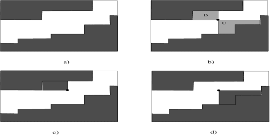
Figure 3: Sketch of the B&B splitting strategy.  a) the white area in-between broken lines represents the current node feasible set;  b) This set is split by $(rowbest,colbest)$, D corresponds to the set $S_{d}(rowbest,colbest)$ while U corresponds to the set $S_{u}(rowbest,colbest)$;  c) and d) are the descendants of the node a).

In addition, the following heuristics happened to be very effective during the traverse of the B&B tree nodes. Once the lower and the upper bound are found at the root node, an attempt to improve the lower bound is realized as follows.

Let $(i_{k_{1}},k_{1}),(i_{k_{2}},k_{2}),\dots,(i_{k_{s}},k_{s})$ be an arbitrary feasible path which activates certain number of arcs (recall that each iteration in the sub-gradient optimization phase generates such path and lower bound as well).

Then for a given strip size $sz$ (an input parameter set by default to $4$), the matchings in the original CMO are restricted to fall in a neighborhood of this path, allowing $x_{ik}$ to be non zero only for

$$\max\{1,i_{j}-sz\}\leq i\leq\min\{n1,i_{j}+sz\},j=k_{1},k_{2},\dots,k_{s}.$$

The Lagrangian dual of this subproblem is solved and a better lower bound is possibly sought. If the bound improves the incumbent, the same procedure is repeated by changing the strip alongside the new feasible solution.

Finally, the main steps of the B&B algorithm are as follows:
Initialization: Set $L$={original CMO problem, i.e. no restrictions on the feasible paths}.
Problem selection and relaxation: Select and delete the problem $P^{i}$ from $L$ having the biggest upper bound. Solve the Lagrangian dual of $P^{i}$. (Here a repetitive call to a heuristics is included after each improvement on the lower bound).
Fathoming and Pruning: Follow classical rules.
Partitioning : Create two descendants of $P^{i}$ using $(rowbest,colbest)$ and add them to $L$.
Termination : if $L=\emptyset$, the solution $(x^{*},y^{*})$ yielding the objective value is optimal.

4 Numerical results

To evaluate the above algorithm we performed two kinds of experiments. In the first one we compared our approach with the best existing algorithm from literature [5] in term of performance and quality of the bounds. This comparison was done on a set of proteins suggested by Jeffrey Skolnick which was used in various recent papers related to protein structure comparison [5, 18, 21]. This set contains 40 medium size domains from 33 proteins, which number of residues varies from 95 (2b3iA) to 252 (1aw2A). The maximum number of contacts is 593 (1btmA). We afterwards experimentally evaluated the capability of our algorithm to perform as classifier on the Proteus_300 set, a significantly larger protein set. It contains 300 domains, which number of residues varies from 64 (d15bba_) to 455 (d1po5a_). Its maximum number of contact is 1761 (d1i24a_). We will soon make available all data and results on the URL:
http://www.irisa.fr/symbiose/softwares/resources/proteus300

4.1 Performance and quality of bounds

The results presented in this section were obtained on machines with AMD Opteron(TM) CPU at 2.4 GHz, 4 Gb Ram, RedHat 9 Linux. The algorithm was implemented in C. According to SCOP classification [19], the Skolnick set contains five families (see Table  2 in Annexe). Note that both approaches that we compare use different Lagrangian relaxations. Our algorithm is called a_purva, while the other Lagrangian algorithm is denoted by LR.

The Skolnick set requires aligning 780 pairs of domains. We bounded the execution time to 1800 seconds for both algorithms. a_purva succeeded to solve 171 couples in the given time, while LR solved only 157 couples. Note that another exact algorithm called CMOS has been proposed in a very recent paper [21]. CMOS succeeded to solve only 161 instances from the Skolnick set, yet the time limit was 4 hours on a similar workstation. Hence it seems that 171 is the best score ever obtained when exactly solving Skolnick set. To the best of our knowledge, we are the first ones to solve all the 164 instances with couples from the same SCOP folds, as well as the first to solve instances with couples from different folds (the 7 instances of the $6^{th}$ class presented in Table LABEL:table-1). The interested reader can find our detailed results on the webpage cited before.

Figure 4 illustrates LR/a_purva time ratio as a function of solved instances. It is easily seen that a_purva is significantly faster than LR (up to several hundred times in the majority of cases). Table LABEL:table-1 in the Annexe contains more details concerning a subset of 164 pairs of proteins. We observed that this set is a very interesting one. It is characterized by the following properties: a) in all but the 6 last instances the a_purva running time is less than 10 seconds; b) in all instances the relative gap at the root of the B&B is smaller than 4, while in all other instances this gap is much larger (greater than 18 even for couples solved in less than 1800 sec); c) this set contains all instances such that both proteins belong to the same family according to SCOP classification. In other words, each pair such that both proteins belong to the same family is an easily solvable instance for a_purva and this feature can be successfully used as a discriminator. In fact, by virtue of this relation we were able to correctly classify the 40 items in the Skolnick set in 2000 seconds overall running time for all 780 instances. We will go back over this point in the next section.

Figure 4: $\frac{\mbox{LR time}}{\mbox{a\_purva time}}$ ratio as a function of solved instances

Our next observation (see Fig.  5 and Fig. 6 in the Annexe) concerns the quality of gaps obtained by both algorithms on the set of unsolved instances. Remember that when a Lagrangian algorithm stops because of time limit (1800 sec. in our case) it provides two bounds: one upper (UB), and one lower (LB). Providing these bounds is a real advantage of a B&B type algorithm compared to any meta-heuristics. These values can be used as a measure for how far is the optimization process from finding the exact optimum. The value UB-LB is usually called absolute gap. Any one of the 609 points $(x,y)$ in Fig.  5 presents the absolute gap for a_purva ($x$ coordinate) and for LR ($y$ coordinate) algorithm. All points are above the $y=x$ line (i.e. the absolute gap for a_purva is always smaller than the absolute gap for LR). On the other hand the entire figure is very asymmetric in a profit of our algorithm since its maximal absolute gap is 33, while it is 183 for LR.

In Fig. 6 we similarly compare lower and upper bounds separately. Any point $\circ$ has the lower bound computed by a_purva (res. LR) as $x$ (res. $y$) coordinate, while any point $\times$ has the upper bound computed by a_purva (res. LR) as $x$ (res. $y$) coordinate. We observe that in a large majority the points $\circ$ are below the $y=x$ line while the points $\times$ are above this line. This means that usually a_purva lowers bounds are higher, while its upper bounds are all smaller and therefore a_purva provides bounds with clearly better quality than LR. We don’t have much information about the bounds find by CMOS, except that at the root of the B&B tree, it obtains upper bounds of worst quality than the ones of LR.

Figure 5: Comparing absolute gaps on the set of unsolved instances. The gaps computed by a_purva are significantly smaller.

4.2 A_purva as a classifier

When running a_purva on the Skolnick set, we observed that relative gaps are smaller for similar domains than for dissimilar ones. This became even more obvious when we fixed a small upper bound of iterations and limited the computations only to the root of the B&B tree. The question then was to check if the relative gap can be used as a similarity index (the smaller is the relative gap, the more similar are the domains) which can be given to an automatic classifier in order to quickly provide a classification.

We used the following protocol : the runs of a_purva were limited to the root, with a limit of 500 iterations for the subgradient descent. We used the publicly available hierarchical ascendant classifier Chavl [20], which proposes a best partition of classified elements based on the derivative of the similarity index and thus requires no similarity threshold. For the Skolnick set, the alignment of all couples was done in less than 1100 seconds (with a mean computation time of 1.39 seconds/couple). The classification returned by Chavl based on the relative gap is exactly the classification at the fold level in SCOP. Taking into account that according to Table LABEL:table-1, 609 couples ran 1800 seconds without finding the solution, this result pushes to use the relative gap as a classifier. Note also that we succeeded to classify the Skolnick set significantly faster than both previously published exact algorithms [21, 5] that use similarity indexes based on lower bound only. This illustrates the effectiveness of using a similarity based on both upper and lower bounds.

To get a stronger confirmation of a_purva classifier capabilities, we performed the same operation on the Proteus_300 set, presented in Table LABEL:table-2. The alignment of the 44850 couples required roughly 82 hours (with a mean computation time of 6,58 seconds/couple).

Table LABEL:table-3 presents the classification that we obtain. It contains 25 classes denoted by letters A-Y. This classification is almost identical to the SCOP one (at folds level) which contains 24 classes denoted by numbers (presented in Table LABEL:table-2). 18 of the 24 SCOP classes correspond perfectly to our classes. Class 15 (resp. 24) contains two families that we classified in M and N (resp. V and W). Classes 9 and 11 were merged into class I and are indeed similar, with some domains (like d1jgca_ and d1b0b__) having more than 75% of common contacts. Class 18 was split into its two families (X and Y), but Y was merged with class 10. Again, some of the corresponding domains (e.g. d1b00a_ and d1wb1a4) are very similar, with more than 75% of common contacts.

5 Conclusion

In this paper, we give an efficient exact B&B algorithm for contact map overlap problem. The bounds are found by using Lagrangian relaxation and the dual problem is solved by sub-gradient approach. The efficiency of the algorithm is demonstrated on a benchmark set of 40 domains and the dominance over the existing algorithms is total. In addition,its capacity as classifier (and this was the primary goal) was tested on a large data set of 300 protein domains. We were able to obtain in a short time a classification in very good agreement to the well known SCOP database.

We are curently working on the integration of biological information into the contact maps, such as the secondary structure type of the residues (alpha helix or beta strand). Aligning only residues from the same type will reduce the research space and thus speed up the algorithm.

6 Acknowledgement

Supported by ANR grant Calcul Intensif projet PROTEUS (ANR-06-CIS6-008) and by Hubert Curien French-Bulgarian partnership “RILA 2006” N⁰ 15071XF.

N. Malod-Dognin is supported by Région Bretagne.

We are thankful to Professor Giuseppe Lancia for numerous discussions and for kindly providing us with the source code and the contact map graphs for the Skolnick set.

All computations were done on the Ouest-genopole bioinformatics platform (http://genouest.org).

Table 1: Column one contains the number of the families according to table 2. The sixth class contains the hardest solved Skolnick set intstances. Column two(six) contains the names of the couples, column three(seven) is the score, column four(height) gives the time in seconds taken by LR algoritm, and column five(nine) presents the corresponding time taken by a_purva.

F	Proteins	CMO	Time	Time	Proteins	CMO	Time	Time
	Name		LR	a_pr	Name		LR	a_pr
1	1b00A 1dbwA	149	192.00	1.2	1ntr_ 1qmpA	119	545.94	7.18
1	1b00A 1nat_	145	166.98	1.11	1ntr_ 1qmpB	115	454.01	4.23
1	1b00A 1ntr_	118	565.47	3.59	1ntr_ 1qmpC	116	610.93	6.56
1	1b00A 1qmpA	143	198.72	1.33	1ntr_ 1qmpD	118	522.53	4.44
1	1b00A 1qmpB	136	439.95	59.65	1ntr_ 3chy_	130	339.86	5.53
1	1b00A 1qmpC	139	263.81	1.68	1ntr_ 4tmyA	126	450.05	3.34
1	1b00A 1qmpD	137	181.23	1.89	1ntr_ 4tmyB	127	399.26	3.75
1	1b00A 3chy_	154	141.50	0.85	1qmpA 1qmpB	221	3.77	0.03
1	1b00A 4tmyA	155	143.92	0.9	1qmpA 1qmpC	232	0.35	0.02
1	1b00A 4tmyB	155	75.41	0.73	1qmpA 1qmpD	230	0.02	0.03
1	1dbwA 1nat_	157	226.42	1.51	1qmpA 3chy_	160	69.78	1.07
1	1dbwA 1ntr_	130	426.13	5.53	1qmpA 4tmyA	162	98.21	0.78
1	1dbwA 1qmpA	152	159.74	2.93	1qmpA 4tmyB	164	50.48	0.62
1	1dbwA 1qmpB	150	63.63	1.52	1qmpB 1qmpC	221	1.60	0.02
1	1dbwA 1qmpC	150	180.52	2.38	1qmpB 1qmpD	220	1.61	0.03
1	1dbwA 1qmpD	152	111.28	1.78	1qmpB 3chy_	156	68.17	0.84
1	1dbwA 3chy_	164	84.22	1.19	1qmpB 4tmyA	157	51.32	0.58
1	1dbwA 4tmyA	161	73.71	1.1	1qmpB 4tmyB	156	66.11	0.64
1	1dbwA 4tmyB	163	47.87	1.11	1qmpC 1qmpD	226	3.65	0.02
1	1nat_ 1ntr_	127	302.39	3.59	1qmpC 3chy_	157	75.14	1.23
1	1nat_ 1qmpA	157	66.03	1.04	1qmpC 4tmyA	162	55.46	1.26
1	1nat_ 1qmpB	149	69.00	0.99	1qmpC 4tmyB	162	78.52	0.58
1	1nat_ 1qmpC	152	73.53	1.07	1qmpD 3chy_	158	59.47	1.11
1	1nat_ 1qmpD	151	99.14	1.33	1qmpD 4tmyA	157	59.23	0.71
1	1nat_ 3chy_	163	76.95	0.86	1qmpD 4tmyB	159	53.27	0.59
1	1nat_ 4tmyA	175	15.58	0.28	3chy_ 4tmyA	171	54.33	0.55
1	1nat_ 4tmyB	172	19.06	0.37	3chy_ 4tmyB	174	41.43	0.5
1					4tmyA 4tmyB	230	0.02	0.02
2	1bawA 1byoA	152	11.59	0.25	1byoB 2b3iA	135	7.21	0.27
2	1bawA 1byoB	155	6.11	0.18	1byoB 2pcy_	175	2.28	0.05
2	1bawA 1kdi_	140	33.84	0.55	1byoB 2plt_	174	3.90	0.06
2	1bawA 1nin_	153	9.45	0.21	1kdi_ 1nin_	129	52.53	1.13
2	1bawA 1pla_	124	28.04	0.62	1kdi_ 1pla_	126	33.59	0.89
2	1bawA 2b3iA	130	15.57	0.38	1kdi_ 2b3iA	122	40.83	0.84
2	1bawA 2pcy_	148	6.91	0.16	1kdi_ 2pcy_	145	15.19	0.3
2	1bawA 2plt_	161	5.22	0.13	1kdi_ 2plt_	150	24.56	0.32
2	1byoA 1byoB	192	2.61	0.02	1nin_ 1pla_	130	22.76	0.69
2	1byoA 1kdi_	148	17.89	0.35	1nin_ 2b3iA	129	25.55	0.5
2	1byoA 1nin_	140	30.14	0.85	1nin_ 2pcy_	139	23.31	0.49
2	1byoA 1pla_	150	7.55	0.16	1nin_ 2plt_	146	18.85	0.52
2	1byoA 2b3iA	132	10.26	0.39	1pla_ 2b3iA	122	12.65	0.32
2	1byoA 2pcy_	176	2.18	0.04	1pla_ 2pcy_	143	4.75	0.14
2	1byoA 2plt_	172	3.77	0.07	1pla_ 2plt_	144	7.10	0.17
2	1byoB 1kdi_	152	11.89	0.21	2b3iA 2pcy_	127	11.79	0.35
2	1byoB 1nin_	141	21.05	0.6	2b3iA 2plt_	140	7.37	0.17
2	1byoB 1pla_	148	6.94	0.16	2pcy_ 2plt_	172	3.67	0.06
3	1amk_ 1aw2A	411	1272.28	1.48	1btmA 1tmhA	432	1801.97	2.81
3	1amk_ 1b9bA	400	1044.23	2.04	1btmA 1treA	433	1512.26	2.59
3	1amk_ 1btmA	427	1287.48	2.38	1btmA 1tri_	419	1455.08	3.26
3	1amk_ 1htiA	407	265.16	1.4	1btmA 1ydvA	385	692.72	1.52
3	1amk_ 1tmhA	424	638.26	1.29	1btmA 3ypiA	406	1425.09	2.43
3	1amk_ 1treA	411	716.51	1.52	1btmA 8timA	408	940.59	2
3	1amk_ 1tri_	445	447.54	0.97	1htiA 1tmhA	416	588.98	1.07
3	1amk_ 1ydvA	384	462.44	1.05	1htiA 1treA	426	395.23	0.81
3	1amk_ 3ypiA	412	427.66	0.97	1htiA 1tri_	412	779.84	1.55
3	1amk_ 8timA	410	386.73	0.94	1htiA 1ydvA	382	405.04	1.09
3	1aw2A 1b9bA	411	961.04	3.28	1htiA 3ypiA	422	148.75	0.56
3	1aw2A 1btmA	434	750.67	3.1	1htiA 8timA	463	112.65	0.52
3	1aw2A 1htiA	425	363.03	1.78	1tmhA 1treA	513	119.27	0.23
3	1aw2A 1tmhA	474	185.72	0.51	1tmhA 1tri_	413	630.57	2.19
3	1aw2A 1treA	492	157.79	0.37	1tmhA 1ydvA	384	785.56	1.5
3	1aw2A 1tri_	408	1313.53	3.51	1tmhA 3ypiA	417	766.79	2.11
3	1aw2A 1ydvA	386	650.55	1.62	1tmhA 8timA	421	516.44	1.47
3	1aw2A 3ypiA	401	895.17	2.28	1treA 1tri_	401	1169.41	2.68
3	1aw2A 8timA	423	276.06	1.76	1treA 1ydvA	389	1419.90	2.21
3	1b9bA 1btmA	441	653.29	2.08	1treA 3ypiA	407	522.65	1.34
3	1b9bA 1htiA	394	809.23	2.27	1treA 8timA	425	310.95	1.15
3	1b9bA 1tmhA	418	548.56	1.34	1tri_ 1ydvA	371	1040.31	1.92
3	1b9bA 1treA	410	613.99	1.25	1tri_ 3ypiA	412	607.52	1.75
3	1b9bA 1tri_	391	1804.98	3.32	1tri_ 8timA	412	830.38	1.45
3	1b9bA 1ydvA	362	1608.97	6.1	1ydvA 3ypiA	374	355.82	0.92
3	1b9bA 3ypiA	396	700.45	1.88	1ydvA 8timA	388	399.47	0.99
3	1b9bA 8timA	392	634.48	1.66	3ypiA 8timA	418	267.14	0.65
3	1btmA 1htiA	403	1566.88	3.51
4	1b71A 1bcfA	211	1800.08	453.08	1bcfA 1rcd_	222	528.84	1.99
4	1b71A 1dpsA	174	1800.43	266.54	1dpsA 1fha_	180	1800.24	9.45
4	1b71A 1fha_	216	1802.46	303.02	1dpsA 1ier_	184	1800.31	8.42
4	1b71A 1ier_	214	1801.32	480.43	1dpsA 1rcd_	184	1490.02	5.7
4	1b71A 1rcd_	211	1802.48	319	1fha_ 1ier_	299	69.34	0.25
4	1bcfA 1dpsA	187	510.17	3.81	1fha_ 1rcd_	295	36.40	0.19
4	1bcfA 1fha_	218	1017.59	2.69	1ier_ 1rcd_	297	24.03	0.15
4	1bcfA 1ier_	226	556.33	3.28
5	1rn1A 1rn1B	191	1.23	0.03	1rn1B 1rn1C	197	0.21	0.01
5	1rn1A 1rn1C	190	1.01	0.03
6	1qmpD 1tri_	131	1801.09	1674.98	1byoB 1rn1C	66	1800.09	686.03
6	1kdi_ 1qmpD	73	1800.15	904.75	1dbwA 1treA	145	1802.01	1703.2
6	1tmhA 4tmyB	112	1802.80	1521.23	1dbwA 1tri_	149	1800.73	1173.5
6	1dpsA 4tmyB	89	1800.39	913.24

	Fold	Family	Proteins
1	Flavodoxin-like	CheY-related	1b00, 1dbw, 1nat, 1ntr,
			1qmp(A,B,C,D), 3chy, 4tmy(A,B)
2	Cupredoxin-like	Plastocyanin/	1baw, 1byo(A,B), 1kdi, 1nin, 1pla
		azurin-like	2b3i, 2pcy, 2plt
3	TIM beta/alpha-	Triosephosphate	1amk, 1aw2, 1b9b, 1btm, 1hti
	barrel	isomerase (TIM)	1tmh, 1tre, 1tri, 1ydv, 3ypi, 8tim
4	Ferritin-like	Ferritin	1b71, 1bcf, 1dps, 1hfa, 1ier, 1rcd
5	Microbial	Fungal	1rn1(A,B,C)
	ribonucleases	ribonucleases

Table 2: The Skolnick set

Figure 6: Comparing the quality of lower and upper bounds on the set of unsolved instances. a_purva clearly outperforms LR on the quality of its bounds.

Table 3: Scop classification of the Proteus_300 set.

Fold number	SCOP fold	SCOP family	Domains name
1	7-bladed beta-propeller	WD40-repeat	d1nr0a1, d1nexb2, d1k8kc_, d1p22a2, d1erja_
			d1tbga_, d1pgua2, d1gxra_, d1pgua1, d1nr0a2
2	Acyl-CoA N-acyltransferases	N-acetyl transferase,	d1nsla_, d1qsta_, d1vhsa_, d1s3za_, d1n71a_
	(NAT)	NAT	d1tiqa_, d1q2ya_, d1ghea_, d1ufha_, d1vkca_
3	Beta-Grasp	Ubiquitin-related	d1wh3a_, d1mg8a_, d1xd3b_, d1wm3a_, d1wiaa_
	(ubiquitin-like)		d1v5oa_, d1v86a_, d1v6ea_, d1wjna_, d1wjua_
4	C-type lectin-like	C-type lectin domain	d1tdqb_, d1e87a_, d1kg0c_, d1qo3c_, d1sl4a_
			d1h8ua_, d1tn3__, d1jzna_, d2afpa_, d1byfa_
5	Cytochrome P450	Cytochrome P450	d1jipa_, d1izoa_, d1x8va_, d1io7a_, d1jpza_
			d1po5a_, d1lfka_, d1n40a_, d1n97a_, d1cpt__
6	DNA clamp	DNA polymerase	d1b77a1, d1plq_1, d1ud9a1, d1dmla2, d1plq_2
		processivity factor	d1iz5a2, d1t6la1, d1dmla1, d1iz5a1, d1u7ba1
7	Enolase N-terminal	Enolase N-terminal	d1ec7a2, d1sjda2, d1r0ma2, d1wuea2, d1jpdx2
	domain-like	domain-like	d1rvka2, d1muca2, d1jpma2, d2mnr_2, d1yeya2
8	Ferredoxin-like	HMA, heavy metal-associated	d1fe0a_, d1fvqa_, d1aw0__, d1mwya_, d1qupa2
		domain	d1osda_, d1cc8a_, d1sb6a_, d1kqka_, d1cpza_
		Canonical RBD	d1no8a_, d1wg1a_, d1oo0b_, d1fxla1, d1h6kx_
			d1wg4a_, d1sjqa_, d1wf0a_, d1l3ka2, d1whya_
9	Ferritin-like	Ferritin	d1lb3a_, d1vela_, d1o9ra_, d1jgca_, d1vlga_
			d1tjoa_, d1nf4a_, d1jiga_, d1ji4a_, d1umna_
10	Flavodoxin-like	CheY-related	d1krwa_, d1mb3a_, d1qkka_, d1b00a_, d1a04a2
			d1w25a1, d1w25a2, d1oxkb_, d1u0sy_, d1p6qa_
11	Globin-like	Globins	d1b0b__, d1it2a_, d1x9fc_, d1h97a_, d1q1fa_
			d1cqxa1, d1wmub_, d1irda_, d3sdha_, d1gcva_
12	Glutathione S-transferase	Glutathione S-transferase	d1oyja1, d1eema1, d1n2aa1, d2gsq_1, d1f2ea1
	(GST), C-terminal domain	(GST), C-terminal domain	d1nhya1, d1r5aa1, d1m0ua1, d1oe8a1, d1k3ya1
13	Immunoglobulin-like	Fibronectin type III	d1uc6a_, d1bqua1, d1n26a2, d2hft_2, d1axib2
	beta-sandwich		d1lwra_, d1fyhb2, d1cd9b1, d1lqsr2, d1f6fb2
		C1 set domains (antibody	d1l6xa1, d2fbjh2, d1k5nb_, d1mjuh2, d1fp5a1
		constant domain-like)	d1uvqa1, d1rzfl2, d1mjul2, d3frua1, d1k5na1
		I set domains	d1gl4b_, d1zxq_2, d1iray3, d1biha3, d1p53a2
			d1ev2e2, d1p53a3, d1ucta1, d1gsma1, d1rhfa2
14	LDH C-terminal domain-like	Lactate & malate dehydrogenases	d1ojua2, d1llda2, d7mdha2, d1t2da2, d1gv1a2
		C-terminal domain	d2cmd_2, d1hyea2, d1ez4a2, d1hyha2, d1b8pa2
15	NAD(P)-binding	LDH N-terminal	d1uxja1, d2cmd_1, d1o6za1, d1obba1, d1ldna1
	Rossmann-fold domains	domain-like	d1t2da1, d1b8pa1, d1hyea1, d1hyha1, d1s6ya1
		Tyrosine-dependent	d1db3a_, d1sb8a_, d1ek6a_, d1xgka_, d1ja9a_
		oxidoreductases	d1i24a_, d1gy8a_, d1iy8a_, d1vl0a_, d1w4za_
16	Ntn hydrolase-like	Proteasome subunits	d1rypg_, d1rypd_, d1rypl_, d1rypa_, d1rypb_
			d1q5qa_, d1rypk_, d1ryph_, d1ryp1_, d1rypi_
17	Nuclear receptor	Nuclear receptor	d1nq7a_, d1pzla_, d1r1kd_, d1t7ra_, d1n46a_
	ligand-binding domain	ligand-binding domain	d1pk5a_, d1xpca_, d1pq9a_, d1pdua_, d1xvpb_
18	P-loop containing nucleoside	Extended AAA	d1w5sa2, d1d2na_, d1lv7a_, d1fnna2, d1sxje2
	triphosphate hydrolases	ATPase domain	d1l8qa2, d1njfa_, d1sxja2, d1ny5a2, d1r7ra3
		G proteins	d1r8sa_, d1wb1a4, d1mkya2, d1kk1a3, d1ctqa_
			d1wf3a1, d1r2qa_, d1i2ma_, d1svia_, d3raba_
19	PDZ domain-like	PDZ domain	d1ihja_, d1g9oa_, d1qava_, d1r6ja_, d1m5za_
			d1l6oa_, d1ujva_, d1iu2a_, d1n7ea_, d1gm1a_
20	Periplasmic binding	L-arabinose binding	d1sxga_, d2dri__, d1jyea_, d1guda_, d1jdpa_
	protein-like I	protein-like	d1jx6a_, d1byka_, d1qo0a_, d8abp__, d1tjya_
21	Periplasmic binding	Phosphate binding	d1xvxa_, d1lst__, d1y4ta_, d1amf__, d1ursa_
	protein-like II	protein-like	d1i6aa_, d1pb7a_, d1ii5a_, d1sbp__, d1atg__
22	PLP-dependent transferases	AAT-like	d1bw0a_, d1toia_, d1w7la_, d1o4sa_, d1m6sa_
			d1uu1a_, d1v2da_, d1u08a_, d1lc5a_, d1gdea_
23	Protein kinase-like	Protein kinases	d1tkia_, d1s9ja_, d1k2pa_, d1vjya_, d1phk__
	(PK-like)	catalytic subunit	d1xkka_, d1rdqe_, d1fvra_, d1u46a_, d1uu3a_
24	TIM beta/alpha-barrel	Beta-glycanases	d1xyza_, d1bqca_, d1bhga3, d1nofa2, d1ecea_
			d1qnra_, d1foba_, d1h1na_, d1uhva2, d7a3ha_
		Class I aldolase	d1n7ka_, d1w3ia_, d1vlwa_, d1gqna_, d1ub3a_
			d1l6wa_, d1o5ka_, d1sfla_, d1p1xa_, d1ojxa_

Table 4: Relative gap based classification of the Proteus_300 set. Column 2 and 3 present the SCOP classification of the elements inside each classes

Class name	SCOP fold	SCOP family	Domains name
A	7-bladed beta-propeller	WD40-repeat	d1nr0a1, d1nexb2, d1k8kc_, d1p22a2, d1erja_
			d1tbga_, d1pgua2, d1gxra_, d1pgua1, d1nr0a2
B	Acyl-CoA N-acyltransferases	N-acetyl transferase,	d1nsla_, d1qsta_, d1vhsa_, d1s3za_, d1n71a_
	(NAT)	NAT	d1tiqa_, d1q2ya_, d1ghea_, d1ufha_, d1vkca_
C	Beta-Grasp	Ubiquitin-related	d1wh3a_, d1mg8a_, d1xd3b_, d1wm3a_, d1wiaa_
	(ubiquitin-like)		d1v5oa_, d1v86a_, d1v6ea_, d1wjna_, d1wjua_
D	C-type lectin-like	C-type lectin domain	d1tdqb_, d1e87a_, d1kg0c_, d1qo3c_, d1sl4a_
			d1h8ua_, d1tn3__, d1jzna_, d2afpa_, d1byfa_
E	Cytochrome P450	Cytochrome P450	d1jipa_, d1izoa_, d1x8va_, d1io7a_, d1jpza_
			d1po5a_, d1lfka_, d1n40a_, d1n97a_, d1cpt__
F	DNA clamp	DNA polymerase	d1b77a1, d1plq_1, d1ud9a1, d1dmla2, d1plq_2
		processivity factor	d1iz5a2, d1t6la1, d1dmla1, d1iz5a1, d1u7ba1
G	Enolase N-terminal	Enolase N-terminal	d1ec7a2, d1sjda2, d1r0ma2, d1wuea2, d1jpdx2
	domain-like	domain-like	d1rvka2, d1muca2, d1jpma2, d2mnr_2, d1yeya2
H	Ferredoxin-like	HMA, heavy metal-associated	d1fe0a_, d1fvqa_, d1aw0__, d1mwya_, d1qupa2
		domain	d1osda_, d1cc8a_, d1sb6a_, d1kqka_, d1cpza_
		Canonical RBD	d1no8a_, d1wg1a_, d1oo0b_, d1fxla1, d1h6kx_
			d1wg4a_, d1sjqa_, d1wf0a_, d1l3ka2, d1whya_
I	Ferritin-like	Ferritin	d1lb3a_, d1vela_, d1o9ra_, d1jgca_, d1vlga_
			d1tjoa_, d1nf4a_, d1jiga_, d1ji4a_, d1umna_
	Globin-like	Globins	d1b0b__, d1it2a_, d1x9fc_, d1h97a_, d1q1fa_
			d1cqxa1, d1wmub_, d1irda_, d3sdha_, d1gcva_
J	Glutathione S-transferase	Glutathione S-transferase	d1oyja1, d1eema1, d1n2aa1, d2gsq_1, d1f2ea1
	(GST), C-terminal domain	(GST), C-terminal domain	d1nhya1, d1r5aa1, d1m0ua1, d1oe8a1, d1k3ya1
K	Immunoglobulin-like	Fibronectin type III	d1uc6a_, d1bqua1, d1n26a2, d2hft_2, d1axib2
	beta-sandwich		d1lwra_, d1fyhb2, d1cd9b1, d1lqsr2, d1f6fb2
		C1 set domains (antibody	d1l6xa1, d2fbjh2, d1k5nb_, d1mjuh2, d1fp5a1
		constant domain-like)	d1uvqa1, d1rzfl2, d1mjul2, d3frua1, d1k5na1
		I set domains	d1gl4b_, d1zxq_2, d1iray3, d1biha3, d1p53a2
			d1ev2e2, d1p53a3, d1ucta1, d1gsma1, d1rhfa2
L	LDH C-terminal domain-like	Lactate & malate dehydrogenases	d1ojua2, d1llda2, d7mdha2, d1t2da2, d1gv1a2
		C-terminal domain	d2cmd_2, d1hyea2, d1ez4a2, d1hyha2, d1b8pa2
M	NAD(P)-binding	LDH N-terminal	d1uxja1, d2cmd_1, d1o6za1, d1obba1, d1ldna1
	Rossmann-fold domains	domain-like	d1t2da1, d1b8pa1, d1hyea1, d1hyha1, d1s6ya1
N	NAD(P)-binding	Tyrosine-dependent	d1db3a_, d1sb8a_, d1ek6a_, d1xgka_, d1ja9a_
	Rossmann-fold domains	oxidoreductases	d1i24a_, d1gy8a_, d1iy8a_, d1vl0a_, d1w4za_
O	Ntn hydrolase-like	Proteasome subunits	d1rypg_, d1rypd_, d1rypl_, d1rypa_, d1rypb_
			d1q5qa_, d1rypk_, d1ryph_, d1ryp1_, d1rypi_
P	Nuclear receptor	Nuclear receptor	d1nq7a_, d1pzla_, d1r1kd_, d1t7ra_, d1n46a_
	ligand-binding domain	ligand-binding domain	d1pk5a_, d1xpca_, d1pq9a_, d1pdua_, d1xvpb_
Q	PDZ domain-like	PDZ domain	d1ihja_, d1g9oa_, d1qava_, d1r6ja_, d1m5za_
			d1l6oa_, d1ujva_, d1iu2a_, d1n7ea_, d1gm1a_
R	Periplasmic binding	L-arabinose binding	d1sxga_, d2dri__, d1jyea_, d1guda_, d1jdpa_
	protein-like I	protein-like	d1jx6a_, d1byka_, d1qo0a_, d8abp__, d1tjya_
S	Periplasmic binding	Phosphate binding	d1xvxa_, d1lst__, d1y4ta_, d1amf__, d1ursa_
	protein-like II	protein-like	d1i6aa_, d1pb7a_, d1ii5a_, d1sbp__, d1atg__
T	PLP-dependent transferases	AAT-like	d1bw0a_, d1toia_, d1w7la_, d1o4sa_, d1m6sa_
			d1uu1a_, d1v2da_, d1u08a_, d1lc5a_, d1gdea_
U	Protein kinase-like	Protein kinases	d1tkia_, d1s9ja_, d1k2pa_, d1vjya_, d1phk__
	(PK-like)	catalytic subunit	d1xkka_, d1rdqe_, d1fvra_, d1u46a_, d1uu3a_
V	TIM beta/alpha-barrel	Beta-glycanases	d1xyza_, d1bqca_, d1bhga3, d1nofa2, d1ecea_
			d1qnra_, d1foba_, d1h1na_, d1uhva2, d7a3ha_
W	TIM beta/alpha-barrel	Class I aldolase	d1n7ka_, d1w3ia_, d1vlwa_, d1gqna_, d1ub3a_
			d1l6wa_, d1o5ka_, d1sfla_, d1p1xa_, d1ojxa_
X	P-loop containing nucleoside	Extended AAA	d1w5sa2, d1d2na_, d1lv7a_, d1fnna2, d1sxje2
	triphosphate hydrolases	ATPase domain	d1l8qa2, d1njfa_, d1sxja2, d1ny5a2, d1r7ra3
Y	P-loop containing nucleoside	G proteins	d1r8sa_, d1wb1a4, d1mkya2, d1kk1a3, d1ctqa_
	triphosphate hydrolases		d1wf3a1, d1r2qa_, d1i2ma_, d1svia_, d3raba_
	Flavodoxin-like	CheY-related	d1krwa_, d1mb3a_, d1qkka_, d1b00a_, d1a04a2
			d1w25a1, d1w25a2, d1oxkb_, d1u0sy_, d1p6qa_

References

- [1] R. Andonov, S. Balev, and N. Yanev. Protein threading: From mathematical models to parallel implementations. INFORMS Journal on Computing, 16(4), 2004.
- [2] S. Balev. Solving the protein threading problem by lagrangian relaxation. In Proceedings of WABI 2004: 4th Workshop on Algorithms in Bioinformatics, LNCS/LNBI. Springer-Verlag, 2004.
- [3] P. Veber, N. Yanev, R. Andonov, V. Poirriez. Optimal protein threading by cost-splitting. Lecture Notes in Bioninformatics, 3692, pp.365-375, 2005
- [4] N. Yanev, P. Veber, R. Andonov and S. Balev. Lagrangian approaches for a class of matching problems. INRIA PI 1814, 2006 and in Journal of computational and applied mathematics, 2007 (to appear)
- [5] A. Caprara, R. Carr, S. Israil, G. Lancia and B. Walenz. 1001 Optimal PDB Structure Alignments: Integer Programming Methods for Finding the Maximum Contact Map Overlap. Journal of Computational Biology, 11(1), 2004, pp. 27-52
- [6] G. Lancia, R. Carr, and B. Walenz. 101 Optimal PDB Structure Alignments: A branch and cut algorithm for the Maximum Contact Map Overlap problem. RECOMB, pp. 193-202, 2001
- [7] A. Caprara, and G. Lancia. Structural Alignment of Large-Size Protein via Lagrangian Relaxation. RECOMB, pp. 100-108, 2002
- [8] G. Lancia, and S. Istrail. Protein Structure Comparison: Algorithms and Applications. Protein Structure Analysis and Desing, pp. 1-33, 2003
- [9] D.M. Strickland, E. Barnes, and J.S. Sokol. Optimal Protein Struture Alignment Using Maximum Cliques. OPERATIONS RESEARCH, 53, 3, pp. 389-402, 2005
- [10] P.K. Agarwal, N.H. Mustafa, and Y. Wang. Fast Molecular Shape Matching Using Contact Maps. Journal of Computational Biology, 14, 2, pp 131-147, 2007
- [11] N. Krasnogor. Self Generating Metaheuristic in Bioinformatics: The Proteins Structure Comparison Case. Genetic Programming and Evolvable Machines, 5, pp 181-201, 2004
- [12] W. Jaskowski, J. Blazewicz, P. Lukasiak, et al. 3D-Judge - A Metaserver Approach to Protein Structure Prediction. Foundations of Computing and Decision Sciences, 32, 1, 2007
- [13] D. Goldman, C.H. Papadimitriu, and S. Istrail. Algorithmic aspects of protein structure similarity. FOCS 99: Proceedings of the 40th annual symposium on foundations of computer science IEEE Computer Society,1999
- [14] J. Xu, F. Jiao, B. Berger. A parametrized Algorithm for Protein Structer Alignment. RECOMB 2006, Lecture Notes in Bioninformatics, 3909,pp. 488-499,2006
- [15] I. Halperin, B. Ma, H. Wolfson, et al. Principles of docking: An overview of search algorithms and a guide to scoring functions. Proteins Struct. Funct. Genet., 47, 409-443,2002
- [16] D. Goldman, S. Israil, C. Papadimitriu. Algorithmic aspects of protein structure similarity. IEEE Symp. Found. Comput. Sci. 512-522,1999
- [17] M. Garey, D. Johnson. Computers and Intractability: A Guide to the Thoery of NP-completness. Freeman and company, New york, 1979
- [18] D. Pelta, N. Krasnogor, C. Bousono-Calzon, et al. A fuzzy sets based generalization of contact maps for the overlap of protein structures. Journal of Fuzzy Sets and Systems, 152(2):103-123, 2005.
- [19] A.G. Murzin, S.E. Brenner, T. Hubbard and C. Chothiak. SCOP: A structural classification of proteins database for the investigation of sequences and structures. Journal of Molecular Biology, 247, pp. 536-540, 1995
- [20] I.C. Lerman. Likelihood linkage analysis (LLA) classification method (Around an example treated by hand). Biochimie, Elsevier éditions 75, pp. 379-397, 1993
- [21] W. Xie, and N. Sahinidis. A Reduction-Based Exact Algorithm for the Contact Map Overlap Problem. Journal of Computational Biology, V. 14, No 5, pp. 637-654, 2007
- [22] A. Godzik. The Structural alignment between two proteins: is there a unique answer? Protein Science, 5, pp 1325-1338, 1996
- [23] J.-.M. Chandonia, G. Hon, N.S. Walker, et al. The ASTRAL Compendium in 2004. Nucleic Acids Reserch, 32, 2004
ANNEXE