Clustering properties of a type-selected volume-limited
sample of galaxies in the CFHTLS

We present an investigation of the clustering of the faint ($i^{\prime}_{AB}<24.5$) field galaxy population in the redshift range $0.2<z<1.2$. Using 100,000 precise photometric redshifts extracted from galaxies in the four ultra-deep fields of the Canada-France Legacy Survey, we construct a set of volume-limited galaxy samples. We use these catalogues to study in detail the dependence of the amplitude $A_{w}$ and slope $\delta$ of the galaxy correlation function $w$ on absolute $M_{B}$ rest-frame luminosity, redshift, and best-fitting spectral type (or, equivalently, rest-frame colour). Our derived comoving correlation lengths for magnitude-limited samples are in excellent agreement with measurements made in spectroscopic surveys. Our principal conclusions are as follows: 1. The comoving correlation length for all galaxies with $-19<M_{B}-5\log h<-22$ declines steadily from $z\sim 0.3$ to $z\sim 1$. 2. At all redshifts and luminosity ranges, galaxies with redder rest-frame colours have clustering amplitudes between two and three times higher than bluer ones. 3. For both the red and blue galaxy populations, the clustering amplitude is invariant with redshift for bright galaxies ($-19<M_{B}-5\log h<-22$). 4. At $z\sim 0.5$ for less luminous galaxies with $M_{B}-5\log h\sim-19$ we find higher clustering amplitudes of $\sim 6h^{-1}$ Mpc. 5. The relative bias between redder and bluer rest-frame populations increases gradually towards fainter magnitudes. Among the principal implications of these results is that although the full galaxy population traces the underlying dark matter distribution quite well (and is therefore quite weakly biased), redder, older galaxies have clustering lengths which are almost invariant with redshift, and by $z\sim 1$ are quite strongly biased.

1 Introduction

In the cold dark matter model structures grow hierarchically under the influence of gravity. Galaxies form inside “haloes” of dark matter (White & Rees, 1978). Because these haloes can only form at the densest regions of the dark matter distribution, the distribution of galaxies and dark matter is not the same; the more strongly clustered galaxies are said to be “biased” (Kaiser, 1984; Bardeen et al., 1986) with respect to the dark matter distribution. This relationship between dark and luminous matter provides important information concerning the galaxy formation process and tracing the evolution of bias as a function of scale and mass of the hosting dark matter halo is one of the key objectives of observational cosmology. On large scales, ($>10h^{-1}$ Mpc) structure growth is largely driven by gravitation (where we measure the correlations between separate haloes of dark matter); however on smaller scales ($<1\leavevmode\nobreak\ h^{-1}$) non-linear effects generally associated with galaxy formation dominate the structure formation process. In this paper we must bear in mind that although we measure a clustering signal to around $0.1\deg$ at $z\sim 1$ this corresponds to around $\sim 3h^{-1}$ Mpc and $\sim 2h^{-1}$ Mpc at $z\sim 0.5$, which means that our observations are mostly in non-linear to strongly non-linear regimes where environmental effects play an important role in the evolution of structure.

On linear scales, as theory and simulations have shown (for example Jenkins et al. (1998) or Weinberg et al. (2004)), the clustering amplitude of dark matter decreases steadily with redshift. If galaxies perfectly traced the dark matter component, then their clustering amplitudes would decrease at each redshift slice, in step with the underlying dark matter. However, as the galaxy distribution is biased, stellar evolution intervenes to complicate this picture; in effect, the actual measured clustering amplitudes are a complicated interplay between the underlying dark matter component and how well the luminous matter traces this galaxy distribution, or how efficiently galaxies form. Understanding fully the evolution of galaxy clustering requires, therefore, some insights into the galaxy formation process. Thanks to large spectroscopic redshift surveys we now have a much more complete picture of the evolution of the galaxy luminosity function with redshift (Ilbert et al., 2005) and how the fraction of galaxy types evolves with redshift (Zucca et al., 2006). For example, Ilbert et al. (2005), using first-epoch data from the VVDS redshift survey have shown that the luminosity function brightens considerably between $z=0.3$ and $z=1$, with $M*$ increasing by one or two magnitudes at $z\sim 1$. We must take this into account when comparing clustering amplitudes measured at the same absolute luminosities in different redshift ranges.

In the local Universe, million-galaxy redshift surveys have greatly expanded our knowledge of galaxy clustering at low redshift. We now have a broad idea how the distribution of galaxies depends on their intrinsic luminosity and spectral type (Norberg et al., 2001, 2002; Zehavi et al., 2005). In general, these works have shown to a high precision that at the current epoch more luminous galaxies are more clustered than faint ones, and that similarly redder objects have higher clustering amplitudes than bluer ones. Other works have shown that slope of the galaxy correlation depends on spectral type (Madgwick et al., 2003). These studies have indicated that, in general, more luminous, redder, objects are more strongly clustered than bluer, fainter galaxies. Some studies have also related physical galaxy properties, such a total mass in stars, with the clustering properties (Li et al., 2006). But how do these relationships change with look back time?

At intermediate redshifts ($z\sim 1$), however, our knowledge is still incomplete. Multi-object spectrographs mounted on ten-metre class telescopes have made it possible to construct samples of a few thousand galaxies. The first studies investigating galaxy clustering as a function of the object’s rest frame luminosity and colour for large galaxy samples at $z\sim 1$ have now appeared (Meneux et al., 2006; Pollo et al., 2006; Coil et al., 2006). Unfortunately, these surveys typically contain $\sim 10^{3}$ galaxies, which are enough to select objects either by type and absolute luminosity, but not, for instance, to apply both cuts simultaneously.

These works confirm some of the broad trends seen at lower redshift and with magnitude-limited samples (Le Fèvre et al., 2005a) but are still not quite large enough to investigate in detail how galaxy clustering depends simultaneously on more than one galaxy property. For example, one may investigate the dependence of clustering amplitude within a volume-limited sample (Meneux et al., 2006), but one may not, as yet, investigate simultaneously samples selected by type and absolute luminosity. Unfortunately, even with efficient wide-field multi-object spectrographs, gathering redshift samples of thousands of galaxies at redshift of one or so requires a significant investment of telescope time.

Photometric redshifts offer an exit from this impasse, and represent a middle ground between simple studies using imaging data with magnitude or colour-selected samples and spectroscopic surveys. Several attempts have been made in the past to carry out galaxy clustering studies with photometric redshifts, mostly using the Hubble deep field data sets (Arnouts et al., 2002; Teplitz et al., 2001; Magliocchetti & Maddox, 1999). However, such works either suffered from sampling and cosmic variance issues or poorly-controlled systematic errors. The advent of wide-field mosaic cameras like MegaCam (Boulade et al., 2000) has made it feasible for the first time to construct samples of tens to hundreds of thousands of galaxies from $z\sim 0.2$ all the way to $z\sim 1$ and beyond. Two key advances have made this possible; firstly, rigorous quality control of photometric data, and secondly, the availability of much larger, reliable training samples reaching to faint ($i^{\prime}\sim 24$) magnitudes

In this paper we will describe measurements of galaxy clustering derived from a large sample of galaxies with accurate photometric redshifts in Canada-France legacy survey (CFHTLS) deep fields. These fields have been observed repeatedly since the start of survey operations in June 2003 as part of the on-going SNLS project (Astier et al., 2006) and consequently each filter has very long integration times (for $r$ and $i$ bands the total integration time in certain fields is over 100 hours). A full description of our photometric redshift catalogue can be found in Ilbert et al. (2006). Containing almost 100,000 galaxies to $i^{\prime}<24.5$ we are able to divide our sample by redshift, absolute luminosity and spectral type. These photometric redshifts have been calibrated using 8,000 spectra from the VIRMOS-VLT deep survey (VVDS; Le Fèvre et al. (2005b)). In addition, our sample has sufficient volume to provide reliable measurements of galaxy clustering amplitudes at redshifts as low as $z\sim 0.2$; and we are thus able to follow the evolution of galaxy correlation lengths over a wide redshift interval. In the lower redshift bins, the extremely deep CFHTLS photometry means it is possible to measure clustering properties of a complete sample of objects as faint as $M_{B}-5\log(h)\sim-18$ (at $z\sim 0.2$ we have large numbers of very faint objects with $M_{B}-5\log(h)\sim-15$ although we do not consider them here). Moreover, by using all four independent deep fields of the Canada-France legacy survey we are able to robustly estimate the amplitude of cosmic variance for each of our samples.

Our objective in this paper is to determine, first of all, how the observed properties of galaxies determines their clustering. We are able to carry out such an investigation of galaxy clustering strength for samples of galaxies selected independently in absolute luminosity, rest-frame colour and redshift.

Our paper is organised as follows: in Section 2 we describe how our catalogues were prepared and how we computed our photometric redshifts; in Section 3 we describe how we measure galaxy clustering in our data; our results are presented in Section 4. Finally, our discussions and conclusions are presented in Section 5. In this work we divide the CFHTLS galaxy samples in three principal ways: first of all, we consider simple magnitude limited samples, divided by bins of redshift (described in Section 4.1); next, at two fixed redshift ranges, we consider galaxy samples selected by absolute luminosity and type (Section 4.2); and lastly, at a range of redshift bins and for the same slice in absolute luminosity, we consider galaxies selected by type (presented in Section 4.4).

Throughout the paper, we use a flat lambda cosmology ($\Omega_{m}\leavevmode\nobreak\ =\leavevmode\nobreak\ 0.3$, $\Omega_{\Lambda}\leavevmode\nobreak\ =\leavevmode\nobreak\ 0.7$) and we define $h\leavevmode\nobreak\ =\leavevmode\nobreak\ H_{\rm 0}/100$ km s^-1 Mpc^-1. Magnitudes are given in the AB system unless otherwise noted.

2 Catalogue preparation and photometric redshift computation

We now describe the preparation of the photometric catalogues used to derive our photometric redshifts. Although our input catalogue has already been released to the community as part of the CFHTLS-T0003 release (hereafter “T03”), no extensive description of the catalogue processing has yet appeared in the literature; for completeness we provide a brief outline of the principal processing steps in this Section.

These photometric catalogues were released by the TERAPIX data centre to the Canadian and French communities as part of the T03 release and have been made public world-wide one year later. They comprise observations taken with the MegaCam wide-field mosaic camera (Boulade et al., 2000) at the Canada-France-Hawaii telescope between June 1st, 2003 and September 12th, 2005. Full details of these observations, data reductions, catalogue preparation and quality assessment steps can be found on the TERAPIX web pages, however, we now outline the principal steps in data reductions and catalogue preparation.

2.1 Production of stacked images

MegaCam is a wide-field CCD mosaic camera consisting of 36 thinned EEV detectors mounted at the prime focus of the 3.6m Canada France Hawaii Telescope on Mauna Kea, Hawaii. The detectors are arranged in two banks. The nominal pixel scale at the centre of the detector is 0.186$\arcsec$/pixel; the size of each detector pixel is $13.5\mu$. All observations for the CFHTLS are taken in queue-scheduling mode. Each of the four fields presented in this paper have been observed in all five MegaCam broad-band filters primarily for the supernovae legacy survey. After pre-processing (bias-subtraction and flat-fielding) at the CFHT, images are transferred to the Canadian astronomy data centre (CADC) for archiving, and thence to TERAPIX at the IAP in Paris for processing. At TERAPIX, the data quality assessment tool “QualityFITS” is run on each image, which provides a ’report card’ in the form of a HTML page containing information on galaxy counts, stellar counts, and the point-spread function for each individual image. Catalogues and weight-maps are also generated. At this point each image is also visually inspected and classified.

In the classification process galaxies are divided into four grades according to seeing and associated image features (for instance, if the telescope lost tracking or other artifacts were present). Only the two highest-quality grades are kept for subsequent analysis.

After all images have been inspected, and bad images rejected, an astrometric and photometric solution is computed using the TERAPIX tool scamp which computes a solution simultaneously for all filters (Bertin, 2006). Finally, this astrometric solution is used to re-project and co-add all images (and weights) to produce final stacked image. All of these steps are managed from an web-based pipeline environment. The internal r.m.s. astrometric accuracy over the entire MegaCam field of view is always less than one MegaCAM pixel ($0.186\arcsec$)

2.2 Quality assessment

Galaxy number counts, stellar colour-colour plots and incompleteness measurements have been calculated for all four deep stacks in all five bands. By examining the position of the stellar locus in each field in the $u-g$ vs $g-r$ and $g-r$ vs $r-i$ colour-colour planes we see that the photometric zero-point accuracy field to-field is $\sim 0.03$ or better. Detailed comparisons between CFHTLS-wide survey fields and overlapping Sloan Digital Sky Survey fields show systematic errors of a comparable amplitude. This degree of photometric precision is essential if we are to compute accurate photometric redshifts. A full list of the characteristics of release T03 can be found at http://terapix.iap.fr/cplt/tab_t03ym.html

2.3 Catalogue generation

Once images have been resampled and median-combined for each field we use swarp to produce a “chi-squared” detection image (Szalay et al., 1999) based on the $g^{\prime}$, $r^{\prime}$ and $i^{\prime}$ stacks (the pixel scale on each image in all fields and colours is fixed to $0.186\arcsec$/pixel. Next, sextractor (Bertin & Arnouts, 1996) is executed in “dual-image” mode on all stacks using the chi-squared image as the detection image. This method “automatically” produces matched catalogues between each stack as in all cases the detection image remains the same. We note that, given the strict criterion on the image seeing used to select input images in the CFHTLS stacks, all deep stacks are approximately seeing-matched, with the median seeing on each final stack in each band of $\sim 1\arcsec$. This means one can safely use dual-mode detection. We use Sextractor’s mag_auto Kron-like “total” galaxy magnitudes (Kron, 1980). At faint magnitudes, where the error on the Kron radius can be large, our total magnitudes revert to simple $3\arcsec$ diameter aperture magnitudes. After the extraction of catalogues redundant information is removed from each band and a “flag” column is added to the catalogues containing information about the object compactness using the “local” measurement of the object’s half-light radius (McCracken et al., 2003). A mask file, generated automatically and fine-tuned by hand, is used to indicate areas near bright stars or with lower cosmetic quality, and this information is incorporated in the object flag. Objects used in the subsequent scientific analysis are those which do not lie in these masked regions, are not saturated, and are not stars.

2.4 Photometric redshift computation and accuracy

A full description of our method used to compute photometric redshifts is given in Ilbert et al. (2006). Briefly we use a two-step optimisation process based on firstly the bright sample (to set the zero-points) and the full sample (which optimises the templates). This new template set is then used to compute photometric redshifts in all four fields. In this paper we consider photometric redshifts computed using only the five CFHTLS filters ($u^{*}griz$). This is true even in fields where additional photometric information is available (for example, CFHTLS-D1 field where there is supplementary $BVRIJK$ photometry). This approach was taken to ensure that field-to-field variation in photometric redshift accuracy as a function of redshift was kept to a minimum. Our photometric redshifts are essentially identical to those presented in Ilbert et al. with the exception that in the D2 field we use additional ultra-deep $u*$ imaging kindly supplied by the COSMOS consortium; this serves to equalise the $u*$ integration time between the fields. We separate stellar sources from galaxies by using a combination of sextractor flux_radius parameter and the best fitting spectral template.

We emphasise that a key aspect of our photometric redshifts is that extensive comparisons have been made with large database of spectroscopic redshifts (Le Fèvre et al., 2005a). In particular, we draw attention to Figures 9 and 10 of Ilbert et al. which show photometric redshift accuracy and the fraction of catastrophic errors as a function of redshift. For galaxies with $i^{\prime}<24$ in the redshift range $0.2<z<1.2$ the photometric redshift accuracy in the D1 field, expressed as $\sigma_{\Delta z}/(1+z)$, is always less than 0.06; in the redshift range $0.2<z<0.6$ it is less than 0.04. Catastrophic errors are defined as the number of galaxies with $|z_{s}-z_{p}|/(1+z_{s})>0.15$ where $z_{s}$ is the spectroscopic redshift and $z_{p}$ the photometric redshifts. From Figure 10 in Ilbert et al. we can see that the fraction $\eta$ of objects with catastrophic redshift errors is better than $5\%$ in the redshift range $0.2<z<1.2$ for objects with $22.5<i_{AB}<24.0$.

Although there are smaller numbers of spectroscopic redshifts in the other fields, some useful comparisons can be made; using 364 publicly-available spectra from the DEEP1 project, Figure 14 in Ilbert et al. shows that the dispersion $\delta z/(1+z_{s})$ is $0.03$ in the redshift interval $0.2<z<1.2$. In the D2 field we have carried out an additional comparison with spectroscopic redshifts obtained by J. P. Kneib and collaborators in the context of the COSMOS project. This test, making use of 335 $i^{\prime}<24$ spectroscopic redshifts, shows that, once again, in the interval $0.2<z<1.2$, our photometric redshift errors $\delta z/(1+z_{s})$ are $\sim 0.035$.

During the preparation of this article, an independent comparison has been carried out by members of the DEEP2 team between their large spectroscopic sample and the CFHTLS-T03 photometric redshifts presented here. They find an excellent agreement between, comparable to the values presented here for the other fields, for more than 20,000 galaxies in the D3 survey field.

We would like to use photometric redshifts for objects fainter than the $I_{AB}<24.0$ VVDS spectroscopic limit. We can define another figure of merit, the percentage of objects with $\sigma_{sp}(68\%)<0.15(1+zp)$, where $\sigma_{sp}(68\%)$ is the $68\%$ photometric redshift error bar. This is plotted in Figure 15 in Ilbert et al. and gives an indication of how good the photometric redshifts are beyond the spectroscopic limit. In the interval $0.2<z_{p}<1.5$, this is always better than $80\%$ for all four CFHTLS deep fields even as faint as $i^{\prime}<24.5$.

2.5 Computing absolute magnitudes and types

We measure the absolute magnitude of each galaxy in $UBVRI$ standard bands ($U$ Bessel, $B$ and $V$ Johnson, $R$ and $I$ Cousins). Using the photometric redshift, the associated best-fit template and the observed apparent magnitude in one given band, we can directly measure the $k$-correction and the absolute magnitude in any rest-frame band. Since at high redshifts the $k$-correction depends strongly on the galaxy spectral energy distribution it is the main source of systematic error in determining absolute magnitudes. To minimise $k$-correction uncertainties, we derive the rest-frame luminosity at $\lambda$ using the object’s apparent magnitude closer to $\lambda\times(1+z)$. We use either the $r^{\prime}$, $i^{\prime}$ or $z^{\prime}$ observed apparent magnitudes according to the redshift of the galaxy. The procedure is described in the Appendix A of Ilbert et al. (2005) where it shown that this method greatly reduces the dependency of the $k$-corrections on galaxy templates.

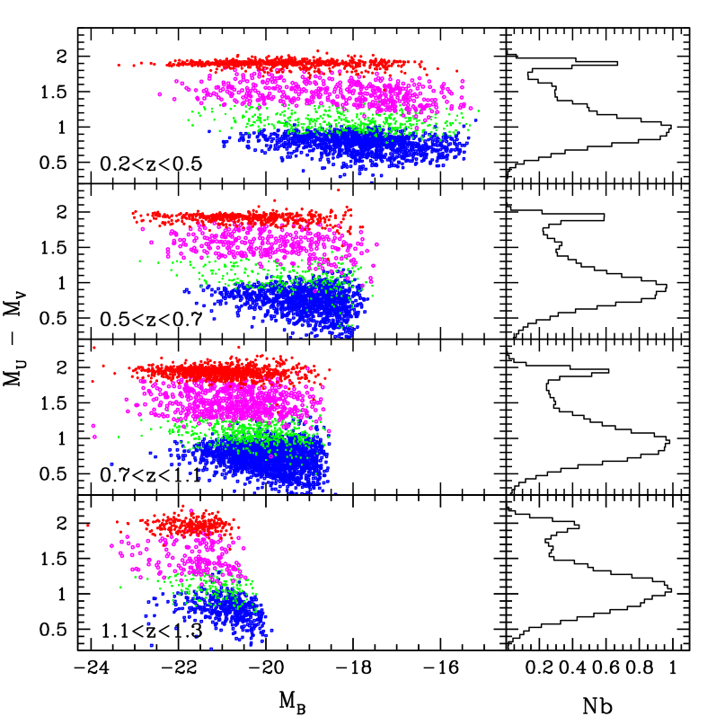
Figure 1: Rest frame $M_{U}-M_{V}$ colour as a function of B-band absolute magnitude for the D1 field. Each panel from top to bottom corresponds to the redshift bins used in this paper. The points show the four different best-fitting spectral types. In the colour version of this figure (available electronically) red, magnenta, green and blue points correspond to Coleman et al. Ell, Sbc, Scd, and Irr templates. The right-hand panels show the colour distribution for each redshift slice.

Galaxies have been classified using multi-colour information in a similar fashion to other works in the literature (for example Lin et al., 1999; Wolf et al., 2003; Zucca et al., 2006). For each galaxy the rest-frame colours were matched with four templates from Coleman et al. (1980) (hereafter referred to “Coleman, Wu and Weedman” or “CWW” templates). These four templates have been optimised using the VVDS spectroscopic redshifts, as described in Ilbert et al., and are presented in Fig.2 of this work. Galaxies have been divided in four types, corresponding to the optimised E/S0 template (type one), early spiral template (type two), late spiral template (type three) and irregular template (type four). Type four includes also starburst galaxies. Note that, in order to avoid introducing dependencies on any particular model of galaxy evolution, we did not apply templates corrections aimed at accounting for colour evolution as a function of redshift.

We show in Figure 1 the rest-frame colour distribution of the galaxies for each type. Type one galaxies comprise most of the galaxies of the red peak of the bimodal colour distribution. The other types are distributed in the blue peak. Galaxies become smoothly bluer from type one to type four respectively.

3 Measuring galaxy clustering

3.1 Introduction

There are two principal approaches which may be used to measure the clustering of objects with photometric redshifts. One is simply to isolate galaxies in a certain redshift range using photometric redshifts, and then to compute the projected correlation function $w(\theta)$ for galaxies in this slice, as has long been done for magnitude-limited samples. However, the additional information provided by photometric redshifts on the bulk properties of our slice (its redshift distribution) allows us to use the Limber’s equation (Limber, 1953) to invert the projected correlation function and recover spatial correlations at the effective redshift of the slice. These computations are easy to perform and are relatively insensitive to systematic errors in the photometric redshifts as one just integrates over all galaxies in a given redshift slice; it has already been used extensively in smaller surveys and is usually the method of choice when only small numbers of galaxies or poorer-quality photometric redshifts are available, and has been used extensively over the past few years (see, for example Daddi et al. (2001) or Arnouts et al. (1999)). It has the disadvantage that it provides only limited information on the shape of the angular correlation function as one measures a correlation function integrated over a given redshift slice.

A second approach is to decompose the redshift of each galaxy into it’s components perpendicular($r_{p}$) and parallel ($\pi$) to the observer’s line of sight, and then to compute a full two-dimensional correlation function $\xi(r_{p},\pi)$ based on pair counts of galaxies in both directions. Finally, one computes the sum of this clustering amplitude in the direction parallel to the line of sight, $w_{p}$. In spectroscopic surveys, this has the advantage of removing the effect of redshift-space distortions caused by infall onto bound structures. This technique has been used successfully for many spectroscopic redshift surveys (Davis & Peebles, 1983; Le Fèvre et al., 1996; Zehavi et al., 2005) and some attempts have been made to apply it to samples with lower-accuracy photometric redshifts (Phleps et al., 2006). It has the advantage that it can provide direct information on the shape of the correlation function but this comes at the price of much greater sensitivity to systematic errors in the photometric redshifts (for example, integration over a much larger range in redshift space is necessary). We plan an analysis using this technique in a forthcoming article, but in this paper we adopt a conservative approach, as we are primarily interested in the overall clustering properties of our galaxy samples.

3.2 Projected angular clustering

We first use our photometric redshift catalogue to produce a galaxy sample generated using a given selection criterion, for example either by absolute or apparent magnitude, redshift or type. This same selection criterion is applied to catalogues for all four fields.

From these masked catalogues of object positions, we measure $w(\theta)$, the projected angular correlation function, using the standard Landy & Szalay (1993) estimator:

$$w(\theta)={\mbox{DD}-2\mbox{DR}+\mbox{RR}\over\mbox{RR}}$$ (1)

where $DD$, $DR$ and $RR$ are the number of data–data, data–random and random–random pairs with separations between $\theta$ and $\theta+\delta\theta$. These pair counts are appropriately normalised; we typically generate random catalogues with ten times higher numbers of random points than input galaxies.

An important point to consider is that, of course, the precision of our photometric redshifts are limited. In a given redshift interval, $z_{1}<z<z_{2}$ it is certainly possible that a given galaxy may be in fact outside this range. To account for this, we employ a weighted estimator of $w(\theta)$, as suggested by Arnouts et al. (2002). In this scheme we weight each galaxy by the fraction of the galaxy’s probability distribution function enclosed by the interval $z_{1}<z<z_{2}$.

In this case for each pair we must now compute

$$DD=\sum_{i,j}^{N}{P^{i}}{P^{j}};DR=\sum_{i,j}^{N_{d},N_{r}}{P^{i}}$$ (2)

where $P^{i,j}$ is the integral of object’s probability distribution function in the redshift interval $z_{1}<z<z_{2}$. The total ’effective’ number of galaxies becomes

$$N_{\rm eff}=\sum_{i=1}^{i=N_{gal}}P^{i}$$ (3)

We may then fit $w(\theta)=A_{w}\theta^{-\delta}$ to find the best-fitting amplitudes and slopes $A_{w}$ and $\delta$, after first correcting for the “integral constraint” which arises because the mean density is estimated by the survey itself,

$$C={1\over{\Omega^{2}}}\int\int\omega(\theta)d\Omega_{1}d\Omega_{2}$$ (4)

where $\Omega$ is the total area subtended by our survey. We compute C by numerical integration of Equation (4), discounting pairs closer than 1”, corresponding to the resolution limit of our data. The integral constraint correction is subtracted from the power law. We always fit our data on scales where theintegral constraint correction is negligible.

We compute $w$ in a series of logarithmically spaced bins from $\log(\theta)=-3$ to $\log(\theta)=-0.2$ with $\delta\log(\theta)=0.2$, where $\theta$ is in degrees. In the following sections we will consider both measurements derived from each field separately (using that field’s redshift distribution) and also measurements constructed from the sum of pairs over all fields (in which case we use a combined, weighted redshift distribution derived from all fields).

3.3 Derivation of spatial quantities

We can associate each value of $A_{w}$ and $\delta$ with a corresponding comoving correlation length, $r_{0}$ by making use of the relativistic Limber equation (Peebles, 1980). For further discussion of this method see, for example Daddi et al. (2001) or Arnouts et al. (1999). If we assume that the spatial correlation function can be expressed as $\xi(r)=(r/r_{0})^{-\gamma}$ (where $\gamma=1-\delta$ and $\Gamma$ is the incomplete Gamma function)

$$w(\theta)={\sqrt{\pi}\Gamma((\gamma-1)/2)\over{\Gamma(\gamma/2)}}{\int g(z)(dN/dz)^{2}r_{0}(z)^{\gamma}dz\over[\int(dN/dz)dz]^{2}}\theta^{1-\gamma}$$ (5)

where $dN/dz$ represents the redshift distribution and $\theta$ is the angular separation on the sky. Here g(z) depends only on cosmology and is given by:

$$g(z)=(dx/dz)^{-1}x^{1-\gamma}F(x)$$ (6)

with the metric defining $x$ and $F(x)$:

$$ds^{2}=c^{2}dt^{2}-a^{2}[dx/F(x)^{2}+x^{2}(\sin^{2}\theta d\phi^{2})]$$ (7)

Defining

$$r_{0}^{\gamma}(z_{\rm eff})={\int^{z_{2}}_{z_{1}}g(z)(dN/dz)^{2}r_{0}(z)^{\gamma}dz\over\int_{z_{1}}^{z_{2}}g(z)(dN/dz)^{2}dz}$$ (8)

and assuming that the correlation amplitude is constant over our redshift interval $z_{1}<z<z_{2}$ and that $w(\theta)=A_{w}\theta^{1-\gamma}$ we can write:

$$A_{w}=r_{0}^{\gamma}(z_{\rm eff})\sqrt{\pi}{\Gamma((\gamma-1)/2)\over{\Gamma(\gamma/2)}}{\int^{z_{2}}_{z_{1}}g(z)(dN/dz)^{2}dz\over[\int_{z_{1}}^{z_{2}}(dN/dz)dz]^{2}}$$ (9)

Thus, given a measurement $A_{w}$ of the correlation function amplitude for the redshift slice under consideration and a knowledge of that slice’s redshift distribution we can derive $r_{0}(z_{\rm eff})$.

Given that we have four separate fields, we may derive $r_{0}$ from a “global” $w(\theta)$ derived from the sum of pairs over all fields and computed using the average, weighted $dn/dz$. Alternatively, we can compute $r_{0}$ for each field using that field’s redshift distribution and individual correlation function amplitudes; the final value of $r_{0}$ is then calculated simply as the average over all four fields. We find that, in general, these methods agree for most samples. However, in some cases the error bars are larger with the field-to-field measurements. This is discussed in more detail in the following section.

3.4 Error estimates on $w(\theta)$

We have investigated two different approaches to estimate the errors on our measurements of $r_{0}$. As described above, for each of our four fields, we compute $r_{0}$ from a fit to a measurement of $w(\theta)$ and the redshift distribution for that field. We then compute the variance in $r_{0}$ and $\gamma$ over all fields.

In the second method, for each sample, we compute the sum of the pairs over all fields at each angular bin. The error bar at each angular bin is then calculated from the variance in $w(\theta)$ over all fields. If $w_{av}$ is the mean correlation function then $w_{i}$ is the correlation function for each field, then the error over the $n$ fields of the CFHTLS is given as

$$\sigma^{2}={1\over(n-1)}{\sum_{i=1}^{n}(w_{av}-w_{i})^{2}}$$ (10)

where $n=4$ for the CFHTLS (note that $w_{av}$ is only used in this computation and not in any other part of the analysis).

A “global” correlation length is determined using the average redshift distribution over four fields. In this case, the error in $r_{0}$ is computed from the error in the best fitting $A_{w}$. This error is, in turn, computed from the covariance matrix derived using the Levenberg-Marquardt non-linear fitting routine, as presented in Numerical Recipes Press et al. (1986).

We find that in most cases the error bars in $r_{0}$ estimated by these two different methods are consistent. However at lower redshifts ranges ($0.2<z<0.6$), where the numbers of galaxies is smaller, field-to-field dispersion is higher than the global errors. Further investigations reveal this is due to the presence of a single field (d2) which has anomalously higher correlation lengths. Properties of this field are discussed in detail in McCracken et al. (2007). This is undoubtedly due to the presence of very large structures at $z\sim 0.3$ and $z\sim 0.7$ in this field We believe that our ’global’ correlation function provides a more robust estimate of the total error and we adopt this measurement for the remainder of the paper.

4 Results

4.1 Magnitude limited samples

Figure 2: The amplitude of the angular correlation $w$ as a function of angular separation $\theta$ (in degrees) for $17.5<i^{\prime}<24$ galaxies selected in the four deep fields of the CFHTLS in a range of redshift slices. The error bars correspond to the amplitude of the field-to-field variance over all fields. The dashed line shows the best-fitting power law correlation function after the subtraction of the appropriate integral constraint.

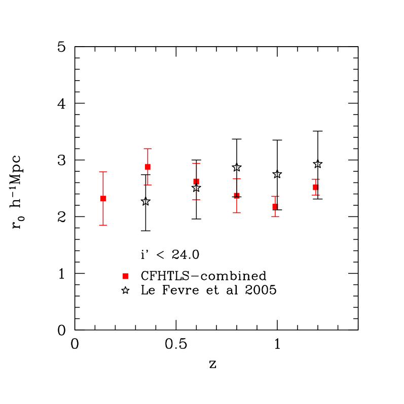
Figure 3: The comoving correlation length, $r_{0}$ as a function of redshift for the four combined CFHTLS fields (filled squares) compared to literature values (open symbols) computed for a galaxy sample limited at $i^{\prime}<24.0$. For these fits, both $\gamma$ and $r_{0}$ are free parameters. The error bars on these fits are computed from the field-to-field variance in each bin in $w$, as described in Section 3.

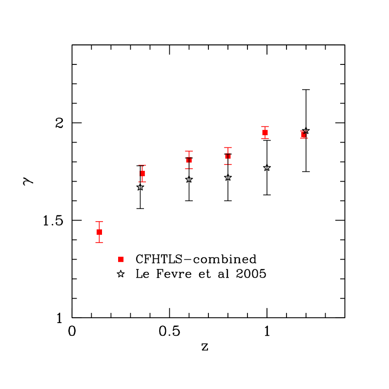
Figure 4: The best-fitting slope $\gamma$, as a function of sample median redshift for the four CFHTLS fields combined (filled squares) compared to literature measurements (open symbols) for a sample selected with $17.5<i^{\prime}<24.0$ at each redshift slice.

Can photometric redshifts be used to make reliable measurements of galaxy clustering at $z\sim 1$? In this Section we will construct a sample similar to those already in the literature in order to address this question. We consider galaxies selected by redshift and apparent magnitude. In each field we divide our catalogues into a series of bins of width $\delta z=0.2$ over the range $0.2<z<1.2$. In each bin, galaxies with $17.5<i_{AB}<24.0$ are selected to match the criterion used by the VIMOS-VLT deep survey (VVDS) as presented in Le Fèvre et al. (2005a) (we note that the Megacam instrumental $i^{\prime}$ magnitudes are very close to the CFH12K instrumental $I$ magnitudes used in Le Fèvre et al.). Following the procedures outlined in Section 3, we measure the weighted pair counts at each angular separation for each field and sum them together. Equation (1) is used to derive a “global” $w(\theta)$. The error bar at each bin of angular separation is computed from the variance of the individual measurements of $w(\theta)$ over all four fields, as described in Equation (10). These results are illustrated in Figure 2, which shows the amplitude of $w$ for all four fields for a range of redshift slices. We note that in all redshift slices except the lowest-redshift one, at intermediate scales, $w(\theta)$ is well represented by a power law. In addition our error bars are reassuringly small. This global $w(\theta)$ is then fitted with the usual power law, correcting for an integral constraint corresponding to a total area of $3.2\deg^{2}$.

In calculating the correlation amplitude $r_{0}$ at the effective redshift of each slice we use a redshift distribution derived from the weighted, summed $dn/dz$ from each field. Our results are displayed in Figures 3 and 4. They are consistent with the measurements from the VVDS deep survey (open symbols; Le Fèvre et al., 2005a), which was based on a much smaller sample of $\sim 7000$ spectroscopic redshifts. Our data does show some evidence for a decline in the correlation amplitude strength in the interval $0.5<z<1.1$, as well as a slightly higher slope, in contrast with this earlier work. This effect will be discussed in more detail in Section 5.

4.2 Luminosity dependent clustering at $z\sim 0.5$ and $z\sim 1.0$

The main difficulty in interpreting Figures 3 and 4 is that at each redshift slice the sample’s median absolute luminosity changes significantly as a consequence of the selection in apparent magnitude. This is evident if one considers Figure 5 which shows a two-dimensional image of the objects distribution in the absolute magnitude-redshift plane. Slices extracted at lower redshift are dominated by galaxies of intrinsically low absolute luminosity.

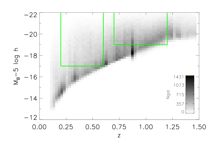
Figure 5: Gray-scaled histogram showing the distribution of galaxies as a function of absolute magnitude and redshift for four CFHTLS fields for all galaxy types and for an apparent magnitude limit of $i^{\prime}<24.5$.

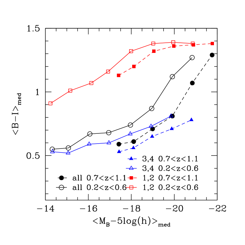
Figure 6: Median rest-frame (B-I) colour versus median rest frame $B-$band absolute luminosity for samples at $0.2<z<0.6$ (open symbols, solid lines) and $0.7<z<1.1$ (filled symbols, dotted lines). For each redshift range we show all galaxy types (circles), types one and two (squares) and types three and four (triangles).

To investigate the dependence of galaxy clustering amplitude on absolute luminosity, in this Section we extract samples in two fixed redshift intervals selected from the absolute-magnitude/luminosity plane. We consider galaxies between $0.2<z<0.6$ and $0.7<z<1.1$. In each redshift range we select a minimum absolute magnitude (shown by the solid lines in Figure 5) so that the median redshift of galaxies selected in each slice of absolute luminosity is approximately constant. At each redshift interval we separate the galaxy population into “early” (types one and two) and “late” (types three and four). We also consider samples comprising all galaxy types. These samples are illustrated in Figure 6, where the median rest-frame Johnson $(B-I)$ colour is plotted as a function of median rest-frame $M_{B}$ magnitude. In both high- and low- redshift slices, changes in the absolute magnitude bin produces the largest changes in rest-frame colours. It is also clear that galaxy populations become progressively bluer at higher redshifts (dotted lines and filled symbols), at the same bin in absolute magnitude.

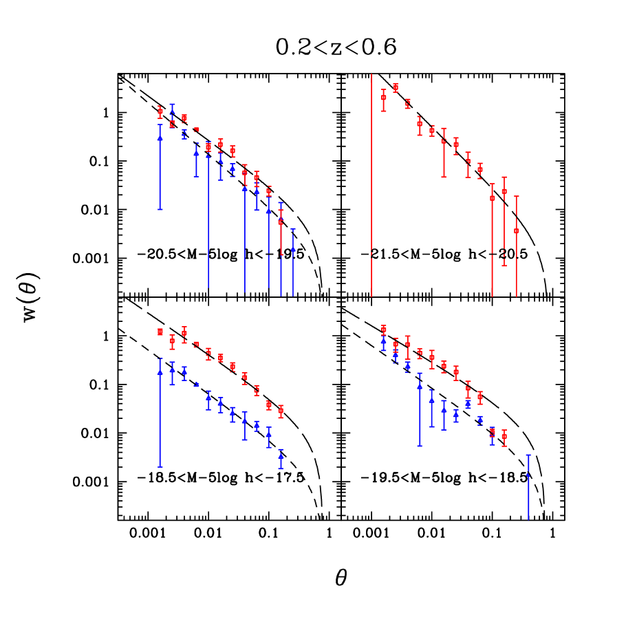
Figure 7: The amplitude of the angular correlation $w$ as a function of angular separation $\theta$ (in degrees) for $i^{\prime}<24.5$ galaxies in the redshift range $0.2<z<0.6$. Each panel shows galaxies selected in a different, independent, slice in absolute luminosity. Squares represent the early-type population (types 1 and 2) whereas triangles show the late-type population. The dashed and long-dashed lines shows the adopted best-fit. The error bars at each angular separation correspond to field-to-field variance measured over the four survey fields.

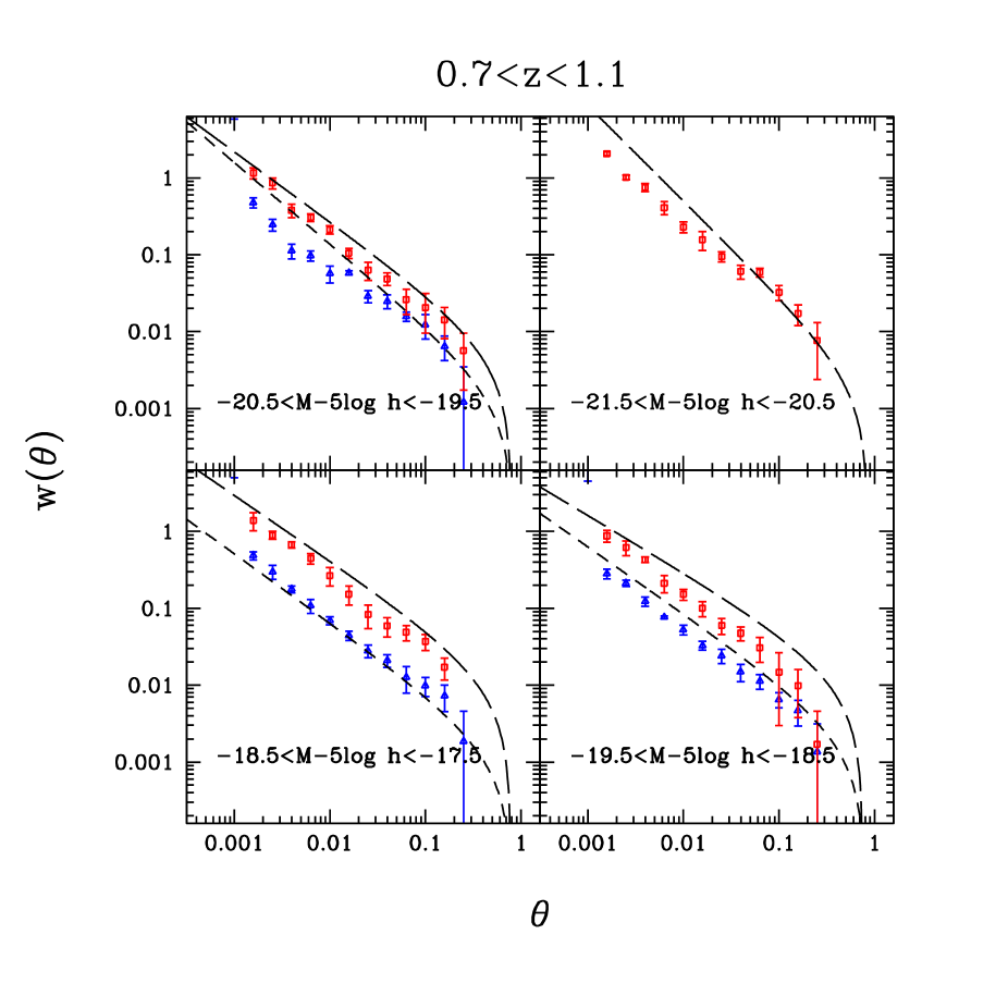
Figure 8: Similar to Figure 7: the amplitude of the angular correlation $w$ as a function of angular separation $\theta$ (in degrees) for red and blue $i^{\prime}<24.5$ galaxies in the redshift range $0.7<z<1.1$. The dashed and long-dashed lines shows the adopted best-fit for the same bin in absolute luminosity in the lower redshift range $0.2<z<0.6$. The error bars at each angular separation correspond to field-to-field variance measured over the four survey fields.

Our type-selected correlation functions for galaxies in the redshift range $0.2<z<0.6$ are displayed in Figure 7, and for the higher redshift range in Figure 8. These plots show the amplitude of the angular correlation function $w$ as a function of angular separation, $\theta$, for different slices of absolute magnitude. In each panel we show correlation functions measured for the red and blue (early and late) populations. The size of the error bars at each angular separation corresponds to the amplitude of the field-to-field cosmic variance computed over the four fields. The long-dashed and dashed lines show the fitted amplitudes for the red and blue populations respectively. For the higher redshift bin, we superimpose the fitted amplitudes at the same bin in absolute luminosity at the lower redshift interval. At all redshifts and absolute luminosity ranges, galaxies with redder rest-frame colours are more clustered than their bluer counterparts.

Because of the strong covariance between $\gamma$ and $r_{0}$ it is useful to consider contours of constant $\chi^{2}$ at each slice in absolute magnitude. This is shown in Figure 9. The vertical and horizontal lines mark an arbitrary reference point. Solid lines indicate galaxies with $0.2<z<0.6$ and dotted lines those with $0.7<z<1.1$. From these plots we see a gradual increase in comoving correlation length as a function of absolute rest-frame luminosity. We also see some evidence for a slight decrease in the comoving correlation length at given fixed absolute luminosity between higher and lower redshift slices.

Figures 10 and 11 show the comoving correlation function $\chi^{2}$ contours for red and blue populations in both redshift ranges; and correspond to the angular correlation functions presented in Figures 7 and Figures 8. Figure 9 shows the comoving correlation length for the full galaxy population in both redshift ranges.

The results presented in this Section are summarised in Figures 12, 13 and in Tables 1 and 2. These figures show the best-fitting correlation amplitude as a function of absolute luminosity for the three different samples (early, late and the full galaxy population) in the two redshift ranges ($0.2<z<0.6$ and $0.7<z<1.1$) considered in this Section.

Considering these plots, several features are apparent. Firstly, at all absolute magnitude slices and in both redshift ranges, early-type galaxies are always more strongly clustered (higher values of $r_{0}$) than late-type galaxies. Secondly, we note that clustering amplitude for the late-type population is remarkably constant, remaining fixed at $\sim 2h^{-1}$ Mpc over a large range of absolute magnitudes and redshifts. The behaviour of the early-type population is more complicated. For the $0.2<z<0.6$ bin, we some evidence that as the median luminosity increases, the clustering amplitude of this population decreases, from around $\sim 6h^{-1}$ Mpc for the faintest bins, to $\sim 5h^{-1}$ Mpc. We note that the difference in clustering amplitude between the early and late populations is smaller for the higher-redshift bin. We also note that the clustering amplitudes we derive for our blue and full-field galaxy populations are considerably lower than those reported by Norberg et al. (2002) at lower redshifts.

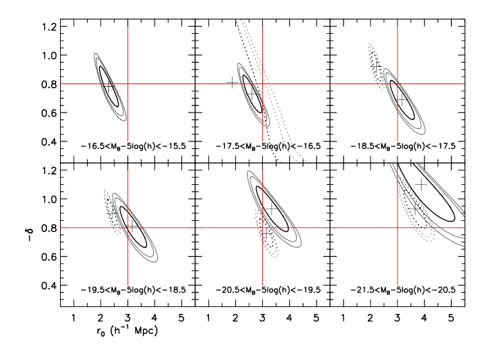
Figure 9: The comoving correlation length $r_{0}$ and slope $\delta=1-\gamma$ as a function of median absolute luminosity and redshift for low-redshift ($0.2<z<0.6$; solid lines) and high redshift ($0.7<z<1.1$; dotted lines) populations for four fields of the CFHTLS-deep. Each panel shows contours of constant chi-squared values for $1,2,$ and $3\sigma$ confidence levels with the plus symbol marking the minimum chi-squared value. For convenience, lines of constant slope and comoving correlation length are plotted.

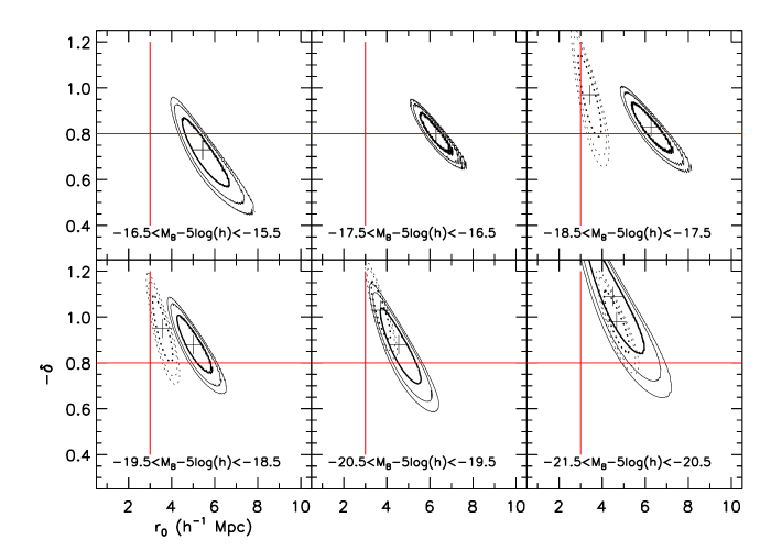
Figure 10: The comoving correlation length $r_{0}$ and slope $\delta=1-\gamma$ as a functions of absolute luminosity and redshift for early-type galaxies for the four fields of the CFHTLS. Each panel shows contours of constant chi-squared values for $1$,$2$, and $3\sigma$ confidence levels with the plus symbol marking the minimum. The solid and dotted lines shows galaxies in the redshift bin $0.2<z<0.6$ and $0.7<z<1.1$ respectively for the same range of absolute luminosities. We note that in the $-18.5<M_{B}-5\log(h)<-17.5$ and $-19.5<M_{B}-5\log(h)<-18.5$ luminosity ranges the clustering amplitude of early type galaxies at different redshifts are well separated.

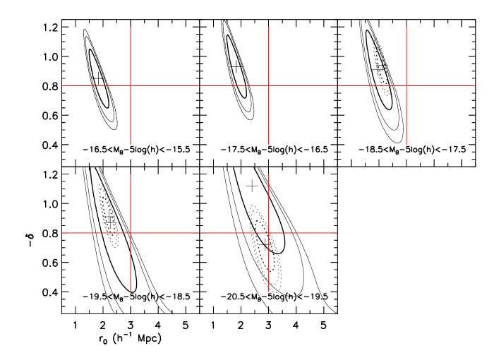
Figure 11: The comoving correlation length $r_{0}$ and slope $\delta=1-\gamma$ as a function of absolute luminosity and redshift for late-type populations for the four fields of the CFHTLS. Each panel shows contours of constant chi-squared values for $1$,$2$, and $3\sigma$ confidence levels with the plus symbol marking the minimum. The solid and dotted lines shows galaxies in the redshift bin $0.2<z<0.6$ and $0.7<z<1.1$ respectively for the same range of absolute luminosities.

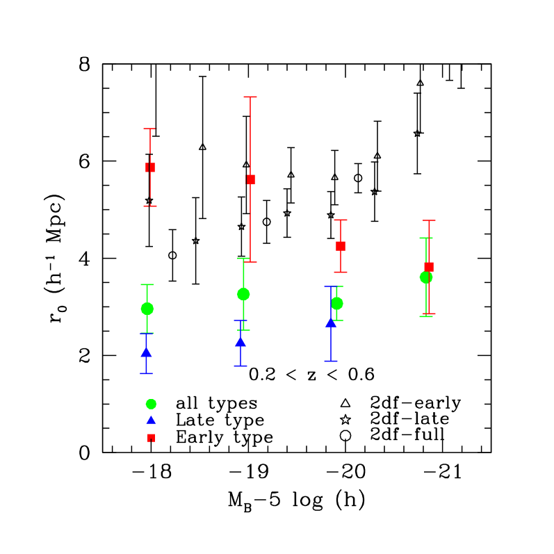
Figure 12: The comoving correlation length $r_{0}$ as a function of median absolute luminosity and type for objects in the redshift range $0.2<z<0.6$. Filled circles show the full galaxy population. In addition to type selection, the galaxy sample is selected in one-magnitude bins of absolute luminosity. Triangles and squares represent the late and early-type populations respectively.

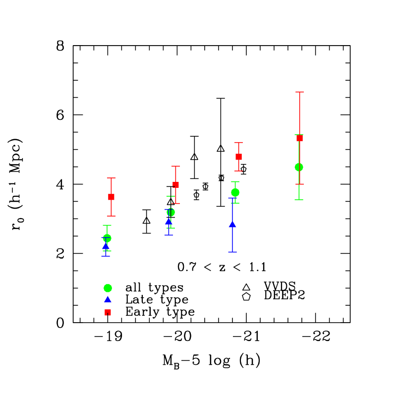
Figure 13: Similar to Figure 12; here we show measurements from our $0.6<z<1.1$ sample. Points from the literature from the measurements made by the DEEP2 and VVDS surveys.

We carried out several test to verify the robustness of the higher correlation amplitudes observed for the fainter red galaxy population at $z\sim 0.5$. Selecting galaxies with redder rest-frame colours (classified as type one) in larger bins of absolute magnitude we also measure higher clustering amplitudes for objects fainter than $M_{B}-5\log h\sim-19$. We also note that the origin of the large error bar for the bin at $M_{B}-5\log h=-19$ is due to the presence of structures in one of the four fields; interestingly, for the D1 field, for this faint red population, the correlation function does not follow a normal power-law shape. Our resulting error bars reflect this behaviour, but it is clear that for certain galaxy populations, for instance the bright elliptical population, simple power-law fits are not appropriate.

In the redshift range $0.7<z<1.1$ we have compared our measurements of pure luminosity dependent clustering (i.e., without type selection) to works in the literature computed using smaller samples of spectroscopic redshifts, namely Pollo et al. (2006) and Coil et al. (2006), shown in Figure 13 as the open triangles and open stars respectively. Their points should be compared with the full circles derived from our measurements. In general the agreement is acceptable, although for higher luminosity bins, our amplitudes are below the measurements from the DEEP2 survey (although it seems that the amplitude of their error bars is perhaps underestimated).

For all the plots previously shown in this Section we fitted simultaneously for the slope and amplitude of the galaxy correlation function. In Figure 14 and Figure 15 we summarise our results from our low and high redshift samples. Figure 15 shows the slope $1-\gamma$ as a function of absolute luminosity for early-type, late type, and full-field populations at high redshifts. Figure 14 presents the results from the $0.2<z<0.6$ sample. Error bars are computed from the field-to-field variance.

Interestingly, we find for the higher redshift bin ($0.7<z<1.1$) the slope is relatively insensitive to absolute magnitude. However, at lower redshifts, luminous red galaxies have a steeper correlation function slope than fainter galaxies. A similar effect is observed in the SDSS and two-degree field surveys at lower redshifts (Norberg et al., 2002).

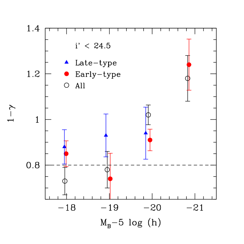
Figure 14: Best-fitting slope $1-\gamma$ of $w$ as a function of median absolute luminosity at $0.2<z<0.6$ for the early-type population (filled circles), late-type population (triangles) and full population (open circles). Slopes are plotted as a function of the median absolute magnitude in each slice of one magnitude in width.

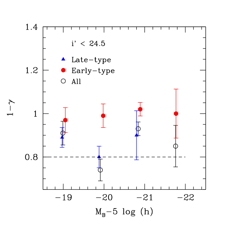
Figure 15: As in Figure 12 but for the redshift range $0.7<z<1.1$. Slopes are plotted as a function of the median absolute magnitude in each bin of one magnitude in width.

$\langle M_{B}\rangle$	$N_{\rm gals}$	$\langle B-I\rangle$	$z_{\rm eff}$	$r_{0}$	$\delta$
All
-18.0	15741	0.74	0.46	$3.0\pm 0.5$	$0.7\pm 0.06$
-18.9	11025	0.87	0.46	$3.2\pm 0.3$	$0.9\pm 0.06$
-19.9	6607	1.12	0.45	$3.1\pm 0.3$	$1.0\pm 0.04$
-20.8	2153	1.27	0.46	$3.6\pm 0.8$	$1.2\pm 0.10$
Red
-18.0	3704	1.32	0.42	$5.9\pm 0.8$	$0.8\pm 0.06$
-19.0	3957	1.38	0.43	$5.6\pm 1.7$	$0.7\pm 0.11$
-19.9	3656	1.39	0.44	$4.2\pm 0.5$	$0.9\pm 0.05$
-20.9	1567	1.38	0.45	$3.8\pm 1.0$	$1.2\pm 0.11$
Blue
-17.9	12037	0.67	0.47	$2.0\pm 0.4$	$0.9\pm 0.07$
-18.9	7068	0.73	0.47	$2.2\pm 0.5$	$0.9\pm 0.09$
-19.9	2951	0.81	0.47	$2.6\pm 0.8$	$0.9\pm 0.11$

Table 1: Low redshift sample ($0.2<z<0.6$). Columns show the median rest-frame $B-$band absolute luminosity, total number of galaxies over the four fields, median absolute rest-frame B-I colour, effective redshift, best fitting correlation length and slope.

$\langle M_{B}\rangle$	$N_{gals}$	$\langle B-I\rangle$	$z_{\rm eff}$	$r_{0}$	$\delta$
All
-19.0	40483	0.71	0.90	$2.4\pm 0.4$	$0.9\pm 0.05$
-19.9	25452	0.81	0.91	$3.2\pm 0.5$	$0.7\pm 0.05$
-20.8	9689	1.07	0.91	$3.8\pm 0.3$	$0.9\pm 0.03$
-21.8	1664	1.29	0.93	$4.5\pm 0.9$	$0.8\pm 0.10$
Red
-19.1	8639	1.32	0.88	$3.6\pm 0.6$	$1.0\pm 0.06$
-20.0	8859	1.36	0.90	$4.0\pm 0.5$	$1.0\pm 0.05$
-20.9	5511	1.37	0.91	$4.8\pm 0.4$	$1.0\pm 0.03$
-21.8	1280	1.38	0.93	$5.3\pm 1.3$	$1.0\pm 0.11$
Blue
-19.0	31844	0.65	0.91	$2.2\pm 0.3$	$0.9\pm 0.05$
-19.9	16593	0.71	0.91	$2.9\pm 0.4$	$0.8\pm 0.05$
-20.8	4178	0.78	0.91	$2.8\pm 0.8$	$0.9\pm 0.11$

Table 2: High redshift sample ($0.7<z<1.1$). Columns show the median rest-frame $B-$band absolute luminosity, total number of galaxies over the four fields, median absolute rest-frame B-I colour, effective redshift, best fitting correlation length and slope.

4.3 Clustering of bright early type galaxies

In Figure 16 we plot the clustering amplitudes of bright early-type galaxies in our survey; filled squares indicate galaxies of types one and two, and open squares represent a pure type one sample. As expected, the clustering amplitudes of the pure type one population (with overall redder rest-frame colours) are higher than the combined type one and two samples. (We have also measured the clustering amplitude of the pure type four population and find that in this case clustering amplitudes are lower than the combined sample of types three and four.) Error bars are computed from the field-to-field variance.

Several authors have presented clustering measurements as a function of either absolute luminosity, type or redshift. For example, Meneux et al. (2006) described measurements in the VVDS spectroscopic redshift survey of the projected correlation function for early- and late-type galaxies. Their galaxies are classified in the same way as in this paper, using CWW templates. However, in their sample galaxies were selected by apparent magnitude; at $z\sim 1$, their rest frame luminosities are comparable to the brightest galaxies in our sample. We compare these $z\sim 1$ with our data; they are shown as the open circles in Figure 16. Finally, the open triangles represent measurements from Brown et al. (2003) who measured clustering of red galaxies selected using three-band photometric redshifts in the NOAO wide survey. Their results are above ours by at least one or two standard deviations. In general we note that our results are lower than literature measurements and speculate that this could be the consequence of a slight loss of signal due our use of photometric redshifts. The broad trend seen in our measurements is that the clustering amplitude of bright early-type galaxies does not change with redshift.

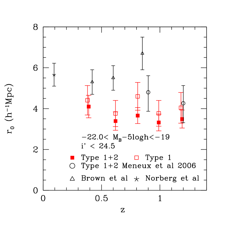
Figure 16: Clustering amplitude of luminous red galaxies. Open and filled squares show measurements for type one and type one and two combined galaxy samples. Other points show measurements from the literature for early type galaxies selected using a variety of methods.

4.4 Redshift-dependent clustering

How does the comoving correlation length of the various galaxy populations investigated here depend on redshift? Over the full range redshift range ($0.2<z<1.1$), as is apparent from Figure 5, this measurement is only possible for the brightest galaxies; at higher redshifts, intrinsically fainter galaxies drop out of our survey. For each of the redshift bins used in Figure 2 we selected galaxies with $-22.0<M_{B}-5\log h<-19$ and measured $r_{0}$ and $\gamma$ as above. The derived amplitudes for this sample are shown as the stars in Figure 17. We also selected at each redshift bin early type galaxies (types 1 and 2) and late type galaxies (types 3 and 4); these are represented by squares and triangles in Figure 17. We find that the median absolute magnitude at each bin is $M_{B}-5\log h\sim-19.6$ for the early types and $M_{B}-5\log h\sim 19.4$ for the late types. The full galaxy population has an absolute magnitude of $M_{B}-5\log h\sim-19.5$. From $0.4<z<1.2$, these values changes by at most 0.1 magnitudes. As in previous plots, the size of the error bars represent cosmic variance errors over the four fields.

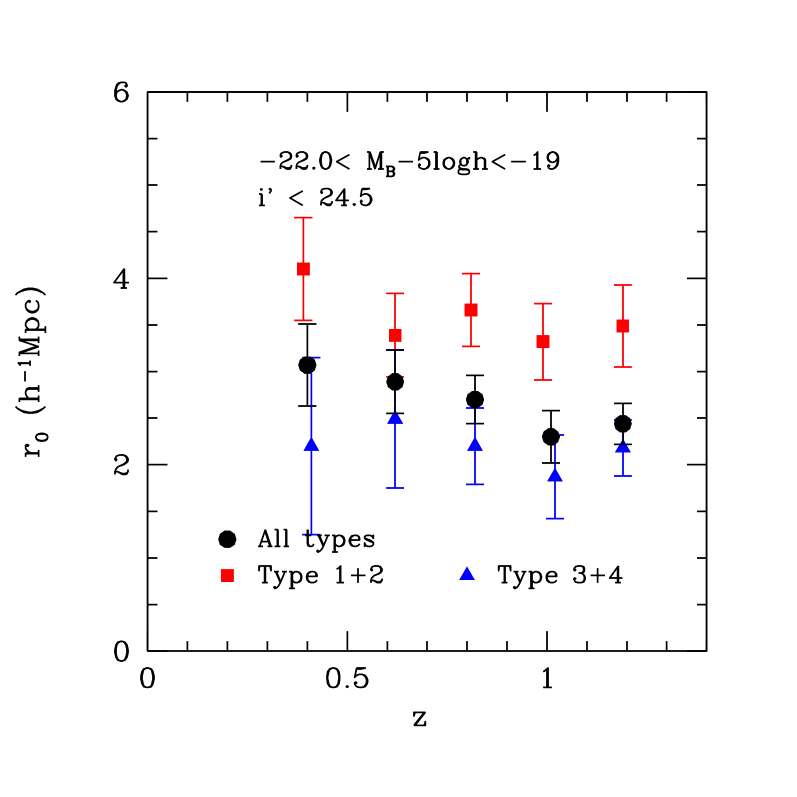
Figure 17: Redshift dependence of comoving galaxy correlation length $r_{0}$ for a series of volume limited samples for early types (squares), late types (triangles) and for the full sample (filled circles).

We find that in the redshift range $0.4<z<1.2$ probed by our survey, early-type galaxies are always more clustered than late type galaxies as we have already found in in the previous Sections. Moreover, the difference in clustering amplitudes between these two populations is approximately constant with redshift. (Note that the galaxy samples examined here correspond to essentially the brightest bins plotted in Figures 12 and Figure 13). We also find that the clustering of the $-22<M_{B}-5\log h<-19$ luminosity-limited full galaxy sample (i.e., without including a type selection) decreases steadily from $z\sim 0.4$ to $z\sim 1.2$.

4.5 Relative bias

We can also compute the relative bias between different galaxy populations at different redshifts. At each redshift range in Section 4.2 ($0.2<z<0.6$ and $0.7<z<1.1$) we compute the relative bias $b$ as follows:

$$b=b_{a}/b_{b}=\sigma_{8}(a)/\sigma_{8}(b)$$ (11)

We adopt the usual definition for $\sigma_{8}$ (Peebles, 1980),

$$\sigma_{8}=\sqrt{(C_{\gamma}(r_{0}/8)^{\gamma}),}$$ (12)

Where is $C\gamma$ is a constant which depends on $\gamma$:

$$C_{\gamma}={72\over(3-\gamma)(4-\gamma)(6-\gamma)2^{\gamma}}$$ (13)

In Figure 18 we plot the relative bias between the early and late-type populations for our low and high redshift samples (open and filled circles respectively) as a function of absolute rest-frame luminosity. Error bars are computed from the field-to-field variance. From our data it is clear that the relative bias between the early and late type populations declines between $z\sim 0.5$ and $z\sim 1$.

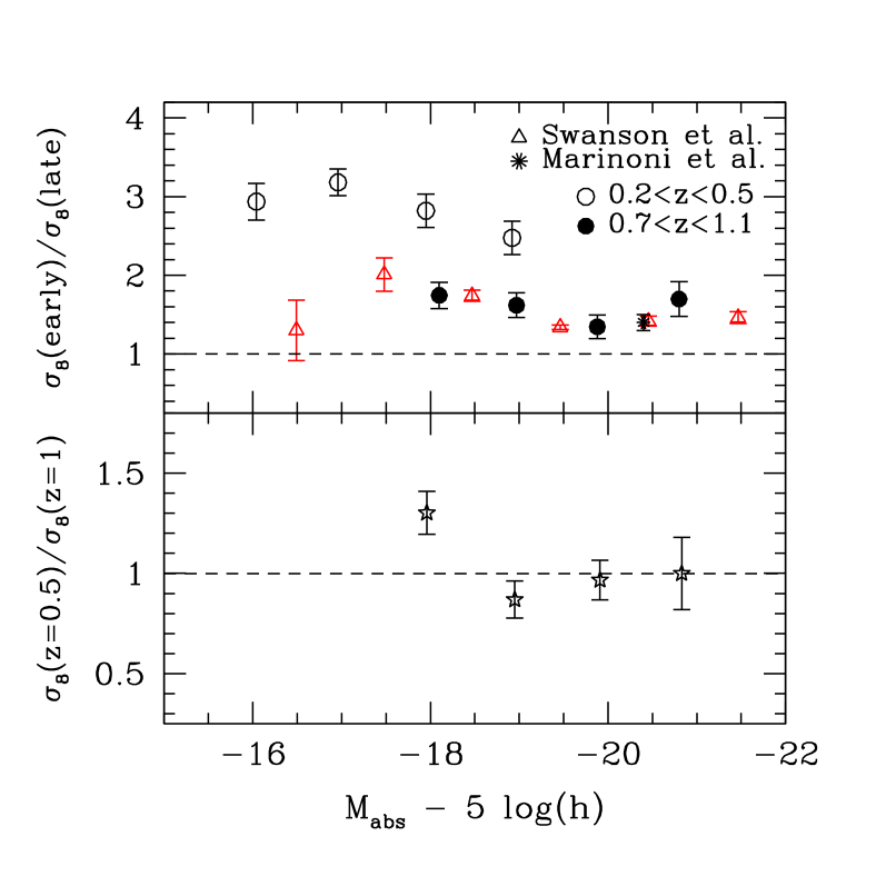
Figure 18: Top panel: relative bias between early and late-type populations at $z\sim 0.5$ (open circles) and $z\sim 1$ (filled circles). The open triangles and star show measurements from Swanson et al. (2007) and Marinoni et al. (2005) respectively. Bottom panel: relative bias between the low- and high-redshift full galaxy sample. For both panels, biases are plotted as a function of the median absolute rest-frame magnitude in slices of one magnitude in width.

We compare our relative bias between blue and red galaxy populations with measurements in the literature. Marinoni et al. (2005) divided their spectroscopic sample into a red one with rest-frame $(B-I)>0.95$ and a bluer one with $(B-I)<0.68$. By measuring the probability distribution function (PDF) of these two populations, they were able to be measure the relative bias of relatively bright ($M_{B}-5\log(h)\sim-21$) galaxies in the interval $0.6<z<1.1$, indicated by the starred point in Figure 18. Recently, Swanson et al. (2007) investigated the relative bias between red and blue spectroscopic galaxy samples in the Sloan Digital Sky Survey as a function of absolute rest-frame red magnitude. Their results are represented in Figure 18 as open triangles (with an approximate offset applied to convert to rest-frame blue magnitudes used in this paper).

From Figure 18 we see that our measurements at $z\sim 1$ agree with Swanson et al. and Marinoni et al.. Swanson et al. findings are similar to ours: they observe an increase in the relative bias between early and late types at fainter magnitudes. However, at $z\sim 0.5$, our relative bias measurements are considerably higher than either measurements $z\sim 0$ or $z\sim 1$.

5 Discussion

In this paper we have used a sample of 100,000 photometric redshifts in the CFHTLS legacy survey deep fields to investigate the dependency of galaxy clustering on rest-frame colour, luminosity and redshift. The first sample we considered comprises a series of magnitude-selected cuts sampling the full galaxy population from $0.2<z<1.2$. We find that the clustering amplitude decreases gradually from $3h^{-1}$ Mpc at $z\sim 0.3$ declining to $2h^{-1}$ at $z\sim 1.0$. The declining correlation amplitude for the full galaxy population at least to $z\sim 1$ indicates that the field galaxy population must be weakly biased, as this trend follows that of the underlying correlation amplitudes of the dark matter.

We next repeated the same experiment (measuring galaxy clustering in narrow redshift bins) and imposed an additional selection by absolute luminosity and rest-frame colour. Selecting galaxies by slices of absolute luminosity the steady decline in comoving correlation length found for samples selected in apparent magnitude is even more pronounced (Figure 17). The luminous field galaxy population, dominated by blue star-forming galaxies at $z\sim 1$, is clearly only weakly biased with respect to the dark matter distribution.

Turning to rest-frame colour-selected samples at all redshift ranges we consistently find that galaxies with redder rest-frame colours are more strongly clustered than those with bluer rest-frame colours (Figure 17). Such an effect has long been observed for galaxies in the local Universe (for example Norberg et al., 2002; Zehavi et al., 2005; Loveday et al., 1999; Guzzo et al., 1997) and at higher redshifts for samples selected by type and luminosity (Meneux et al., 2006; Coil et al., 2006). Numerical simulations find a similar effect: For example, Weinberg et al. (2004) show that older, redder galaxies are more strongly clustered. This is a generic prediction from most semi-analytic models and hydrodynamic simulations of galaxy formation: older, more massive galaxies formed in regions which collapsed early in the history of the Universe. At the present day such regions are biased with respect to the dark matter distribution.

For the brightest ellipticals ($-22<M_{B}-5\log h<-19$) in our survey, we find that their clustering amplitude does not change with redshift (Figure 17), indicating that at $z\sim 1$ the elliptical population must be strongly biased with respect to the underlying dark matter distribution. Comparing our measurements for objects with redder rest-frame colours with those of other surveys, we find similar clustering amplitudes. Reassuringly, as we demonstrated in Section 4.3 sub-samples of galaxies with redder rest-frame colours produce even higher correlation amplitudes (Figure 16).

In a second set of selections we considered the dependence of galaxy clustering on luminosity and type in two broad redshift bins: $0.2<z<0.6$ and $0.7<z<1.1$ (we leave a ’gap’ in the range $0.6<z<0.7$ to ensure that there is no contamination between high and low redshift ranges). Once again, for the most luminous objects ($M_{B}-5\log h\sim-20$) the correlation amplitude is approximately constant between these two redshift bins. However, for fainter red objects, at a fixed absolute luminosity, we see a decline in correlation amplitude between $z\sim 0.4$ and $z\sim 1$; the same is true for samples selected purely by absolute magnitude. We find no evidence for a change in clustering amplitude at the same luminosity for the blue population with redshift.

At $0.2<z<0.6$, where we are complete to $M_{B}-5\log h\leavevmode\nobreak\ <-17$, we find that red galaxies with $M_{B}-5\log h\sim-20$ are more strongly clustered than bluer galaxies of the same luminosity. Moreover as the sample rest frame luminosity decreases to $M_{B}-5\log h-18$ the clustering amplitude rises from $\sim 4h^{-1}$ Mpc to $\sim 6h^{-1}$ Mpc. A similar effect has been reported in larger, low-redshift samples in the local universe (Swanson et al., 2007; Norberg et al., 2002), where both the Sloan and 2dF surveys have found higher clustering amplitudes for redder objects fainter than $L^{*}$. Some evidence for this effect has also been reported in numerical simulations (Croton et al., 2007), which indicate that this behaviour arises because faint red objects exist primarily as satellite galaxies in halos of massive, strongly clustered red galaxies. This means that less luminous, redder objects reside primarily in higher density environments at $z\sim 0.5$. This is in agreement with recent studies of galaxy clusters at intermediate redshift which indicate a rapid build-up of low luminosity red galaxies in clusters since $z\sim 1$ van der Wel et al. (2007). Our survey is not deep enough to probe to equivalent luminosities at $z\sim 1$.

Conversely for the redshift bin at $0.7<z<1.1$ we see that for the full galaxy population more luminous objects are more strongly clustered: $\sim 2h^{-1}$ Mpc for galaxies with $M_{B}-5\log h\sim-19$ and $\sim 4h^{-1}$ Mpc for galaxies with $M_{B}-5\log h\sim-21$. At all luminosity bins, galaxies with redder rest-frame colours are always more strongly clustered than bluer galaxies.

In both redshift ranges, we measured the slopes of the correlation function as a function of redshift, luminosity and rest-frame colour. At $z\sim 1$ we observe that redder galaxies have steeper slopes; at lower redshifts however different galaxy populations have identical slopes. At these redshifts, we find steeper slopes in our most luminous bin; at higher redshifts, no such obvious trend is apparent (in contrast with Pollo et al. (2006), who saw a clear dependence of slope on absolute luminosity).

We have also computed the relative bias between red and blue galaxies at $z\sim 1$ and $z\sim 0.5$. At $z\sim 1$ our results agree with measurements in the literature. Our measurements at $z\sim 0.5$ are significantly above measurements made at $z\sim 0$. Interestingly, our results show that the relative bias between early and late types increases gradually for samples selected with fainter intrinsic luminosities, which is consistent with the results presented for our investigation of galaxy clustering.

Concluding, we may summarise our results as follows: firstly, for samples of galaxies with similar absolute luminosities, galaxies with redder rest-frame colours are always more strongly clustered than their bluer counterparts. Secondly, for the bluer galaxy populations, the correlation length depends only weakly on absolute luminosity. At lower redshifts, we find some evidence that redder galaxies with lower absolute luminosities are more strongly clustered. For the entire galaxy population (red and blue types combined) we find that as the median absolute magnitude increases, the overall clustering amplitude increases. For our the most luminous red and blue objects, the clustering amplitude does not change with redshift.

The overall picture we draw from these observations is that the clustering properties of the blue population is remarkably invariant with redshift and intrinsic luminosity. In general, galaxies with bluer rest-frame colours, which comprise the majority of galaxies in our survey, have lower clustering amplitudes (typically, $\sim 2h^{-1}$ Mpc) than the redder populations. The clustering amplitude of the blue population depends only weakly on redshift and luminosity. This is consistent with a picture in which bluer galaxy types exist primarily in lower density environments.

In contrast, the clustering amplitude of the low-luminosity red population is lower at higher redshifts. In Figure 17 we see that for the luminous ($M_{B}-5\log h\sim-20$) red population, the correlation amplitude does not change with redshift. Moreover, at a fixed absolute luminosity, the correlation amplitude of the full galaxy population and the magnitude-selected galaxy population decreases from $z\sim 0.4$ to $z\sim 1.1$, in step with the underlying dark matter distribution.

6 Conclusions

We have presented an investigation of the clustering of the faint ($i^{\prime}<24.5$) field galaxy population in the redshift range $0.2<z<1.2$. Using 100,000 precise photometric redshifts extracted in the four ultra-deep fields of the Canada-France Legacy Survey, we construct a series of volume-limited galaxy samples and use these to study in detail the dependence of the amplitude $A\_w$ and slope $\delta$ of the galaxy correlation function $w$ on absolute $M_{B}$ rest-frame luminosity, redshift, and best-fitting spectral type (or, equivalently, rest-frame colour). Our principal conclusions are as follows:

1. The comoving correlation length for all galaxies with $-19<M_{B}-5\log h<-22$ declines steadily from $z\sim 0.3$ to $z\sim 1$.

2. At all redshifts and luminosity ranges, galaxies with redder rest-frame colours have clustering amplitudes between two and three times higher than bluer ones.

3. For both the red and blue galaxy populations, the clustering amplitude is invariant with redshift for bright galaxies with $-22<M_{B}-5\log h<-19$.

4. At $z\sim 0.5$, less luminous galaxies with $M_{B}-5\log h\sim-19$, we find higher clustering amplitudes of $\sim 6h^{-1}$ Mpc.

5. The relative bias between populations of redder and bluer rest-frame populations increases gradually towards fainter magnitudes.

The main implications of these results is that although the full bright galaxy population traces the underlying dark matter distribution quite well (and is therefore quite weakly biased), redder, older galaxies have clustering lengths which are almost invariant with redshift, and must therefore by $z\sim 1$ be quite strongly biased. In addition, at $z\sim 0.5$ there is some evidence that fainter red objects are more strongly clustered than $\sim L^{*}$ galaxies at these redshifts. This is consistent with a picture in which fainter red objects exist primarily as satellite galaxies in galaxy clusters.

It is tempting to interpret our results in terms of studies which show that the number density of massive, luminous galaxies evolves little from $z\sim 1$ to the present day (Cimatti et al., 2006; Zucca et al., 2006; Cowie et al., 1996). In our survey, the clustering amplitudes of bright ellipticals are already ’fixed in’ at $z\sim 1$. Most of the changes in the clustering amplitude occur in the fainter galaxy population. However, a full understanding of the processes at work here will require mass-selected samples covering a larger interval in redshift. Such samples will become possible in the near future with the addition of near-infrared data to the CFHTLS survey fields.

7 Acknowledgements

This work is based in part on data products produced at TERAPIX located at the Institut d’Astrophysique de Paris. H. J. McCracken wishes to acknowledge the use of TERAPIX computing facilities. This research has made use of the VizieR catalogue access tool provided by the CDS, Strasbourg, France.

References

- Arnouts et al. (1999) Arnouts, S., Cristiani, S., Moscardini, L., et al. 1999, MNRAS, 310, 540
- Arnouts et al. (2002) Arnouts, S., Moscardini, L., Vanzella, E., et al. 2002, MNRAS, 329, 355+
- Astier et al. (2006) Astier, P., Guy, J., Regnault, N., et al. 2006, A&A, 447, 31
- Bardeen et al. (1986) Bardeen, J. M., Bond, J. R., Kaiser, N., & Szalay, A. S. 1986, ApJ, 304, 15
- Bertin (2006) Bertin, E. 2006, in Astronomical Society of the Pacific Conference Series, Vol. 351, Astronomical Data Analysis Software and Systems XV, ed. C. Gabriel, C. Arviset, D. Ponz, & S. Enrique, 112–+
- Bertin & Arnouts (1996) Bertin, E. & Arnouts, S. 1996, A&A, 117, 393
- Boulade et al. (2000) Boulade, O., Charlot, X., Abbon, P., et al. 2000, in Proc. SPIE Vol. 4008, p. 657-668, Optical and IR Telescope Instrumentation and Detectors, Masanori Iye; Alan F. Moorwood; Eds., 657–668
- Brown et al. (2003) Brown, M. J. I., Dey, A., Jannuzi, B. T., et al. 2003, ApJ, 597, 225
- Cimatti et al. (2006) Cimatti, A., Daddi, E., & Renzini, A. 2006, A&A, 453, L29
- Coil et al. (2006) Coil, A. L., Newman, J. A., Cooper, M. C., et al. 2006, ApJ, 644, 671
- Coleman et al. (1980) Coleman, G. D., Wu, C.-C., & Weedman, D. W. 1980, ApJS, 43, 393
- Cowie et al. (1996) Cowie, L. L., Songaila, A., & Hu, E. M. 1996, AJ, 112, 839
- Croton et al. (2007) Croton, D. J., Gao, L., & White, S. D. M. 2007, MNRAS, 374, 1303
- Daddi et al. (2001) Daddi, E., Broadhurst, T., Zamorani, G., et al. 2001, A&A, 376, 825
- Davis & Peebles (1983) Davis, M. & Peebles, P. J. E. 1983, ApJ, 267, 465
- Guzzo et al. (1997) Guzzo, L., Strauss, M. A., Fisher, K. B., Giovanelli, R., & Haynes, M. P. 1997, ApJ, 489, 37
- Ilbert et al. (2006) Ilbert, O., Arnouts, S., McCracken, H. J., et al. 2006, A&A, 457, 841
- Ilbert et al. (2005) Ilbert, O., Tresse, L., Zucca, E., et al. 2005, A&A, 439, 863
- Jenkins et al. (1998) Jenkins, A., Frenk, C. S., Pearce, F. R., et al. 1998, ApJ, 499, 20+
- Kaiser (1984) Kaiser, N. 1984, ApJ, 284, L9
- Kron (1980) Kron, R. G. 1980, ApJS, 43, 305
- Landy & Szalay (1993) Landy, S. D. & Szalay, A. S. 1993, ApJ, 412, 64
- Le Fèvre et al. (1996) Le Fèvre, O., Hudon, D., Lilly, S. J., et al. 1996, ApJ, 461, 534+
- Le Fèvre et al. (2005a) Le Fèvre, O., Guzzo, L., Meneux, B., et al. 2005a, A&A, 439, 877
- Le Fèvre et al. (2005b) Le Fèvre, O., Vettolani, G., Garilli, B., et al. 2005b, A&A, 439, 845
- Li et al. (2006) Li, C., Kauffmann, G., Jing, Y. P., et al. 2006, MNRAS, 368, 21
- Limber (1953) Limber, D. N. 1953, ApJ, 117, 134
- Lin et al. (1999) Lin, H., Yee, H. K. C., Carlberg, R. G., et al. 1999, ApJ, 518, 533
- Loveday et al. (1999) Loveday, J., Tresse, L., & Maddox, S. 1999, MNRAS, 310, 281
- Madgwick et al. (2003) Madgwick, D. S., Hawkins, E., Lahav, O., et al. 2003, MNRAS, 344, 847
- Magliocchetti & Maddox (1999) Magliocchetti, M. & Maddox, S. J. 1999, MNRAS, 306, 988
- Marinoni et al. (2005) Marinoni, C., Le Fèvre, O., Meneux, B., et al. 2005, A&A, 442, 801
- McCracken et al. (2007) McCracken, H. J., Peacock, J. A., Guzzo, L., et al. 2007, ApJS, 172, 314
- McCracken et al. (2003) McCracken, H. J., Radovich, M., Bertin, E., et al. 2003, A&A, 410, 17
- Meneux et al. (2006) Meneux, B., Le Fèvre, O., Guzzo, L., et al. 2006, A&A, 452, 387
- Norberg et al. (2002) Norberg, P., Baugh, C. M., Hawkins, E., et al. 2002, MNRAS, 332, 827
- Norberg et al. (2001) Norberg, P., Baugh, C. M., Hawkins, E., et al. 2001, MNRAS, 328, 64
- Peebles (1980) Peebles, J. 1980, The Large-Scale Structure of the Universe (Princeton)
- Phleps et al. (2006) Phleps, S., Peacock, J. A., Meisenheimer, K., & Wolf, C. 2006, A&A, 457, 145
- Pollo et al. (2006) Pollo, A., Guzzo, L., Le Fèvre, O., et al. 2006, A&A, 451, 409
- Press et al. (1986) Press, W. H., Flannery, B. P., Teukolsky, S. A., & Vetterling, W. T. 1986, Numerical Recipes (Cambridge University Press)
- Swanson et al. (2007) Swanson, M. E. C., Tegmark, M., Blanton, M., & Zehavi, I. 2007, astro-ph/0702584
- Szalay et al. (1999) Szalay, A. S., Connolly, A. J., & Szokoly, G. P. 1999, AJ, 117, 68
- Teplitz et al. (2001) Teplitz, H. I., Hill, R. S., Malumuth, E. M., et al. 2001, ApJ, 548, 127
- van der Wel et al. (2007) van der Wel, A., Holden, B. P., Franx, M., et al. 2007, ApJ, 670, 206
- Weinberg et al. (2004) Weinberg, D. H., Davé, R., Katz, N., & Hernquist, L. 2004, ApJ, 601, 1
- White & Rees (1978) White, S. D. M. & Rees, M. J. 1978, MNRAS, 183, 341
- Wolf et al. (2003) Wolf, C., Meisenheimer, K., Rix, H.-W., et al. 2003, A&A, 401, 73
- Zehavi et al. (2005) Zehavi, I., Zheng, Z., Weinberg, D. H., et al. 2005, ApJ, 630, 1
- Zucca et al. (2006) Zucca, E., Ilbert, O., Bardelli, S., et al. 2006, A&A, 455, 879