Non adiabatic features of electron pumping through a quantum dot in the Kondo regime

Abstract

We investigate the behavior of the dc electronic current $J^{dc}$ in an interacting quantum dot driven by two ac local potentials oscillating with a frequency $\Omega_{0}$ and a phase-lag $\varphi$. We provide analytical functions to describe the fingerprints of the Coulomb interaction in an experimental $J^{dc}\;\mbox{vs}\;\varphi$ characteristic curve. We show that the Kondo resonance reduces at low temperatures the frequency range for the linear behavior of $J^{dc}$ in $\Omega_{0}$ to take place and determines the evolution of the dc-current as the temperature increases.

I Introduction

In the beginning of the new century we are witnessing an increasing interest towards dc transport induced by pure ac fields. Quantum pumps, where transport is generated by applying harmonically time-dependent gates oscillating with a phase-lag $\varphi$ at the walls of semiconducting quantum dots, are paradigmatic examples realized in the laboratory switkes ; pumpex ; pepper . On the other hand, the possibility of exploring the Kondo regime in semiconducting and carbon nanotube quantum dots provides a unique test system to understand the role of electronic correlations in quantum transport kondodot1 ; kondodot2 . The combination of ac pumping mechanisms with many-body interactions constitutes a challenging avenue of research. On the experimental side these studies are likely to be feasible in the near future, since although these setups employ very slowly oscillating fields, great efforts are currently being devoted to increase the range of operational frequencies pepper . The use of superconducting junctions as ac generators seems to be a promising methodology in this direction supjunc .

Since the celebrated proposals of Refs. butad ; brouwer , the “adiabatic approximations” are at the heart of the theoretical work on pumping in quantum dots driven at their walls brou2001 ; mobu ; otros . Within these approximations the induced dc-current $J^{dc}$ is proportional to the pumping frequency $\Omega_{0}$, describing the regime where $\Omega_{0}<<\tau^{-1}$, $\tau$ being the characteristic time for the electrons to travel through the dot. Few theoretical studies have addressed the problem of many-body interactions in quantum pumps konpump ; slavebos ; das . Most of the work has been centered in “adiabatic approximations” konpump ; slavebos , and the electronic interactions are usually included within the slave boson mean-field approximation slavebos , which does not properly account for inelastic many-body effects.

In the present work, we also focus on near-equilibrium regimes, where $\Omega_{0}$ is lower than the Kondo temperature $T_{K}$, but we explore the effect of the interactions beyond the “adiabatic” regime. To this end we combine two methods: (i) the treatment of the interactions by a second-order self-energy as considered in Ref.aa , which has been a successful tool to study dc transport in the Kondo regime aa ; self , and (ii) the Keldysh Green’s functions formalism with the Fourier representation of Ref. lilipum , which has been used to study models of non-interacting quantum pumps at arbitrary frequency lilipum ; lilipum1 . We provide analytical expressions to identify the fingerprints of the interactions in the $J^{dc}\;\mbox{vs}\;\varphi$ characteristic curve, which is the feature usually explored experimentally switkes . We anticipate that the development of Kondo resonance imposes limits in the range of frequencies for the $J^{dc}\propto\Omega_{0}$ behavior to be observed while inelastic scattering induced by the interactions tends to restore such a behavior.

The work is organized as follows. In the next section we present the model and technical details on the theoretical approach. We present results in section IV. Section V is devoted to a summary and conclusions.

II Theoretical formulation

II.1 Model

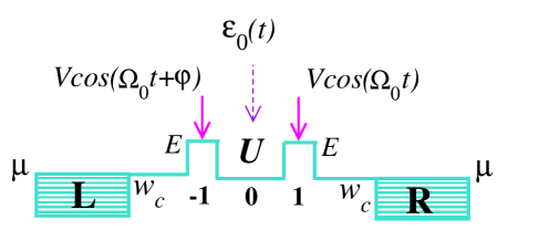
Figure 1: (Color online) Sketch of the setup. The two external ac potentials, and the induced potential at the interacting site are indicated with solid and dashed arrows, respectively.

We describe the quantum pump in terms of a generalized Anderson impurity model (see sketch of Fig. 1):

$$H(t) =\sum_{\alpha=L,R,k_{\alpha},\sigma}\varepsilon_{k_{\alpha}}n_{k_{\alpha},\sigma}-w_{c}\sum_{\alpha,k_{\alpha},\sigma}(c^{\dagger}_{k_{\alpha},\sigma}c_{l_{\alpha},\sigma}+H.c.)$$ (1)

$$-w\sum_{l=-1,\sigma}^{0}(c^{\dagger}_{l,\sigma}c_{l+1,\sigma}+H.c)$$

$$+\sum_{l=-1,\sigma}^{1}\varepsilon_{l}(t)c^{\dagger}_{l,\sigma}c_{l,\sigma}+Un_{0,\uparrow}n_{0,\downarrow},$$

being $\varepsilon_{l}(t)=\delta_{l,-1}[E+V\cos(\Omega_{0}t+\varphi)]+\delta_{l,1}[E+V\cos(\Omega_{0}t)]$. The dot with Coulomb interaction $U$ is inserted between two barriers of height $E$ at which two ac fields are applied with amplitude $V$. The degrees of freedom of the reservoirs are denoted with $k_{\alpha}$, being $\alpha=L,R$, which are at equal chemical potential $\mu$ and temperature $T=1/\beta$. The reservoirs are attached at the positions $l_{\alpha}=\pm 1$ of the central structure through hopping terms with amplitude $w_{c}$.

II.2 Charge currents

Following the procedure of Refs. lilipum , the dc-current along the structure can be expressed as a sum of an elastic and an inelastic component as follows:

$$J^{dc}=J^{el}+J^{in}=\sum_{k=-\infty}^{+\infty}\int_{-\infty}^{\infty}\frac{d\omega}{2\pi}[I^{el}(k,\omega)+I^{in}(k,\omega)],$$ (2)

where, adopting units with $e=\hbar=1$, and, to simplify, omitting explicit reference to the spin index:

$$I^{el}(k,\omega) = 2\Big{[}f(\omega-k\Omega_{0})-f(\omega)\Big{]}\Gamma(\omega)\Gamma(\omega-k\Omega_{0})$$ (3)

$$\times\sum_{l_{\alpha},l_{\alpha}^{\prime}=\pm 1}l_{\alpha}|{\cal G}_{l_{\alpha},l_{\alpha}^{\prime}}(k,\omega-k\Omega_{0})|^{2},$$

where $\Gamma(\omega)=2\pi|w_{c}|^{2}\sum_{k_{\alpha}}\delta(\omega-\varepsilon_{k_{\alpha}})$ is the tunneling rate from the structure to the reservoirs and ${\cal G}_{l,l^{\prime}}(k,\omega)$ is the $k$-th Fourier coefficient of the retarded Green’s function:

$$G^{R}_{l,l^{\prime}}(t,t^{\prime})=\sum_{k=-\infty}^{+\infty}e^{-ik\Omega_{0}t}\int_{-\infty}^{+\infty}\frac{d\omega}{2\pi}e^{-i\omega(t-t^{\prime})}{\cal G}_{l,l^{\prime}}(k,\omega),\\$$

The elastic component takes into account processes where electrons propagate coherently along the dot structure experimenting virtual absorption or emission of quanta of frequency $\Omega_{0}$ at the pumping centers. The ensuing expression coincides with the non-interacting one, except for the fact that the retarded Green’s function corresponds in the present case to the interacting system described by the full Hamiltonian (1). Instead, the inelastic contribution accounts for processes in which electrons experiment decoherence originated in the many-body interactions. It reads:

$$I^{in}(k,\omega) = 2\sum_{k^{\prime}=-\infty}^{+\infty}\mbox{Re}\Big{\{}\Gamma(\omega)\Big{[}\lambda^{>}(\omega)\Sigma^{<}_{0}(k^{\prime},\omega-k\Omega_{0})$$ (4)

$$-\lambda^{<}(\omega)\Sigma^{>}_{0}(k^{\prime},\omega-k\Omega_{0})\Big{]}\times$$

$$\Big{[}\sum_{l_{\alpha}=\pm 1}l_{\alpha}{\cal G}_{l_{\alpha},0}(k-k^{\prime},\omega-(k-k^{\prime})\Omega_{0})$$

$$\times{\cal G}^{*}_{l_{\alpha},0}(k,\omega-k\Omega_{0})\Big{]}\Big{\}},$$

being $\lambda^{<}(\omega)=if(\omega)$ and $\lambda^{>}(\omega)=-i(1-f(\omega))$, which depend on the Fermi function $f(\omega)=1/(e^{\beta(\omega-\mu)}+1)$. We have also introduced the Fourier representation of Ref. lilipum in the lesser and bigger self-energies $\Sigma^{<,>}_{0}(k,\omega)$, which describe the many-body effects due to the Coulomb interaction:

$$\Sigma^{<,>}_{0}(t,t^{\prime})=\sum_{k=-\infty}^{+\infty}e^{-ik\Omega_{0}t}\int_{-\infty}^{+\infty}\frac{d\omega}{2\pi}e^{-i\omega(t-t^{\prime})}\Sigma^{<,>}_{0}(k,\omega).$$

III Treatment of the Coulomb interaction

III.1 Time-dependent Hartree-Fock approximation

While the above expressions are in principle exact, the many-body self-energies must be calculated at some level of approximation. The lowest order in the interaction $U$ corresponds to the time-dependent-Hartree-Fock (TDHF) approximation. The many-body problem is reduced to consider Hamiltonian (1) with $U=0$ and a renormalized level given by

$$\varepsilon^{TDHF}_{l}(t)=\varepsilon_{l}(t)+\delta_{l,0}U\sum_{k=-\infty}^{+\infty}n^{TDHF}_{0,\sigma}(k)e^{-ik\Omega_{0}t}.$$ (5)

The Fourier components of the local particle density $n^{TDHF}_{0,\sigma}(k)$ must be evaluated self-consistently. This level of perturbation theory leads to a vanishing inelastic contribution $I^{in}(k,\omega)$ and it is not suitable for the description of Kondo physics. It is, however, interesting to notice that this simple approximation already introduces a non-trivial ingredient in the pumping problem. Namely, the effective emergence of an additional pumping center in the interacting site (see Fig. 1).

III.2 Second order self-energy approximation

In order to go beyond the TDHF description we consider the second order self-energy (SOSE) given by the bubble diagram of Ref. aa and generalize the procedure of that work to situations with an harmonic dependence on time. Concretely, we consider the following lesser and bigger components of the self-energy:

$$\Sigma_{0}^{>,<}(k,t-t^{\prime})=\pm iU^{2}\sum_{k_{1},k_{2}=-\infty}^{+\infty}G_{0}^{0,>,<}(k_{1},t-t^{\prime})$$

$$\times[G_{0}^{0,>,<}(k_{2},t-t^{\prime})]^{*}G_{0}^{0,>,<}(k-k_{1}+k_{2},t-t^{\prime}),$$ (6)

where the propagators are $G_{0}^{0,>,<}(k,\omega)\equiv G_{0,0}^{0,>,<}(k,\omega)$ with

$$G_{l,l^{\prime}}^{0,>,<}(k,\omega)=\sum_{\alpha,k^{\prime}}{\cal G}^{0}_{l,l_{\alpha}}(k+k^{\prime},\omega-k^{\prime}\Omega_{0})$$

$$\times\lambda^{>,<}(\omega-k^{\prime}\Omega_{0})[{\cal G}^{0}_{l^{\prime},l_{\alpha}}(k^{\prime},\omega-k^{\prime}\Omega_{0})]^{*},$$ (7)

$$G_{l,l^{\prime}}^{0,>,<}(k,t-t^{\prime})=\int_{-\infty}^{+\infty}\frac{d\omega}{2\pi}e^{-i\omega(t-t^{\prime})}G_{l,l^{\prime}}^{0,>,<}(k,\omega),$$

being the non-equilibrium retarded Green’s functions ${\cal G}^{0}_{l,l^{\prime}}(k,\omega)$, the solution of the Dyson’s equation corresponding to the Hamiltonian (1) with $U=0$ and

$$\varepsilon^{SOSE}_{l}(t)=\varepsilon_{l}(t)+\delta_{l,0}\sum_{k=-\infty}^{+\infty}\varepsilon_{0}^{eff}(k)e^{-ik\Omega_{0}t}.$$ (8)

The Fourier components of the effective potential $\varepsilon_{0}^{eff}(k)$, are determined self-consistently from the condition that the occupation of the interacting site evaluated within the SOSE approximation equals the one evaluated with (III.2), i.e.

$$n^{SOSE}_{0\sigma}(k) \equiv -i\int_{-\infty}^{+\infty}\frac{d\omega}{2\pi}G_{0}^{<}(k,\omega)$$ (9)

$$= -i\int_{-\infty}^{+\infty}\frac{d\omega}{2\pi}G_{0}^{0,<}(k,\omega),$$

where the lesser Green’s of the first equality contains the full dressing by the self-energy:

$$G_{l,l^{\prime}}^{>,<}(k,\omega) =\sum_{\alpha,k^{\prime}}{\cal G}_{l,l_{\alpha}}(k+k^{\prime},\omega-k^{\prime}\Omega_{0})\times$$

$$\lambda^{>,<}(\omega-k^{\prime}\Omega_{0})[{\cal G}_{l^{\prime},l_{\alpha}}(k^{\prime},\omega-k^{\prime}\Omega_{0})]^{*}+$$

$$\sum_{k^{\prime},k^{\prime\prime}}{\cal G}_{l,0}(k+k^{\prime}-k^{\prime\prime},\omega-(k^{\prime}-k^{\prime\prime})\Omega_{0})\times$$

$$\Sigma^{>,<}(k^{\prime\prime},\omega-k^{\prime}\Omega_{0})[{\cal G}_{l^{\prime},0}(k^{\prime},\omega-k^{\prime}\Omega_{0})]^{*},$$

while that of the second one corresponds to (III.2). The above procedure ensures the fulfillment of Friedel-Langreth sum rule in the equilibrium limit aa . Unfortunately, however, this procedure is not enough to ensure the conservation of the inelastic component of the current.

The retarded self-energy is then obtained from

$$\Sigma^{R}_{0}(k,t-t^{\prime})=\Theta(t-t^{\prime})[\Sigma_{0}^{<}(k,t-t^{\prime})-\Sigma_{0}^{>}(k,t-t^{\prime})],$$ (11)

and it is introduced in the Dyson’s equation: for the full dressed retarded Green’s functions ${\cal G}_{l,l^{\prime}}(k,\omega)$. The latter are evaluated by using the renormalization procedure of Ref. lilipum . The algorithm is combined with the use of fast Fourier transform between the variables $t-t^{\prime}\leftrightarrow\omega$.

III.3 Low amplitude and low frequencies expansion

For small pumping amplitudes and frequencies, it is possible to derive an approximate expression for the dc current that is accurate up to ${\cal O}(V^{2})$ and up to ${\cal O}(\Omega_{0})$. Such a procedure would correspond to a generalized “adiabatic approximation” within the present formalism and will allow us to get analytical expressions to gain insight on the behavior of the dc-current.

As a first step, we truncate the harmonics of the induced potentials up to $\varepsilon_{0}^{eff}(0)$ and $\varepsilon_{0}^{eff}(1)=[\varepsilon_{0}^{eff}(-1)]^{*}=V_{eff}$, and the harmonics of the self-energy up to $\Sigma(0,\omega)$ (higher harmonics involve terms ${\cal O}(V^{2})$ and ${\cal O}(U^{2}V)$). The Dyson’s equation for the retarded Green’s function reads:

$$G^{R}_{l,l^{\prime}}(t,\omega) \sim G^{0}_{l,l^{\prime}}(\omega)+$$

$$\sum_{j=-1}^{1}G^{R}_{l,j}(t,\omega+\Omega_{0})\varepsilon^{eff}_{j}(1)e^{-i\Omega_{0}t}G^{0}_{j,l^{\prime}}(\omega)+$$

$$\sum_{j=-1}^{1}G^{R}_{l,j}(t,\omega-\Omega_{0})\varepsilon^{eff}_{j}(-1)e^{i\Omega_{0}t}G^{0}_{j,l^{\prime}}(\omega),$$

where the pumping potentials contain the external time-dependent fields as well as the time-dependent potential induced by the interactions:

$$\varepsilon^{eff}_{j}(1)=V[\delta_{j,-1}e^{-i\varphi}+\delta_{j,1}]+V_{eff}\delta_{j,0},$$ (13)

with $[\varepsilon^{eff}_{j}(1)]^{*}=\varepsilon^{eff}_{j}(-1)$. The Green’s functions $G^{0}_{l,l^{\prime}}(\omega)$ correspond to the stationary part of the Hamiltonian. The solution of (III.3) up to the first order in $\varepsilon^{eff}_{j}(k)$ casts

$$G^{R}_{l,l^{\prime}}(t,\omega)=\sum_{k=-1}^{1}{\cal G}_{l,l^{\prime}}(0,\omega)e^{-i\omega_{0}t},$$ (14)

with

$${\cal G}_{l,l^{\prime}}(0,\omega) =G^{0}_{l,l^{\prime}}(\omega)$$

$${\cal G}_{l,l^{\prime}}(\pm 1,\omega) =\sum_{j=-1}^{1}G^{0}_{l,j}(\omega\pm\Omega_{0})\varepsilon^{eff}_{j}(\pm 1)G^{0}_{j,l^{\prime}}(\omega).$$ (15)

Eq. (9) leads, within this approximation, to the following self-consistency condition to evaluate $V_{eff}$:

$$V_{eff} = U\sum_{\alpha=L,R,j=-1}^{1}\int_{-\infty}^{\infty}\frac{d\omega}{2\pi}\Gamma_{0}(\omega)f(\omega)\varepsilon^{eff}_{j}(1)$$ (16)

$$\times[G^{0}_{0,j}(\omega+\Omega_{0})G^{0}_{j,l_{\alpha}}(\omega)G^{0}_{0,l_{\alpha}}(\omega)^{*}$$

$$+G^{0}_{0,l_{\alpha}}(\omega)G^{0}_{0,j}(\omega)^{*}G^{0}_{j,l_{\alpha}}(\omega-\Omega_{0})^{*}].$$

A rough estimate of the pumping potential without self-consistency is:

$$\varepsilon_{0}^{(0)}(1)\sim UV\lambda_{0}(1+e^{-i\varphi}),$$ (17)

being

$$\lambda_{0} = \int_{-\infty}^{\infty}\frac{d\omega}{2\pi}\sum_{\alpha=L,R}\int_{-\infty}^{\infty}\frac{d\omega}{2\pi}\Gamma_{0}(\omega)f(\omega)$$ (18)

$$\times[G^{0}_{0,1}(\omega+\Omega_{0})G^{0}_{1,j_{\alpha}}(\omega)G^{0}_{0,j_{\alpha}}(\omega)^{*}$$

$$+G^{0}_{0,j_{\alpha}}(\omega)G^{0}_{0,1}(\omega)^{*}G^{0}_{1,j_{\alpha}}(\omega-\Omega_{0})^{*}].$$

Thus, within this rough approximation, $V_{eff}\sim\varepsilon_{0}^{(0)}(1)=UV\lambda_{0}[1+\cos(\varphi)-i\sin(\varphi)]$. Within the self consistent procedure, however, $V_{eff}=V^{{}^{\prime}}_{eff}+iV^{{}^{\prime\prime}}_{eff}$, with both real and imaginary parts of the form $V^{{}^{\prime}(^{\prime\prime})}_{eff}\sim A^{{}^{\prime}(^{\prime\prime})}_{0}\sin(\varphi)+A^{{}^{\prime}(^{\prime\prime})}_{1}(1+\cos(\varphi))$. On the other hand, expanding the above expressions up to the first order in $\Omega_{0}$ we find $V_{eff}\sim V_{eff}^{0}+V_{eff}^{1}\Omega_{0}$.

Expanding (3) in powers of $\Omega_{0}$, casts for the first order contribution:

$$J^{dc} \sim J^{el}\sim\Omega_{0}\Gamma^{2}(\mu)$$ (19)

$$\sum_{k=-1}^{1}k\{|{\cal G}_{1,1}(k,\mu)|^{2}-|{\cal G}_{-1,-1}(k,\mu)|^{2}$$

$$+|{\cal G}_{1,-1}(k,\mu)|^{2}-|{\cal G}_{-1,1}(k,\mu)|^{2}\}.$$

Substituting the 0th order term in $\Omega_{0}$ of (15) into (19), it is found

$$J^{el} \sim\Omega_{0}\Gamma^{2}(\mu)\sum_{j\neq l}[\varepsilon^{eff}_{j}(1)\varepsilon^{eff}_{l}(1)^{*}-$$ (20)

$$\varepsilon^{eff}_{j}(-1)\varepsilon^{eff}_{l}(-1)^{*}](\lambda_{lj}-\lambda_{jl}),$$

being

$$\lambda_{jl} = \sum_{l_{\alpha}=\pm 1}l_{\alpha}G^{0}_{l_{\alpha},j}(\mu)G^{0}_{l_{\alpha},l}(\mu)^{*}\gamma_{lj}(l_{\alpha}),$$

$$\gamma_{lj}(-1) = \sum_{l_{\alpha}=\pm 1}G^{0}_{j,l_{\alpha}}(\mu)G^{0}_{l,l_{\alpha}}(\mu)^{*},$$

$$\gamma_{lj}(1) = \sum_{l_{\alpha}=\pm 1}G^{0}_{j,l_{\alpha}}(\mu)G^{0}_{l,-l_{\alpha}}(\mu)^{*}$$ (21)

In the case of the rough estimate for the induced pumping potential $\varepsilon_{0}^{(0)}(1)$ defined above, a relation between the current and the phase-lag of the form $J^{el}\propto\sin(\varphi)$, as in the non-interacting case, is obtained. However, when the pumping potential is evaluated self-consistently, the current behaves as follows:

$$J^{dc} \sim J^{el}\sim\Omega_{0}\frac{(\Gamma^{el})^{2}}{(\Gamma_{0})^{4}}V\Big{[}V\sin(\varphi)\lambda^{el}_{1}$$ (22)

$$+\Big{(}V^{{}^{\prime}}_{0}\sin(\varphi)(\cos(\varphi)+1)+V^{{}^{\prime\prime}}_{0}\sin^{2}(\varphi)\Big{)}\lambda^{el}_{2}\Big{]},$$

where we have defined $\Gamma^{el}=\Gamma(\mu)$, being $\Gamma_{0}=4|w|^{2}/\Gamma(\mu)$, which is approximately the effective tunneling rate from the interacting site to the leads. The dimensionless functions $\lambda_{i}^{el}$ as well as $V^{{}^{\prime}}_{0},V^{{}^{\prime\prime}}_{0}$ depend on $V_{eff}$ and on the parameters $\lambda_{lj}$ of eq. (III.3). It is important to note that Eq. (22) reduces to the the non-interacting result $J^{dc}\sim V^{2}\sin(\varphi)$ originally proposed in Ref. brouwer , for $V_{0}^{{}^{\prime}}=V_{0}^{{}^{\prime\prime}}=0$. Such a dependence on $\varphi$ has been observed experimentally in Ref. switkes and is a manifestation of quantum interference between processes of coherent emission and absorption of quanta at the two pumping centers. In the interacting system the terms $\propto\lambda_{2}^{el}$ of Eq.(22) are a consequence of additional interference with scattering events at the pumping center induced by the interactions.

The inelastic contribution exhibits the same structure, except for a different prefactor $\Gamma^{in}=-2\mbox{Im}[\Sigma^{eq}_{0}(\mu)]$, being $\Sigma^{eq}_{0}(\omega)\sim\Sigma^{R}_{0}(0,\omega)$ the SOSE of the system with $V=0$, instead of $\Gamma^{el}$. For low $T$, $\Gamma^{in}\sim(\omega-\mu)^{2}$, thus, for low $\Omega_{0}$ $J^{in}\sim 0$ and the elastic processes account for the full dc transport.

IV Results

IV.1 Weakly interacting regime

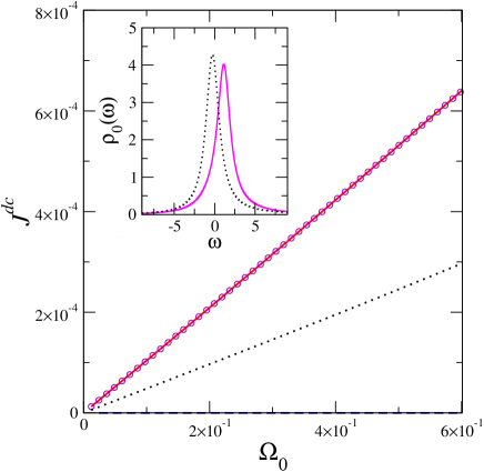
Figure 2: (Color online) $J^{el}$ (solid line) , $J^{in}$ (dashed line) and $J^{dc}$ (circles) for $\varphi=\pi/2$, as functions of the driving frequency $\Omega_{0}$ for $U=1$. The inelastic component is $J^{in}\sim 0$. The dc-current for the non-interacting system ($U=0$) is also shown in dotted lines for comparison. The corresponding local densities of states at the interacting site $\rho_{0}(\omega)$ are indicated in the inset (solid lines), along with the non-interacting one (dotted lines).Other parameters are $E=2,w=2,w_{c}=8$, $V=0.4$ and $\mu=2$. (Energies, frequencies and currents are expressed in units of $\Gamma_{0}$).

We begin with the analysis of the effect of the interactions in the behavior of $J_{dc}$ as a function of $\Omega_{0}$ at $T=0$ for a given chemical potential $\mu$ and phase-lag $\varphi$. In Fig. 2 we present the behavior of the different contributions to $J^{dc}$ obtained from the numerical solution of the full Dyson’s equation retaining self-energy components $\Sigma_{0}^{>,<}(k,\omega)$ up to $|k|=2$, with the self-consistent evaluation of $\varepsilon_{0}^{eff}(0)$, and $\varepsilon_{0}^{eff}(1)\equiv V_{eff}$. Energies, frequencies and currents are expressed in units of $\Gamma_{0}$. The inset shows the corresponding local density of states at the interacting site $\rho_{0}(\omega)=-2\mbox{Im}[{\cal G}_{0,0}(0,\omega)]$ along with the density of states corresponding to the non-interacting system ($U=0$). The position of the resonant peak experiments a shift equal to $\varepsilon_{eff}(0)$. For low $U$ the effects of $\Sigma(k,\omega)$ are vanishingly small and the description effectively reduces to TDHF. The induced $V_{eff}$ is also very small ($V_{eff}\sim 1\times 10^{-3}<<V$). For low $U$, the inelastic contribution to the current (${\cal O}(U^{2})$) is negligible. Therefore, within this regime, $J^{dc}$ is qualitatively similar to the non-interacting one, shown in dotted line. As the hybridization between the dot and the side reservoirs is sizable, the resonant peak is wide and the “adiabatic” ($\propto\Omega_{0}$ behavior) is observed within a wide range of $\Omega_{0}$.

IV.2 Kondo regime

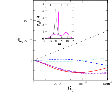
Figure 3: (Color online) $J^{el}$ (solid line) , $J^{in}$ (dashed line) and $J^{dc}$ (circles) for $\varphi=\pi/2$, as functions of the driving frequency $\Omega_{0}$ for $U=10$. The details are the same as in Fig. 2.

Let us now analyze the more subtle Kondo regime, which takes place at higher $U$. In Fig 3 we show a series of plots similar to those of Fig. 2 but corresponding to a value of $U$ for which the Kondo effect takes place. For these parameters, the density of states at the interacting site $\rho_{0}(\omega)$ exhibits the characteristic Kondo resonance at $\omega=0$ with the two high-energy side features centered at $\omega=\pm U/2$ (see inset). As a function of $\Omega_{0}$ the behavior of $J^{dc}$ significantly departs from the non-interacting one in this regime and there are several issues to comment in connection to Fig. 3. First, it is clear that self-energy effects now play an important role. This is evident in the drastic changes experimented by the density of states as well as in the fact that the current departs from the behavior predicted by the TDHF approximation, which is shown in light dot-dashed line in the figure.

The second feature to remark is that, although inelastic processes are negligible for low $\Omega_{0}$, as discussed in Section III.C, they become sizable as $\Omega_{0}$ increases even at $T=0$ (see dashed line of the main frame of Fig. 3).

The third remarkable issue is the lose of the “adiabatic” behavior, namely, the departure from the linear dependence in $\Omega_{0}$. We identify two ingredients that contribute to this effect: (i) The first one is the induced pumping potential at the interacting site, which becomes sizable $V_{eff}>1\times 10^{-2}$ and changes significantly with $\Omega_{0}$. This feature manifests itself even at the TDHF level, in which case the range of pumping frequencies where $J^{dc(TDHF)}\propto\Omega_{0}$ becomes very narrow ($\Omega_{0}<2\times 10^{-2}$). (ii) The other ingredient is the development of the Kondo resonance. Recalling that the underlying assumption for low frequency expansions like the one leading to Eq. (22) is that the typical width of the energy levels of the structure is $\tau^{-1}>>\Omega_{0}$, it can be understood that the reduction of the width of the resonant level due to the Kondo effect originates a concomitant reduction of the range of $\Omega_{0}$ for the “adiabatic” behavior to be observed. For the parameters of Fig. 3, which correspond to $T_{K}\sim 0.5$, such a linear behavior is not captured even close to the lowest pumping frequency considered ($\Omega_{0}=1\times 10^{-2}$).

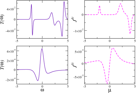
Figure 4: (Color online) “Transmission function” $T(\omega)$ for a noninteracting structure with $\Omega_{0}=0.1$ and $w_{c}=0.64$ (upper left panel) and $w_{c}=8$ (lower left panel). Other details are the same as in Fig. 2.

The final issue worth of mention is the inversion in the sign of the current with respect to the non-interacting case. In general, even in the simpler case of a system without many-body interactions, the issue of the sign of the current is one of the most delicate features to predict in a problem of quantum pumping. In the case of structures with low hybridization with the contacts presenting a landscape of well separated resonances, the issue of the sign of the current has been analyzed in detail in Refs. mobu, ; lilipum, ; lilidir, . In those works, the origin for the sign inversion of the current has been identified to be the interference between two resonant electronic levels mixed by a high pumping frequency. In order to gain insight on the different processes involved in the present problem, let us first analyze the behavior of the sign of the current in the non-interacting limit of our setup of Fig. 1. In that case the dc current (2) can be also written as follows lilipum :

$$J^{dc}_{non-int}=\int_{-\infty}^{+\infty}d\omega f(\omega)T(\omega),$$ (23)

where the “transmission” function $T(\omega)$ depends on the Green’s functions of the system with $U=0$. Plots of the function $T(\omega)$ and its integral between $-\infty$ and $\mu$, which is equivalent to $J^{dc}_{non-int}$ at zero temperature for two different hybridizations $w_{c}$, are shown in Fig. 4. In the upper panels, corresponding to a small $w_{c}$ three features associated to the three eigenvalues of the tight-binding structure with three sites $l=-1,0,1$, can be distinguished. Instead, for the higher $w_{c}$ chosen to capture the Kondo regime used in Figs. 2 and 3, the three levels of the uncoupled structure are mixed and only one feature can be distinguished. As a consequence of the ensuing combination of quantum states, the transmission function as well as the current changes the sign within a wide range of $\mu$ with respect to the weakly coupled structure.

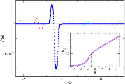
Figure 5: (Color online) Integrand $I(\omega)$ for $\Omega_{0}=0.1$ and $U=10$. Different plots correspond to different equidistant values of the chemical potential $-2\leq\mu\leq 0.4$. In the inset, the mean occupation per spin of the dot is shown as a function of the chemical potential. Other parameters are as in Fig. 2.

In the case of the interacting system, we analyze the behavior of the function $I(\omega)=\sum_{k}[I^{el}(k,\omega)+I^{in}(k,\omega)]$, which, when integrated over $\omega$ gives the total dc current. The behavior of this function within the Kondo regime is shown in Fig. 5. Unlike the function $T(\omega)$ defined for the non-interaction system, the function $I(\omega)$ changes as the chemical potential changes. For this reason, several plots corresponding to different values of the chemical potential, for which we have verified that the Kondo resonance is developed, are shown in the figure. For each $\mu$ there is a feature in $I(\omega)$ around $\omega\sim\mu$ which precisely indicates the electronic transmission through the Kondo resonance. Notice that these features are very narrow and resemble the lowest energy one of the upper left panel of Fig. 4, which corresponds to a resonance for a dot with low hybridization with the reservoirs. Interestingly, for $\mu\sim-1$, $I(\omega)$ experiments a phase shift of $\pi$, leading to a concomitant change of sign in the dc current. This particular value of the chemical potential corresponds to a charge population per spin of the dot $n_{0}\equiv n^{SOSE}_{0,\sigma}(0)\sim 1/2$.

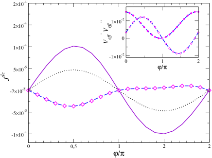
Figure 6: (Color online) $J^{dc}$ for $\Omega_{0}=0.1$ as a function of the phase-lag $\varphi$ for $U=1$ (thick solid line), and $U=10$ (thick dashed line). The current corresponding to the non-interacting dot (with $U=0$) is shown in dotted line, for comparison. The symbols are fits with a function $A_{0}\sin(\varphi)+A_{1}\sin^{2}(\varphi)+A_{2}\sin(\varphi)(1+\cos(\varphi))$, suggested by eq. (22). Inset: Effective potential $V_{eff}=V_{eff}^{\prime}+iV_{eff}^{\prime\prime}$ along with fits in symbols with the function: $A_{0}\sin(\varphi)+A_{1}(1+\cos(\varphi))$. Other details are as in Fig. 2.

We show in Fig. 6 the behavior of the dc-current as a function of the phase-lag. The limiting case of $U=0$ is plotted in dotted lines in Fig. 6. For low Coulomb interaction (see plot in solid thick line) the induced effective pumping potential is small and the behavior of the dc-current is qualitatively the same as the one corresponding to the non-interacting case. For increasing $U$, the induced pumping amplitude $V_{eff}$ becomes sizable. Within the self-consistent procedure, this is a complex function of $\varphi$ with real and imaginary parts $V^{{}^{\prime}}_{eff}$ and $V^{{}^{\prime\prime}}_{eff}$ displaying the functional structure of $\varphi$ suggested by the perturbative solution leading to Eq. (22). The ensuing curve $J^{dc}\;\mbox{vs}\;\varphi$ also shows the pattern predicted by Eq. (22). Notice that the dc-current, as well as $V_{eff}$ can be fitted with an excellent degree of accuracy by functions of $\varphi$ with the structure suggested by this equation (see symbols in Fig. 6). An striking feature observed in this figure as well as in the analytical expression (22) is the breaking of the symmetry $\varphi\rightarrow-\varphi$ in the behavior of the dc-current. On general physical grounds, the symmetry of the problem in the case of identical pumping amplitudes at the two barriers indicates that $J^{dc}(\varphi)\rightarrow-J^{dc}(-\varphi)$. However, the many-body treatment adopted in the present work breaks such symmetry for high enough induced $V_{eff}$, even at the level of the simple self-consistent TDHF approximation, i.e. even disregarding self-energy effects. The self-consistent evaluation of higher harmonics (we recall that we truncate at $|k|=2$), and additional self-energy and vertex corrections that we have not taken into account are expected to restore such symmetry. In any case, our results should be interpreted as a piece of evidence on the departure from the $J^{dc}\propto\sin(\varphi)$ behavior induced by the interactions.

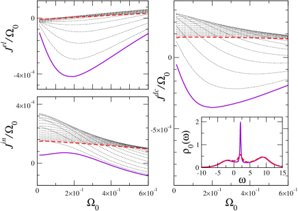
Figure 7: (Color online) $J^{el}/\Omega_{0}$ (top left), $J^{in}/\Omega_{0}$ (bottom left) and $J^{dc}/\Omega_{0}$ (right) as functions of the pumping frequency $\Omega_{0}$ for $20$ values of equally spaced temperatures in the range $0.04\leq T/T_{K}\leq 0.8$ and Coulomb interaction $U=10$. The lowest and highest temperatures are indicated in thick solid and dashed lines, respectively. The local density of states of the dot, $\rho_{0}(\omega)$, is depicted in the inset for the lowest and highest temperatures. Other details are as in Fig. 2

So far, we have focused in the case of temperature $T=0$, where inelastic effects play an insignificant role at low $\Omega_{0}$. To finalize, we analyze in what follows inelastic effects, which become relevant at all frequencies at finite $T$. The evolution of the dc-current as a function of $\Omega_{0}$ as the temperature grows within a range $0<T<T_{K}$ is analyzed in Fig. 7. At first glance, it becomes apparent how the dominant contribution at low $\Omega_{0}$ is $J^{el}$ at the lowest $T$, while it turns to be $J^{in}$ for the highest ones. The elastic contribution vanishes as the Kondo resonance disappears while the inelastic one increases due to the corresponding grow of $\Gamma^{in}$. The latter increment translates into the inverse time $\tau^{-1}$, thus increasing the range of $\Omega_{0}$ where the behavior $J^{dc}\propto\Omega_{0}$ holds. In fact, notice that the range of low $\Omega_{0}$ where the plots of Fig. 4 look horizontal increases with increasing $T$.

V Summary and conclusions

To conclude, we have analyzed a simple model for an interacting quantum pump by means of non-equilibrium Green’s function techniques and within a second order self-energy approximation. We have shown that the effective time-dependent scattering center induced by the interactions generates interference effects, which should be detected in a $J^{dc}\;\mbox{vs}\;\varphi$ experimental curve, following the pattern predicted by Eq. (22). We have shown that the Kondo effect manifests itself in the $J^{dc}\;\mbox{vs}\;\Omega_{0}$ behavior, which could be also detected in future experiments. Below the Kondo temperature, $T_{K}$, the Kondo resonance enables the elastic transport of electrons, however the frequency range within which $J^{dc}$ behaves linear in $\Omega_{0}$ is extremely narrow. As the temperature grows, inelastic scattering becomes dominant and this range becomes wider.

VI Acknowledgments

We thank C. Urbina and J. Splettstoesser for constructive comments. We acknowledge support from CONICET, Argentina, FIS2006-08533-C03-02, the “RyC” program from MCEyC, grant DGA for Groups of Excelence of Spain and the hospitality of Boston University (LA), as well as FIS2005-06255 from MCEyC Spain (ALY and AMR).

References

- (1) M. Switkes, C. M. Marcus, K. Campman, A. C. Gossard, Science 283, 1905 (1999).
- (2) L. J. Geerligs, V. F. Anderegg, P. A. M. Holweg, J. E. Mooij, H. Pothier, D. Esteve, C. Urbina and M. H. Devoret, Phys. Rev. Lett. 64, 2691 (1990); L. DiCarlo, C. M. Marcus and J. S. Harris, Phys. Rev. Lett. 91, 246804 (2003).
- (3) M. D. Blumenthal, B. Kaestner, L. Li, S. Giblin, T. J. B. M. Hanssen, M. Pepper, D. Anderson, G. Jones and D. A. Ritchie, Nature Physics 3, 343 (2007).
- (4) D. Goldhaber-Gordon et al, Nature (London) 391, 156 (1998).
- (5) B. Babic, T. Kontos and C. Schonenberger, Physical Review B 70, 235419, (2004); P. Jarillo-Herrero, et al, Nature 434, 484(2005).
- (6) P.M. Billangeon, F. Pierre, H. Bouchiat, and R. Deblock, Phys. Rev. Lett. 98, 126802 (2007); S. Russo, J. Tobiska, T. M. Klapwijk, and A. F. Morpurgo, Phys. Rev. Lett. 99, 086601 (2007).
- (7) M. Büttiker, H. Thomas, A. Prêtre, Z. Phys. B 94, 133 (1994).
- (8) P. W. Brouwer, Phys. Rev. B 58, R10135 (1998).
- (9) P.W. Brouwer, Phys. Rev. B 63, 121303 (2001); M.L. Polianski and P.W. Brouwer, Phys. Rev. B 64, 075304 (2001).
- (10) M. Moskalets and M. Büttiker, Phys. Rev. B 66, 205320 (2002); Phys. Rev. B 69, 205316 (2004).
- (11) I. L. Aleiner and A. V. Andreev, Phys. Rev. Lett. 81, 1286 (1998); F. Zhou, B. Spivak, and B. Altshuler, Phys. Rev. Lett. 82, 608 (1999); J. E. Avron, A. Elgart, G. M. Graf, and L. Sadun, Phys. Rev. B 62, R10618 (2000); Phys. Rev. Lett. 87, 236601 (2001); J. Math. Phys. 43, 3415 (2002). O. Entin-Wohlman, A. Aharony, and Y. Levinson, Phys. Rev. B 65, 195411 (2002); V. Kashcheyevs, A. Aharony, and O. Entin-Wohlman, Phys. Rev. B 69, 195301 (2004).
- (12) B. Wang and J. Wang, Phys. Rev. B 65, 233315 (2002); M. N. Kiselev, K. Kikoin, R. I. Shekhter, and V. M. Vinokur, Phys. Rev. B 74, 233403 (2006); E. Sela and Y. Oreg, Phys. Rev. Lett. 96, 166802 (2006).
- (13) T. Aono, Phys. Rev. Lett. 93, 116601 (2004); J. Splettstoesser, M. Governale, J. König and R. Fazio, Phys. Rev. Lett. 95, 246803 (2005).
- (14) K. Das, cond-mat/0710.2953.
- (15) A. Levy Yeyati, A. Martín-Rodero, and F. Flores, Phys. Rev. Lett. 71, 2991 (1993).
- (16) L. Arrachea, Phys. Rev. B 72, 125349 (2005); Phys. Rev. B 75, 035319 (2007).
- (17) A. Oguri, Phys. Rev. B 52, 16727 (1995); R. López, R. Aguado, G. Platero, and C. Tejedor Phys. Rev. Lett. 81, 4688 (1998); A. Levy Yeyati, F. Flores, and A. Martín-Rodero Phys. Rev. Lett. 83, 600 (1999).
- (18) L. Arrachea and M. Moskalets Phys. Rev. B 74, 245322 (2006).
- (19) L. Arrachea, C. Naón, and M. Salvay, Phys. Rev. B 76, 165401 (2007).