Generating entangled coherent state of two cavity modes in three-level $\Lambda$-type atomic system

Abstract

In this paper, we present a scheme to generate an entangled coherent state by considering a three-level $"\Lambda"$ type atom interacting with a two-mode cavity driven by classical fields. The two-mode entangled coherent state can be obtained under large detuning condition. Considering the cavity decay, an analytical solution is deduced.

.1 I. Introduction

Entanglement between quantum systems is recognized nowadays as a key ingredient for testing quantum mechanics versus local hidden-variable theory Hybrid-32 . Entanglement as a valuable resource has been used in quantum information processing such as quantum computation Hybrid-1 , quantum sweeping and teleportation Hybrid-2 . As macroscopic nonclassical states, Schr$\ddot{o}$dinger cat states and entangled coherent states have always been an attractive topic. In quantum optics, these two kinds of states are described as superpositions of different coherent states and superpositions of two-mode coherent states, respectively. It has been shown that such superposition states have many practical applications in quantum information processing Hybrid-4 . So far, a variety of physical systems presenting entangled coherent states have been investigated Hybrid-7 ; Hybrid-24 ; Hybrid-9 ; Hybrid-10 ; Hybrid-25 ; Hybrid-29 ; Hybrid-12 . Sanders Hybrid-7 presented a method for generating an entangled coherent state with equal weighting factors by using a nonlinear Kerr medium placed in one arm of the nonlinear Mach-Zehnder interferometer. Wielinga et al. Hybrid-24 modified this scheme via an optical tunnelling device instead of the Kerr medium to generate entangled coherent states with a variable weighting factor. Schemes have also been proposed for generating such entangled coherent states using trapped ions Hybrid-9 by controlling the quantized ion motion precisely.

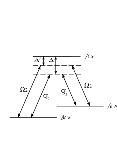
Figure 1: Schematic diagram of a three-level $\Lambda-$type atom interacting with two cavity modes and two classic fields with detunings $\Delta$ and $\Delta^{\prime}$, respectively.

On the other hand, cavity QED, with Rydberg atoms interacting with an electromagnetic field inside a cavity, has also been proved to be a promising environment to generate quantum states. In the context of cavity QED, several schemes have been proposed to generate such superposition coherent states Hybrid-10 ; Hybrid-25 ; Hybrid-29 ; Hybrid-12 . Ref. Hybrid-25 showed that entangled coherent states can be generated by the state-selective measurement on a two-level atom interacting with a two-mode field. Recently, Wang and Duan Hybrid-29 studied the generation of multipartite and multidimensional cat states by reflecting coherent pulses successively from a single-atom cavity. Solano et al. Hybrid-12 proposed a method for generating entangled coherent states by considering a two-level atom cavity QED driven by a strong classic field. However, the two cavity modes in this scheme interact with the same atomic transitions, and thus can not be easily manipulated.

In our research, we present an alternative method to prepare two modes of cavity in an entangled coherent state with the context of cavity QED. Based on the nonresonant interaction of a three-level $"\Lambda"$ type atom with two cavity modes and two classic fields, we can obtain the entangled coherent states. Compared with Ref. Hybrid-12 , the two cavity modes in our research interact with different atomic transitions so that they are easy to be recognized and manipulated. Furthermore, we work on the large detuning condition, so the decoherence induced by the spontaneous emission of excited level $|c\rangle$ can be ignored. Our scheme can also be generalized to generate multidimensional entangled coherent state with the assistance of another two-level atom in two-photon process.

.2 II. The theoretical model and calculation

The system we consider is a three-level atom in $\Lambda$ configuration placed inside a two-mode field cavity. The level structure of the atom is depicted in Fig.1, where the two atomic transitions $|c\rangle\leftrightarrow|e\rangle$ and $|c\rangle\leftrightarrow|g\rangle$ interact with the two cavity modes with the same detuning $\Delta$ but with different coupling constants $g_{1}$ and $g_{2}$, respectively. The two atomic transitions $|c\rangle\leftrightarrow|e\rangle$ and $|c\rangle\leftrightarrow|g\rangle$ are also driven by two classical fields with detuning $\Delta^{\prime}$, and $\Omega_{1}$ and $\Omega_{2}$ are the Rabi frequencies of the two classical fields. The Hamiltonian for the system can be written as

$$H = \hbar w_{e}|e\rangle\langle e|+\hbar w_{c}|c\rangle\langle c|+\hbar w_{1}a_{1}^{\dagger}a_{1}+\hbar w_{2}a_{2}^{\dagger}a_{2}$$ (1)

$$+\hbar g_{1}(a_{1}^{\dagger}|e\rangle\langle c|+a_{1}|c\rangle\langle e|)+\hbar g_{2}(a_{2}^{\dagger}|g\rangle\langle c|+a_{2}|c\rangle\langle g|)$$

$$+\hbar\Omega_{1}(e^{-i(w_{c}-w_{e}-\Delta^{\prime})t}|c\rangle\langle e|+H.c.)+\hbar\Omega_{2}(e^{-i(w_{c}-\Delta^{\prime})t}|c\rangle\langle g|+H.c.),$$

where $a_{i}^{\dagger}$ and $a_{i}$ are the creation and annihilation operators for the cavity fields of frequencies $w_{i}$ (i=1,2), while $w_{c}$ and $w_{e}$ are the Bohr frequencies associated with the two atomic transitions $|c\rangle\leftrightarrow|g\rangle$ and $|e\rangle\leftrightarrow|g\rangle$, respectively.

We consider the large detuning domain

$$\left(\frac{\Omega_{1}}{\Delta^{\prime}},\frac{\Omega_{2}}{\Delta^{\prime}},\frac{g_{1}}{\Delta},\frac{g_{2}}{\Delta}\right)\ll 1.$$ (2)

After adiabatically eliminating the excited level $|c\rangle$, we derive the effective Hamiltonian as follows Hybrid-14

$$H_{eff}{=}-\hbar g_{eff}(a_{1}^{\dagger}a_{2}\sigma^{\dagger}+a_{1}a_{2}^{\dagger}\sigma)-\hbar\Omega_{eff}(\sigma^{\dagger}+\sigma),$$ (3)

where $g_{eff}{=}\frac{g_{1}g_{2}}{\Delta}$, $\Omega_{eff}{=}\frac{\Omega_{1}\Omega_{2}}{\Delta^{\prime}}$; $\sigma^{\dagger}{=}\left|e\right\rangle\left\langle g\right|$ and $\sigma{=}\left|g\right\rangle\left\langle e\right|$ are raising and lowering atomic operators, respectively. In Eq.(3) we have assumed that the Stark shifts can be corrected by retuning the laser frequencies Hybrid-22 .

In the strong driving regime $\Omega_{eff}{\gg}g_{eff}$, we choose $H_{eff}^{0}{=}-\hbar\Omega_{eff}(\sigma^{\dagger}+\sigma)$ and $H_{eff}^{I}{=}-\hbar g_{eff}(a_{1}^{\dagger}a_{2}\sigma^{+}+a_{1}a_{2}^{\dagger}\sigma)$. By performing the unitary transformation $U{=}e^{-\frac{i}{\hbar}H_{eff}^{0}t}$ on $H_{eff}^{I}$, in which we neglect the terms that oscillate with high frequencies, the Hamiltonian reads

$$H_{eff}^{int}=-\frac{\hbar g_{eff}}{2}(a_{1}^{\dagger}a_{2}+a_{1}a_{2}^{\dagger})(\sigma^{\dagger}+\sigma).$$ (4)

We recognize the field Hamiltonian part $-\frac{\hbar g_{eff}}{2}(a_{1}^{\dagger}a_{2}+a_{1}a_{2}^{\dagger})$ is the generator of the SU(2) coherent state Hybrid-27 . Here, we are interested in using the Hamiltonian of Eq.(4) to entangle the two cavity modes through the interaction with the atom. For this purpose we consider the case that the atom state is initially prepared in the ground state $|g\rangle$, while both of the two cavity fields are in coherent states $|\alpha\rangle$ and $\beta\rangle$, respectively. Thus the initial state of the system is

$$|\Psi(0)\rangle=|g\rangle\otimes|\alpha,\beta\rangle.$$ (5)

On the basis of $|\pm\rangle=\frac{1}{\sqrt{2}}(|g\rangle\pm|e\rangle)$, which are the eigenstates of $\sigma+\sigma^{\dagger}$ with eigenvalues $\pm 1$, the time evolution of the system is given by

$$|\Psi(t)\rangle =e^{\frac{-i}{\hbar}H_{eff}^{int}t}|\Psi(0)\rangle$$ (6)

$$=\frac{1}{\sqrt{2}}e^{\frac{ig_{eff}t}{2}(K_{+}+K_{-})}|+,\alpha,\beta\rangle+\frac{1}{\sqrt{2}}e^{\frac{-ig_{eff}t}{2}(K_{+}+K_{-})}|-,\alpha,\beta\rangle,$$

where $K_{+}=a_{1}^{\dagger}a_{2}$, $K_{-}=a_{1}a_{2}^{\dagger}$. These operators satisfy the SU(2) commutation relations, i.e. $[K_{-},K_{+}]=-2K_{0}$, $[K_{0},K_{+}]=K_{+}$, $[K_{0},K_{-}]=-K_{-}$, with $K_{0}=\frac{1}{2}(a_{1}^{\dagger}a_{1}-a_{2}^{\dagger}a_{2})$. Thus we can use the SU(2) Lie algebra Hybrid-15 to expand the unitary evolution operator $e^{\pm\frac{ig_{eff}t}{2}(K_{+}+K_{-})}$ as

$$e^{\pm\frac{ig_{eff}t}{2}(K_{+}+K_{-})}=e^{\pm x_{+}K_{+}}e^{K_{0}\ln{x_{0}}}e^{\pm x_{-}K_{-}},$$ (7)

in which

$$x_{0} = \{\cosh{\frac{ig_{eff}t}{2}}\}^{-2},$$

$$x_{+} = x_{-}=\tanh{\frac{ig_{eff}t}{2}}.$$

Using Eq.(7) we can conveniently derive the evolution of the system as

$$|\Psi(t)\rangle=\frac{1}{\sqrt{2}}|+\rangle|\tilde{\alpha},\tilde{\beta}\rangle+\frac{1}{\sqrt{2}}|-\rangle|\tilde{\alpha}^{\ast},\tilde{\beta}^{\ast}\rangle,$$ (8)

with

$$\tilde{\alpha} = \alpha\cos{\frac{g_{eff}t}{2}}+i\beta\sin{\frac{g_{eff}t}{2}},$$

$$\tilde{\beta} = \beta\cos{\frac{g_{eff}t}{2}}+i\alpha\sin{\frac{g_{eff}t}{2}}.$$

We now change the basis back to original atomic states

$$|\Psi(t)\rangle{=}\frac{1}{2}|g\rangle(|\tilde{\alpha},\tilde{\beta}\rangle+|\tilde{\alpha}^{\ast},\tilde{\beta}^{\ast}\rangle)+\frac{1}{2}|e\rangle(|\tilde{\alpha},\tilde{\beta}\rangle-|\tilde{\alpha}^{\ast},\tilde{\beta}^{\ast}\rangle).$$ (9)

When the atom comes out from the two-mode cavity, we can use level-selective ionizing counters to detect the atomic state. If the internal state of atom is detected to be in the state $|g\rangle$ or $|e\rangle$, Eq.(9) will project the two-mode cavity into

$$|\Psi_{f}(t)\rangle{=}\frac{1}{\sqrt{M}}(|\tilde{\alpha},\tilde{\beta}\rangle\pm|\tilde{\alpha}^{\ast},\tilde{\beta}^{\ast}\rangle),$$ (10)

where $M$ is normalization factor such that

$$M=2\pm[exp(-|\tilde{\alpha}|^{2}-|\tilde{\beta}|^{2}+\tilde{\alpha}^{\ast^{2}}+\tilde{\beta}^{\ast^{2}})+exp(-|\tilde{\alpha}|^{2}-|\tilde{\beta}|^{2}+\tilde{\alpha}^{2}+\tilde{\beta}^{2})].$$ (11)

By this way we obtain a superposition of two two-mode coherent states. It is interesting to note that under certain conditions on the amplitudes of two coherent states, such superposition state can exhibit nonclassical effects such as violation of the Cauchy-Schwartz inequality and two-mode squeezing Hybrid-16 . On the other hand, the interaction time of the atom in the cavity can be controlled as $m\pi/g_{eff}$ by using a velocity selector, where $m$ is odd number. Then we can obtain two-mode even and odd coherent states as $|\Psi_{f}(t)\rangle{=}\frac{1}{\sqrt{M}}(|i\beta,i\alpha\rangle\pm|-i\beta,-i\alpha\rangle)$ Hybrid-16 . It has been proved that these even and odd coherent states exist strong correlations between two modes.

Now we try to estimate the entanglement of Eq.(10). Recently, different entanglement criteria for two-mode systems have been proposed in Hybrid-20 ; Hybrid-18 ; Hybrid-19 . Here, we choose constructing normalized and orthogonal basis and then use concurrence to evaluate the entanglement proposed in Hybrid-20 ; Hybrid-26 . According to Ref. Hybrid-26 , the concurrence of Eq.(10) is given by

$$C=\frac{2}{|M|}\sqrt{(1-|p_{1}|^{2})(1-|p_{2}|^{2})}.$$ (12)

where $P_{1}=e^{-|\tilde{\alpha}|^{2}+\tilde{\alpha}^{\ast^{2}}}$ and $P_{2}=e^{-|\tilde{\beta}|^{2}+\tilde{\beta}^{\ast^{2}}}$.

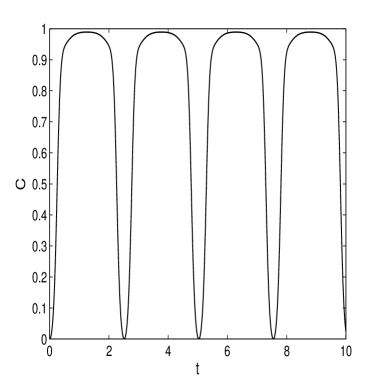
Figure 2: The time evolution of the degree of the entanglement with $g_{eff}=2.5$, $\alpha=1$, $\beta=1.5$.

Fig.2 shows the time evolution of the concurrence. Here the positive sign has been chosen for Eq.(10). We see that under this group of parameters of the two modes, concurrence oscillates periodically with time. From Eq.(10), it is easy to see that the state is entangled at any other time, except when $\tilde{\alpha}$ and $\tilde{\beta}$ are real, namely $t=n\pi/g_{eff}$ (where $n$ is even number).

.3 III. Analytical solution including cavity decay

Due to the large detuning, the excited atomic level $|c\rangle$ do not participate in the interaction. Therefore, the spontaneous emission atomic level can be ignored. Now, we discuss the time evolution of the system under the cavity losses. For simplicity, we assume the losses of the two cavity modes are equal. By including the cavity damping terms in the equation of motion for the density operators, the mast equation can be written as

$$\dot{\rho}=\frac{-i}{\hbar}[H_{eff},\rho]+L_{1}\rho+L_{2}\rho,$$ (13)

where $L_{i}=\frac{k}{2}(2a_{i}\rho a_{i}^{\dagger}-a_{i}^{\dagger}a_{i}\rho-\rho a_{i}^{\dagger}a_{i})$ for $i=1,2$.

This equation can be solved by Lie algebras Hybrid-15 and superoperator technique Hybrid-23 . When the initial state is prepared in $|g,\alpha,\beta\rangle$, we can obtain the analytical solution of the system as follows

$$\rho = \frac{1}{2}|+,\tilde{\alpha}e^{\frac{-kt}{2}},\tilde{\beta}e^{\frac{-kt}{2}}\rangle\langle+,\tilde{\alpha}e^{\frac{-kt}{2}},\tilde{\beta}e^{\frac{-kt}{2}}|+\frac{1}{2}|-,\tilde{\alpha}^{*}e^{\frac{-kt}{2}},\tilde{\beta}^{*}e^{\frac{-kt}{2}}\rangle\langle-,\tilde{\alpha}^{*}e^{\frac{-kt}{2}},\tilde{\beta}^{*}e^{\frac{-kt}{2}}|$$

$$+\frac{1}{2}\eta|+,\tilde{\alpha}e^{\frac{-kt}{2}},\tilde{\beta}e^{\frac{-kt}{2}}\rangle\langle-,\tilde{\alpha}^{*}e^{\frac{-kt}{2}},\tilde{\beta}^{*}e^{\frac{-kt}{2}}|+\frac{1}{2}\eta^{*}|-,\tilde{\alpha}^{*}e^{\frac{-kt}{2}},\tilde{\beta}^{*}e^{\frac{-kt}{2}}\rangle\langle+,\tilde{\alpha}e^{\frac{-kt}{2}},\tilde{\beta}e^{\frac{-kt}{2}}|,$$

where

$$\eta{=}exp[-4\lambda_{1}\tilde{\alpha}\tilde{\beta}+(|\tilde{\alpha}|^{2}+|\tilde{\beta}|^{2})(e^{-kt}-1)+2\lambda_{2}(\tilde{\alpha}^{2}+\tilde{\beta}^{2})],$$

$$\lambda_{1}{=}\frac{kg_{eff}\cos(g_{eff}t)-k^{2}\sin(g_{eff}t)-kg_{eff}e^{-kt}}{2i(k^{2}+g_{eff}^{2})},$$

$$\lambda_{2}{=}\frac{k^{2}\cos(g_{eff}t)+kg_{eff}\sin(g_{eff}t)-k^{2}e^{-kt}}{2(k^{2}+g_{eff}^{2})}.$$ (15)

Then we measure the atomic state in the bare basis $\{|g\rangle,|e\rangle\}$. If the atom is detected in the ground state $|g\rangle$, the field will be projected into the state

$$\rho_{f} = \frac{1}{N}[|\tilde{\alpha}e^{\frac{-kt}{2}},\tilde{\beta}e^{\frac{-kt}{2}}\rangle\langle\tilde{\alpha}e^{\frac{-kt}{2}},\tilde{\beta}e^{\frac{-kt}{2}}|$$ (16)

$$+\eta|\tilde{\alpha}e^{\frac{-kt}{2}},\tilde{\beta}e^{\frac{-kt}{2}}\rangle\langle\tilde{\alpha}^{*}e^{\frac{-kt}{2}},\tilde{\beta}^{*}e^{\frac{-kt}{2}}|$$

$$+\eta^{*}|\tilde{\alpha}^{*}e^{\frac{-kt}{2}},\tilde{\beta}^{*}e^{\frac{-kt}{2}}\rangle\langle\tilde{\alpha}e^{\frac{-kt}{2}},\tilde{\beta}e^{\frac{-kt}{2}}|$$

$$+|\tilde{\alpha}^{*}e^{\frac{-kt}{2}},\tilde{\beta}^{*}e^{\frac{-kt}{2}}\rangle\langle\tilde{\alpha}^{*}e^{\frac{-kt}{2}},\tilde{\beta}^{*}e^{\frac{-kt}{2}}|],$$

where $N$ is the normalization coefficient

$$N=2+\eta\exp[(-|\tilde{\alpha}|^{2}-|\tilde{\beta}|^{2}+\tilde{\alpha}^{2}+\tilde{\beta}^{2})e^{-kt}]+\eta^{*}\exp[(-|\tilde{\alpha}|^{2}-|\tilde{\beta}|^{2}+\tilde{\alpha}^{*^{2}}+\tilde{\beta}^{*^{2}})e^{-kt}].$$ (17)

The time dependent factors $\eta$ and $\eta^{\ast}$ are more important and interesting here. They contain the information how fast the density matrix becomes an incoherent mixture state. Then we still use concurrence to estimate the entanglement. The normalized and orthogonal basis is defined as

$$\text{For cavity mode }1,|0\rangle {=} |\tilde{\alpha}e^{\frac{-kt}{2}}\rangle,|1\rangle{=}\frac{|\tilde{\alpha}^{\ast}e^{\frac{-kt}{2}}\rangle-p_{1}|\tilde{\alpha}e^{\frac{-kt}{2}}\rangle}{M_{1}},$$

$$\text{For cavity mode }2,|0\rangle {=} |\tilde{\beta}e^{\frac{-kt}{2}}\rangle,|1\rangle{=}\frac{|\tilde{\beta}^{\ast}e^{\frac{-kt}{2}}\rangle-p_{2}|\tilde{\beta}e^{\frac{-kt}{2}}\rangle}{M_{2}}.$$

with $p_{1}{=}\exp[(-|\tilde{\alpha}|^{2}+\tilde{\alpha}^{\ast^{2}})e^{-kt}]$, $M_{1}=\sqrt{1-|p_{1}|^{2}}$, $p_{2}{=}\exp[(-|\tilde{\beta}|^{2}+\tilde{\beta}^{\ast^{2}})e^{-kt}]$, $M_{2}=\sqrt{1-|p_{2}|^{2}}$.

After calculation, the entanglement of system $\rho_{f}$ has the form

$$C=\frac{2M_{1}M_{2}}{N}|\eta|.$$ (18)

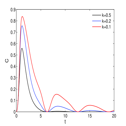
Figure 3: The time evolution of the entanglement when considering cavity decay with $g_{eff}$=1, $\alpha=1$, $\beta=1.5$. From top to bottom, $k=0.1,0.2,0.5$, respectively.

Fig.3 displays the entanglement of two cavity modes measured by concurrence for $k=0.1,0.2,0.5$, respectively. It is observed that amplitude of concurrence decreases with the increasing of $k$. The loss of the cavity destroys the entanglement. Thus, a high-Q two-mode cavity is preferred.

Furthermore, our method can also be extended to generate multidimensional entangled coherent state. In order to do this, we first send a two-level atom with a virtual intermediate level Hybrid-30 , initially in the ground state $|g\rangle$, through a two-mode cavity. The atom dispersively interact with one of the cavity mode(e.g.,cavity mode with annihilation (creation) operators $a_{1}(a_{1}^{\dagger}))$ where the two-photon process takes place. The effective Hamiltonian acting on state $|g\rangle$ is $H=-\hbar\lambda a_{1}^{\dagger}a_{1}(a_{1}^{\dagger}a_{1}-1)$ Hybrid-31 . If the cavity mode is initially in a coherent state, the nonlinear Hamiltonian interaction equals to that of the Kerr medium Hybrid-28 . When the two-level atom flies out of the cavity, a three-level atom in $\Lambda$ configuration is sent into it. Doing the same operation we discussed in section II, finally we recognize that the total evolution operator of the field part has the same form as Eq.(4) in Ref. Hybrid-28 . Following the methods of Ref. Hybrid-28 , we can derive the multidimensional entangled coherent state after a projective measurement of atomic state in the basis $\{|\pm\rangle\}$.

.4 IV. Conclusion

In conclusion, we present a scheme to generate two-mode entangled coherent state via the QED system, in which a three-level $"\Lambda"$ configuration atom interacts with two cavity modes and two classic fields in large detuning. When we perform a measurement on the atomic state, the two-mode field will collapse into the entangled coherent state if the two cavity modes are both in the coherent states initially. In our scheme the two cavity modes interact with two distinct atomic transitions, so they are easy to be controlled. Moreover, taking into account the cavity decay, we study the system evolution and give an analytical solution. With the assistance of another two-level atom with intermediate level, our scheme can also be generalized to generate multidimensional entangled coherent state.

References

• (1) Bell J S 1965 Physics (Long Island City, N.Y.) 1 195
• (2) Ekert A and Jozsa R 1996 Rev. Mod. Phys. 68 733 Knill E, Laflamme R and Milburn G J 2001 Nature 46 409
• (3) Bennett C H, Brassard G, Crepeau C, Jozsa R, Peres A and Wooters W K 1993 Phys. Rev. Lett. 70 1895 Wang X 2001 Phys. Rev. A 64 022302
• (4) Munro W J, Milburn G J and Sanders B C 2000 Phys. Rev. A 62 052108 van Enk S J and Hirota O 2001 Phys. Rev. A 64 022313 Nguyen Ba An 2004 Phys. Rev. A 69 022315
• (5) Sanders B C 1992 Phys. Rev. A 45 6811
• (6) Wielinga B and Sanders B C 1993 J. Mod. Optics 40 1923
• (7) Gerry C C 1997 Phys. Rev. A 55 2478 Zou Xu Bo, Pahlke K and Mathis W 2002 Phys. Rev. A 65 064303 Paternostro M, Kim M S and Ham B S 2003 Phys. Rev. A 67 023811 Zheng S B 2004 Phys. Rev.A 69 055801
• (8) Davidovich L, Brune M, Raimond J M and Haroche S 1996 Phys. Rev. A 53 1295
• (9) Guo G C and Zheng S B 1996 Opt. Commun. 133 142
• (10) Wang B and Duan L M 2005 Phys. Rev. A 72 022320
• (11) Solano E, Agarwal G S and Walther H 2003 Phys. Rev. lett. 90 027903
• (12) Lougovski P, Solano E and Walther H 2005 Phys. Rev. A 71 013811
• (13) Biswas A and Agarwal G S 2004 Phys. Rev. A 69 062306
• (14) Gerry C C and Grobe R 1997 J. Mod. Optics 44 41
• (15) Lu H X, Yang J, Zhang Y D and Chen Z B 2003 Phys. Rev. A 67 024101
• (16) Chai C L 1992 Phys. Rev. A 46 7187
• (17) Wang X 2002 J. Phys. A 35 165
• (18) Shchukin E and Vogel W 2005 Phys. Rev. Lett. 95 230502
• (19) Hillery M and Zubairy M S 2006 Phys. Rev. Lett. 96 050503
• (20) Zhou L, Xiong H and Zubairy M S will be published.
• (21) Peixoto de Faria J G and Nemes M C 1999 Phys. Rev. A 59 3918
• (22) Fang M F and Liu X 1996 Phys. Lett. A 210 11
• (23) Zhou L, Song H S, Luo Y X and Li C 2001 Phys. lett. A 284 156
• (24) van Enk S J 2003 Phys. Rev. Lett. 91 017902