Furnishing the Galaxy with Pulsars

Abstract

The majority of pulsar population synthesis studies performed to date have focused on isolated pulsar evolution. Those that have incorporated pulsar evolution within binary systems have tended to either treat binary evolution poorly of evolve the pulsar population in an ad-hoc manner. Here we present the first model of the Galactic field pulsar population that includes a comprehensive treatment of both binary and pulsar evolution. Synthetic observational surveys mimicking a variety of radio telescopes are then performed on this population. As such, a complete and direct comparison of model data with observations of the pulsar population within the Galactic disk is now possible. The tool used for completing this work is a code comprised of three components: stellar/binary evolution, Galactic kinematics and survey selection effects. Here we give a brief overview of the method and assumptions involved with each component. Some preliminary results are also presented as well as plans for future applications of the code.

1 Population synthesis

We evolve n systems by first selecting the initial parameters of each single star (mass) or binary (masses, period) from appropriate distributions, e.g.- stellar masses drawn from the Kroupa, Tout & Gilmore (1993) initial mass function. Limits must also be chosen where we typically take $5-80M_{\odot}$ and $0.1-40M_{\odot}$ for the binary primary and secondary masses. The algorithm loops over the n systems in binpop which follows the stellar/binary evolution. Any systems of interest that are produced (in this case pulsars) are passed to binkin which follows the kinematic evolution of each system. The resulting population is then ‘surveyed’ in binsfx which produces synthetic data for analysis.

2 binpop: Binary and Pulsar evolution

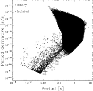
This component evolves single and binary stars from the zero age main sequence through to some given time, $t_{max}$. It uses the binary evolution code of Hurley, Tout & Pols (2002) with the addition of pulsar evolution. Some features included in the binary evolutionary algorithm are tides, mass transfer (examples are stellar winds, roche-lobe overflow and common envelope), magnetic braking, orbital gravitational radiation, mergers and supernova velocity kicks. Features particular to neutron star (NS) include, standard pulsar magnetic field decay, accretion induced field decay and spin-up, magnetic braking, propeller effects and death lines. In this body of work we focus on a particular model which makes the following assumptions and produced the pulsars shown in Figure 1. The model evolves n $=10^{7}$ binary systems, where each system is evolved to a $t_{max}$ drawn at random from between the limits of 0 and 10 Gyr. If a NS forms it’s initial spin period $P_{0}$ and magnetic field $B_{0}$ are given by $P_{0}=0.02+0.156(V_{kick}/V_{\sigma})$ [s] and $B_{0}=5x10^{11}+4x10^{12}\times(V_{kick}/V_{\sigma})$ [G], where $V_{kick}$ is randomly drawn from a Maxwellian with standard deviation $V_{\sigma}=190$ km/s. In terms of NS magnetic field decay we assumed the standard decay time constant , $\tau_{B}=1000$ Myr while the accretion induced decay scaling parameter is, $k=7000$. We then ignore pulsars whose magnetic field decays to the limiting value of $5\times 10^{7}$ G. If a NS is accreting we assume it is not visible as a pulsar and it is ignored, this includes those NS who were accreting material via Roche-lobe overflow within the previous 1000 years. Finally, this model also includes the Harding, Muslimov & Zhang (2002) curvature radiation death line, beyond which pulsars are assumed not to emit beamed emission of sufficient strength to be observed.

Figure 1: Spin period against spin period derivative for each pulsar produced in the model described to the left. Each point is one pulsar, circles represent binary pulsars while stars are isolated pulsars.

3 binkin: Galactic kinematics

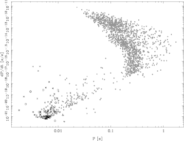
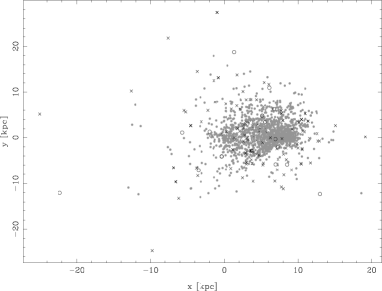
In this component single stars and binary stars are evolved dynamically within the Galactic gravitational potential, which we model as given by Kuijken & Gilmore (1989). This is our first and simplest model of the Galaxy and includes the disk, nucleus and bulge. Binkin also takes into account supernovae, which may impart some momentum onto a single star or binary system or, in fact, disrupt a binary system. Every system has it’s orientation randomised with respect to the galactic plane. The code has been tested and is reversible. We note that this is not an n-body code, each system is evolved independently. Each of the pulsars in Figure 2 & 3 are evolved in binkin which moves them in the Galaxy to produce an 3-dimensional spatial distribution. In this model the stars are assumed to be born in a disk with a radius of 15 kpc and a height above the plane of 50pc.

4 binsfx: Synthetic surveys

We now consider the final component of our work, binsfx, which uses both the pulsar data from binpop and the Galactic positional data from binkin to produce synthetic surveys. These synthetic surveys are based on the Parkes Multibeam (PMB), Swinburne intermediate latitude (SIL) and Swinburne extended (SE) surveys along with the Burgay et al. (Betal) survey. We also make use of the GMRT, which has not yet been used for an extended and large pulsar survey project. In modeling the surveys it is important that we also take into account the associated pulsar selection effects. Within the model presented here (Figures 2 & 3) we have considered beaming of the pulses away from our line of sight, scattering of the image (multi-path propagation), dispersion (a lag between different wavelengths) and sampling of the pulse with a finite time constant. We also need to assume some form of the pulsar luminosity and we do this using, $L=0.1\times 10^{0.1\chi}\times P^{\alpha}\times\frac{dp}{dt}^{\beta}$ where $\alpha=-2.0+0.1\chi$, $\beta=0.0+0.1\chi$ and $\chi$ is a Gaussian random number. We assume a spectral index of the form $-0.8\chi$. Once we check whether each pulsar produced above (depicted by Figure 1) is within the correct region of the Galaxy for the particular survey and is close enough that our assumed telescope sensitivity is less than the calculated pulsar luminosity (at the solar system) then we may start to produce plots like Figures 2 & 3. Note that Figure 2 is a reproduction of Figure 1 after passing the population through binkin and binsfx. We may now compare these to the observations. For our simulated surveys of PMB, SIL, SE and Betal we find 1180, 105, 54 and 99 pulsars respectively. With the above assumptions we predict that the GMRT could see 366 pulsars.

Figure 2: Synthetically observed pulsars from the Galactic pulsar population shown Figure 1. Each point is one pulsar, crosses are isolated millisecond pulsars while circles are binary millisecond pulsars.

Figure 3: The Galactic x-y positions of those synthetically observed pulsars shown in Figure 2. Each point is one pulsar, crosses are isolated millisecond pulsars while circles are binary millisecond pulsars.

5 Future work

The results shown here are a guide to what we can now achieve when modelling pulsars within the Galaxy. Being able to directly compare the results with observation, although not new, is a step forward when simulating with such detailed stellar and binary evolution codes. For example, the number of pulsars the above simulated surveys ‘see’ are obviously only estimates, however, through comparison with pulsar surveys we are now able to better constrain the complete underlying pulsar luminosity law. This work will also help in constraining binary and pulsar theory by allowing us to compare the spatial distributions of differing system types (for example see Figure 3) and the numbers and birth rates of these systems as directly compared to observations. Note that the binary evolution algorithm is not restricted to pulsars and any star/binary of interest can be investigated. This work will also help predict what next generation telescopes, such as the Square Kilometer Array, should see.

References

- (1) A. K. Harding, A. G. Muslimov, and B. Zhang, ApJ, 565, 375, (2002).
- (2) J. R. Hurley, C.A. Tout, and O. R. Pols, MNRAS 329, 897 (2002).
- (3) K. Kuijken, and G. Gilmore, MNRAS, 239, 571 (1989).
- (4) P. Kroupa, C. A. Tout, and G. Gilmore, MNRAS, 262, 545 (1993).
- (5) T. M. Tauris, and R. J. Takens, A&A, 330, 1047 (1998).