BEC “level” for measuring small forces

Abstract

We propose a device that consists of a trapped two-component phase- separated Bose-Einstein condensate to measure small forces and map weak potential energy landscapes. The resolution as well as the measurement precision of this device can be set dynamically, allowing measurements at multiple scales.

The mesoscopic quantum coherent matter systems, such as dilute gas Bose-Einstein condensates (BEC’s) and fermion superfluids, created in cold atom traps are unusually sensitive and clean many-body systems that can be isolated nearly completely from the influence of environment, and possess unusual control knobs such as the ability to vary the inter-particle interaction at will feshbach . This has lead to several suggestions for BEC-probes that would measure, for example, Casimir forces cornell-casimir , magnetic fields stamperkurn , or the earth’s rotation stringari . In this letter, we discuss the prospect of creating a mesoscopic sized BEC-object (a BEC “bubble”) that is free or nearly free - the effective potential energy experienced by the bubble’s center-of-mass position is nearly constant in space. Therefore, the bubble’s center-of-mass position becomes an ultra-sensitive measure of any weak external force on the bubble. At the same time, if the boundary region of the bubble is ‘sharp’ then its edge maps out potential energy contours with exquisite accuracy. The freely floating bubble also provides an intriguing template for probing mesoscopic quantum behavior. By crafting shallow external potentials superimposed upon the flat effective ‘bubble’ potential, experimentalists could demonstrate many-body quantum interference, observe quantum Brownian motion and study many-body quantum tunneling.

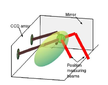
Figure 1: Schematic of the proposed BEC “level” device. The bubble of BEC-B (represented by a sphere) is confined within the BEC-A sea (shown by the ellipsoid). The arrow along the axis of the ellipsoid is the direction of the external force that causes the bubble to be displaced from the center of the ellipsoid. This displacement can be measured by a laser configuration as shown in the figure.

The actual bubble we propose to use is a trapped phase-separated BEC of ‘B’ atoms floating within a simultaneously trapped, larger BEC of ‘A’ atoms timmermans ; fermiseparation as shown in the schematic of Fig. 1. The extent of the phase separated BEC-B bubble is confined by the BEC-A sea in which it floats. By carefully choosing the trapping potentials and interaction strengths, the trapping, buoyancy, and surface tension forces on the bubble can cancel, resulting in a freely floating mesoscopic BEC object near the middle of the trap. An additional increase of the inter-species interaction strength decreases the size of the interface boundary region between the BEC’s, sharpening the ‘edge’ of the bubble. Now the bubble’s position is extraordinarily sensitive to the magnitude of a small perturbing external force. Thus, the position of the bubble becomes a measure of the magnitude of this force. Moreover, experimental methods based on imaging the shadow of the bubble as depicted in Fig. 1, can accurately measure the bubble displacement. Such techniques have proved to be yield exquisitely precise position measurements elsewhere imaging .

Conceptually, the proposed weak force detector resembles a “level” - a device that determines the horizontal direction by detecting the cancellation of the gravitational force component in the direction in which a bubble in a fluid-filled tube can move. At the point of cancellation, the bubble remains stationary in the middle of the tube. If the effective potential of the phase separated BEC bubble is exactly flat, then the actual ground state of the system is a superposition of states in which the bubble is located in different positions. If the bubble behaves as a macroscopic object, then once its position is measured, it remains localized, ‘pinned’ by interactions with the environment - an essential ingredient of the breaking of translational symmetry. If the environment interactions are sufficiently weak and in the presence of a shallow double well potential, the bubble can behave as a quantum object, tunneling between the wells (the bubble’s surface tension may prevent single particle tunneling) or interfering with itself if it can follow different paths to reach the same final position. Such experiments that reveal the quantum properties of the ‘bubble’ can be carried out on a ‘chip’ chip (near a surface). The main source of decoherence would be the excitation of phonon modes in the surrounding BEC-sea.

For the discussion in this letter, we won’t require the extreme level of control necessary for the observation of mesoscopic quantum behavior. Instead, we assume that external interactions are present (though small) and that the BEC ‘bubble’ acts as a classical object. Even in that case, the bubbles can probe genuine quantum effects, for example, the position of two bubbles each trapped in one well of a double well potential would be modified from their equilibrium position if they experience a mutual attraction, induced by Casimir-like force arising from quantum fluctuations of the surrounding BEC roberts .

We illustrate the cancellation of bubble forces in the case of a ’small bubble of vanishing surface tension’ - the simplest limit. In that case, the size of the bubble is sufficiently large to neglect the surface energy, but remains small compared to the length scale on which the trapping potentials $V_{A}({\bf r})$ and $V_{B}({\bf r})$ experienced by the ‘A’ and ‘B’ atoms respectively, vary. Hence, we can replace $V_{B}({\bf r})\approx V_{B}({\bf R})$ where ${\bf R}$ denotes the bubble’s center-of-mass position. We also assume that the BEC gas is dilute and that we can describe the inter-particle interactions by the customary contact potentials: $v_{A(B)}({\bf r}-{\bf r}^{\prime})=\lambda_{A(B)}\delta({\bf r}-{\bf r}^{\prime})$ for the mutual interactions of like bosons ‘A’ (or ‘B’) and $v_{AB}({\bf r}-{\bf x})=\lambda\delta({\bf r}-{\bf x})$ for the mutual interactions of unlike bosons. In a three-dimensional BEC gas, the contact interactions lead to local pressures within the single condensate regions of average density $\rho_{A(B)}({\bf r})$ equal to $[\lambda_{A(B)}/2]\rho_{A(B)}^{2}({\bf r})$. If we neglect the surface tension of the bubble, then the condition of equilibrium requires the inside and outside bubble pressures to cancel, i.e. $P=\lambda_{A}[\overline{\rho}_{A}({\bf R})]^{2}/2=\lambda_{B}[\rho_{B}({\bf R})]^{2}/2$, where $\overline{\rho}_{A}$ denotes the density of an all ‘A’ BEC of the same chemical potential as the actual ‘A’ BEC which surrounds the B-bubble. Hence, the inside ‘bubble’ density is equal to $\rho_{B}({\bf R})=\sqrt{\lambda_{A}/\lambda_{B}}\overline{\rho}_{A}({\bf R})$. We write the ground state energy of the trapped BEC ‘A’ which has the ‘B’ bubble of $N_{B}$ particles immersed as the energy $\overline{E}_{A}$ of the all ‘A’ BEC that has the same chemical potential as the one with the bubble, and an integral over the ‘B’ bubble volume $\Omega_{B}$ centered on ${\bf R}$. Consistent with the assumption of slowly varying trapping potentials and the neglect of the bubble surface energy, we approximate the energy densities as $V_{A(B)}({\bf r})\rho_{A(B)}({\bf r})+[\lambda_{A(B)}/2]\rho_{A(B)}^{2}({\bf r})$ and we obtain

$$E = \overline{E}_{A}+\int_{\Omega_{B}}\left[V_{B}({\bf r})\rho_{B}({\bf r})+\lambda_{B}\rho_{B}^{2}({\bf r})/2\right]$$

$$\;\;\;\;\;-\left[V_{A}({\bf r})\overline{\rho}_{A}({\bf r})+\lambda_{A}\overline{\rho}_{A}^{2}({\bf r})/2\right]d{\bf r}$$

$$\approx \overline{E}_{A}+N_{B}\left[V_{B}({\bf R})-\sqrt{\lambda_{A}/\lambda_{B}}V_{B}({\bf R})\right]\;\;,$$

consistent with an effective potential energy per B-particle equal to $V_{\text{eff},B}({\bf R})=V_{B}({\bf R})-\sqrt{\lambda_{B}/\lambda_{A}}V_{A}({\bf R})$. Now, if the trapping potentials for A and B particles are simply proportional, $V_{A}({\bf r})=\alpha V_{B}({\bf r})$, and we carefully tune the proportionality constant $\alpha$ to $\alpha\rightarrow\sqrt{\lambda_{A}/\lambda_{B}}$ then the effective potential as seen by the bubble vanishes and it floats freely inside the BEC-A.

This value, $\alpha=\sqrt{\lambda_{A}/\lambda_{B}}$ is also the proportionality constant at which the bubble’s position becomes highly sensitive to any small additional external force. We illustrate this for the case of a harmonic trapping potentials, $V_{B,\text{trap}}({\bf r})=(1/2)\left[K_{x}x^{2}+K_{y}y^{2}+K_{z}z^{2}\right]$, $V_{A,\text{trap}}({\bf r})=\alpha V_{B,\text{trap}}({\bf r})$, to which a differential external force ${\bf F}=\gamma\hat{z}$ (i.e. difference of force experienced by the A- and B- atoms) adds an approximately linear term to the B-potential $V_{B}({\bf r})=V_{B,\text{trap}}({\bf r})-\gamma z$, so that

$$V_{\text{eff},B}({\bf r}) = \left(1-\alpha\sqrt{\lambda_{B}/\lambda_{A}}\right)V_{B,\text{trap}}-\gamma z$$ (2)

$$= [(1-\alpha\sqrt{\lambda_{B}/\lambda_{A}})/2]\times$$

$$\left[K_{x}x^{2}+K_{y}y^{2}+K_{z}(z-\Delta)^{2}-K_{z}\Delta^{2}\right]\;\;,$$

centered around a position that is displaced along the $z$-axis from the former trap middle by a distance $\Delta=\gamma[K_{z}\left(1-\alpha\sqrt{\lambda_{B}/\lambda_{A}}\right)]^{-1}$. Hence, in equilibrium, the measurement $\Delta$ provides a direct measurement of the magnitude of the force, $|{\bf F}|=\gamma$.

The accuracy with which the bubble’s position can be measured depends on the sharpness of its edge. In the edge region if we assume the respective BEC densities to vary as $\rho_{B}(\epsilon)=\rho_{B}({\bf R})(\delta-\epsilon)/\delta$ and $\rho_{A}(\epsilon)=\rho_{A}({\bf R})\epsilon/\delta$, where $0\leq\epsilon\leq\delta$ is normal to the interface area ${\mathcal{A}}$, then the resulting kinetic energy contribution can be approximated by $E_{\text{kin},\delta}=4{\mathcal{A}}P[l_{A}^{2}+l_{B}^{2}]/\delta$, where $l_{A(B)}=\hbar/\sqrt{4m_{A(B)}n_{A(B)}\lambda_{A(B)}}$ is the coherence length of BEC-A(B). We also find the surface interaction energy to be approximately equal to $E_{\text{int},\delta}={\mathcal{A}}P(\lambda-\sqrt{\lambda_{A}\lambda_{B}})\delta/3$. Thus the equilibrium ‘edge’ width obtained by minimizing this additional surface energy $E_{\text{edge}}=E_{\text{kin},\delta}+E_{\text{int},\delta}$ is given by $\overline{\delta}=\sqrt{12(l_{A}^{2}+l_{B}^{2})/(\lambda/\sqrt{\lambda_{A}\lambda_{B}}-1})$ timmermans . Therefore the ‘edge’ sharpness can be increased by increasing the interaction strength between unlike bosons by means of an interspecies scattering resonance interspeciesfeshbach . This increases the importance of the surface energy, requiring either a description that includes surface tension explicitly, or a numerical solution of the coupled Gross-Pitaevskii (GP) like equations. Given the lack of space, we choose the latter option and solve the numerical equations by evolving the GP-dynamics in imaginary time. Motivated by recent experiments with elongated BEC’s schmiedmayer created by focusing a singe laser beam, we consider a quasi-1D configuration with $\omega_{z}$ and $\omega_{\perp}$, the trapping frequency in the axial and transverse direction respectively, and $\xi=\omega_{z}/\omega_{\perp}<<1$ for both species of bosons.

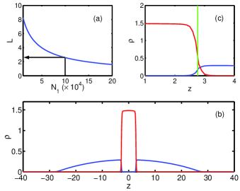
Figure 2: Figure comparing an analytical calculation that neglects the surface tension and the numerical GP solution. In (a) the half axial length, $L$, of the bubble is plotted as a function of $N_{1}$ for $N_{2}=2\times 10^{4}$, $\alpha=0.9$, $\xi=0.01$, $\beta=0.9$, and $a_{1}=0.001$, (b) the density profile obtained numerically for $N_{1}=10^{5}$ is shown, and (c) shows the magnified view of the interface region in (b). The green line indicates the boundary between BEC-A and -B obtained in (a).

The wavefunctions, $\phi_{A}$ and $\phi_{B}$ of the two interacting condensates evolve according to the coupled Gross-Pitaevskii (GP) equations

$$i\dot{\phi}_{A(B)}=\Big{[}\frac{-\nabla^{2}}{2}-\mu_{A(B)}+V_{A(B)}({\bf r})\hskip 71.13188pt$$

$$+\lambda_{A(B)}N_{A(B)}|\phi_{A(B)}|^{2}\Big{]}\phi_{A(B)}+\lambda N_{B(A)}|\phi_{B(A)}|^{2}\phi_{A(B)}$$

where the mass of ‘A’ and ‘B’ atoms is assumed to be same, $V_{A}({\bf r})=\alpha V_{B}({\bf r})=\alpha(x^{2}/2\xi^{2}+y^{2}/2\xi^{2}+z^{2}/2)$, all the physical quantities are scaled in axial harmonic oscillator units, and the condensate wavefunctions $\phi_{A(B)}$ are normalized to unity. We work in the phase separated regime by using $\lambda/\sqrt{\lambda_{A}\lambda_{B}}=1.1$. The density profile obtained numerically is plotted in Fig. 2. In the same figure we also plot the value of the half axial length, $L$, obtained by neglecting surface tension and taking the Thomas-Fermi approximation. For treating the quasi-1D situation considered here, we use a modified local density ansatz given by $\mu_{A(B)}(z)=\mu_{A(B)}-V_{A(B)}(z)$ and $\mu_{A(B)}(z)=\sqrt{\alpha/\xi^{2}}\sqrt{1+4a_{A(B)}\rho_{A(B)}(z)}$ where $a_{A(B)}$ is the two-body $s$-wave scattering length for atoms ‘A’(‘B’) gerbier which determines the interaction strength by the relation $\lambda_{A(B)}=4\pi\hbar^{2}a_{A(B)}/m$. Figure 2.(c) shows excellent agreement between $L$ and the numerically obtained location of the bubble edge.

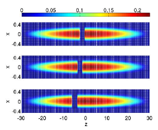
Figure 3: Density of BEC-A is shown as a surface plot for $\gamma=0.1$. The subplots top, middle, and bottom correspond to $\alpha\sqrt{\lambda_{B}/\lambda_{A}}=0.90,0.93$ and $0.95$ respectively. The BEC-B bubble is located within BEC-A where $\rho_{A}({\bf r})=0$.

We demonstrate the working of the BEC “level” by considering an external force in the axial direction ${\bf F}=\gamma\hat{z}$. As argued before, we tune the inter-atomic interactions such that $\alpha\sqrt{\lambda_{B}/\lambda_{A}}\rightarrow 1^{-}$ and $\lambda>\sqrt{\lambda_{A}\lambda_{B}}$. The corresponding ground state density profile obtained numerically is shown in Fig. 3. Here we see that the BEC-B bubble is displaced from the center of the trap by a distance $\Delta\approx\gamma/(1-\alpha\sqrt{\lambda_{B}/\lambda_{A}})$. The boson-boson interaction strength as well as the trapping frequencies can be precisely tuned in current cold-atom experimental setups resulting in a large displacement of the bubble and thus allowing for the precise measurement of $|{\bf F}|=\gamma$.

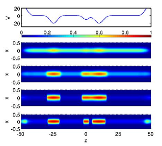
Figure 4: Density profile of the quasi-1D BEC-B for different values of $N_{A}$. The topmost figure shows the trapping potential while the remaining four plots (from top to bottom) correspond to $N_{A}=0,1000,1500,2000$.

While the above discussion was related to determining the force (gradient of the external potential), the proposed BEC “level” can also be used for mapping accurate potential energy contours. In fact such a measurement can be achieved using a single BEC as demonstrated in schmiedmayer . This experiment related the observed BEC-density profile to the variation of the external potential. The experimental accuracy of the potential was a few Hz with a spatial resolution of few microns. One limitation of the potential measurement is set by the magnitude of the chemical potential. One cannot arbitrarily decrease the chemical potential or the density of the BEC will drop below what is necessary for imaging the atoms or, if the inter-particle interaction is lowered, the coherence length of the BEC will increase to limit the spatial resolution. In contrast, the phase separated BEC configuration discussed in the present letter not only ensures large density inside the bubble allowing good imaging, but an edge width that can be reduced below typical BEC-coherence lengths allowing increased spatial resolution. We demonstrate this principle by considering an axially varying potential $V_{\text{trap}}(z)$ as shown in the topmost subplot of Fig. 4. In the same figure, the remaining subplots, show the density profile of the BEC-B as a function of the total number of ‘A’ atoms, $N_{A}$. Here we see that as $N_{A}$ is increased, the equilibrium size of the BEC-B bubble decreases. This continues till a point is reached when the BEC-B bubble is small enough and is localized in the valleys of the potential landscape. Moreover, as mentioned earlier, the edge sharpness can be improved by modifying the inter-species interaction strength $\lambda$. Thus we see that the proposed BEC “level” device can map potential energy contours arising from, for example, surface magnetic fields with exquisite precision.

In conclusion, we proposed a device for measuring small forces (gradient of potential) by using a phase separated two component BEC configuration. The working of this device is analogous to that of a level, so that we named it a “BEC-level”. This device can also map out potential energy contours with exquisite accuracy. This device could, for instance, map potential energy variations experienced by atoms near the surface of a metal caused by fluctuations of the surface fields. The BEC-level provides several knobs that can be tuned, allowing for measurements to be carried out at multiple levels of accuracy.

While we have only exploited the bubble as a classical object, its possible range of explorations includes mesoscopic quantum behaviour such as many-body tunneling, quantum interference, and quantum Brownian motion. Along with the device proposed in this letter, the BEC-level can be used as a template for probing quantum many-body behaviour.

S.B acknowledges financial support from the W. M. Keck Program in Quantum Materials at Rice University. E.T. acknowledges support from the laboratory directed research and development (LDRD) program.

References

- (1) C. Chin et al., Science, 305, 1128 (2004); C. A. Regal, M. Greiner, and D. S. Jin, Phys. Rev. Lett. 92, 040403 (2004); M. W. Zwierlein et al., cond-mat/0403049 (2004); T. Bourdel et al., Phys. Rev. Lett. 93, 050401 (2004); K.M. O’ Hara et al., Science 298, 2179 (2002); R. Hulet, presentation in the Quantum Gas Conference at the Kavli Institute for Theoretical Physics, Santa Barbara, CA, May 10-14 (2004).
- (2) J. M. Obrecht, R. J. Wild, M. Antezza, L. P. Pitaevskii, S. Stringari, and E. A. Cornell, Phys. Rev. Lett. 98, 063201 (2007).
- (3) M. Vengalattore, J. M. Higbie, S. R. Leslie, J. Guzman, L. E. Sadler, and D. M. Stamper-Kurn, Phys. Rev. Lett. 98, 200801 (2007).
- (4) S. Stringari, Phys. Rev. Lett. 86, 4725 (2001).
- (5) Eddy Timmermans, cond-mat/9709301 ; Eddy Timmermans, Phys. Rev. Lett. 81, 5718 (1998); J. Stenger, S. Inouye, D. M. Stamper-Kurn, H. -J. Miesner, A. P. Chikkatur, and W. Ketterle, Nature 396, 345 (1998); D. S. Hall, M. R. Matthews, J. R. Ensher, C. E. Wieman, and E. A. Cornell, Phys. Rev. Lett. 81, 1539 (1998) .
- (6) Such phase separation occurs in trapped Fermi-gas systems as well: G. B. Partridge, W. Li, R. I. Kamar, Yean-an Liao, and R. G. Hulet, Science 311, 503 (2006); T. N. De Silva and E. J. Mueller, Phys. Rev. A 73 051602 (2006); K. B. Gubbels, M. W. J. Romans, and H. T. C. Stoof, Phys. Rev. Lett. 97, 210402 (2006).
- (7) S. Schneider, A. Kasper, Ch. vom Hagen, M. Bartenstein, B. Engeser, T. Schumm, I. Bar-Joseph, R. Folman, L. Feenstra, and J. Schmiedmayer, Phys. Rev. A 67 023612 (2003), D. M. Harber, J. M. Obrecht, J. M. McGuirk, and E. A. Cornell, Phys. Rev. A 72, 033610 (2005).
- (8) S. Aubin, S. Myrskog, M. H. T. Extavour, L. J. Leblanc, D. Mckay, A. Stummer, and J. H. Thywissen, Nature 2, 384 (2006); Ying-Ju Wang, D. Z. Anderson, V. M. Bright, E. A. Cornell, Q. Diot, T. Kishimoto, M. Prentiss, M. Saravanan, S. R. Segal, and S. Wu, Phys. Rev. Lett. 94, 090405 (2005); Y. Shin, C. Sanner, G. -B. Jo, T. A. Pasquini, M. Saba, W. Ketterle, D. E. Pritchard, M. Vengalattore, and M. Prentiss, Phys. Rev. A 72 021604 (2005).
- (9) D. C. Roberts and Y. Pomeau, Phys. Rev. Lett. 95, 145303 (2005).
- (10) M. Zaccanti, C. D’Errico, F. Ferlaino, G. Roati, M. Inguscio, and G. Modugno, Phys. Rev. A 74, 041605 (2006); and references therein.
- (11) F. Gerbier, Europhys. Lett. 66, 771 (2004).
- (12) P. Krüger, S. Wildermuth, S. Hofferberth,M. Andersson, S. Groth, I. Bar-Joseph, and J. Schmiedmayer, J. Phys. 19, 56 (2005).