Combining astrometry with the light-time effect:
The case of VW Cep, $\zeta$ Phe and HT Vir.

Abstract

Three eclipsing binary systems with astrometric orbit have been studied. For a detailed analysis two circular-orbit binaries (VW Cep and HT Vir) and one binary with an eccentric orbit ($\zeta$ Phe) have been chosen. Merging together astrometry and the analysis of the times of minima, one is able to describe the orbit of such a system completely. The $O-C$ diagrams and the astrometric orbits of the third bodies were analysed simultaneously for these three systems by the least-squares method. The introduced algorithm is useful and powerful, but also time consuming, due to many parameters which one is trying to derive. The new orbits for the third bodies in these systems were found with periods $30$, $221$, and $261$ yr, and eccentricities $0.63$, $0.37$, and $0.64$ for VW Cep, $\zeta$ Phe, and HT Vir, respectively. Also an independent approach to compute the distances to these systems was used. The use of this algorithm to VW Cep gave the distance $d=(27.90~{}\pm~{}0.29)~{}\mathrm{pc}$, which is in excellent agreement with the previous Hipparcos result.

1 Introduction

During the last century, many observations of close binary systems were collected, especially for eclipsing binaries. Most observations of these stars were made photometrically but in some cases also the spectroscopy was obtained. In a few cases, also astrometric observations were carried out and these systems, which were studied by several different techniques, are the most interesting, because one is able to find more relevant parameters of them. Especially, if it is possible to analyse the different measurements together (it means from different observational techniques in one least-squares fit) one is able to find the complete set of parameters describing the orbit of such a binary, which are not in contradiction. Such approach is potentially very powerful, especially in upcoming astrometric and photometric space missions.

There are a few well-known eclipsing binaries with astrometric measurements for which the light-time effect (hereafter LITE) was considered, or expected. However, the eclipsing binary (hereafter EB) nature and the astrometric orbit were usually studied separately.

For example, there are several published light-curve solutions for V505 Sgr with the third light included (see e.g. Lázaro et al. (2006), İbanoǧlu et al. (2000), etc), and an analysis of its apparent orbital period changes interpreted as the LITE due to the third body (e.g. Rovithis-Livaniou et al. 1991). The only paper which compares the astrometry and a period analysis of $O-C$ deviations from the constant orbital period was published by Mayer (1997). Despite existing astrometric measurements, there were no attempts to combine these two methods together. The results from different approaches were just compared to each other.

Another systems are for instance  QS Aql,  44i Boo,  QZ Car, SZ Cam, GT Mus, or V2388 Oph. The coverage of the astrometric orbit is very poor for some of them. In the system QS Aql the LITE could be determined precisely, but the astrometric orbit is covered only very poorly, see e.g. Mayer (2004). The opposite case is V2388 Oph, where the astrometric-orbit parameters were computed very precisely, but there are only a few minimum-time measurements (see e.g. Yakut et al. 2004). For SZ Cam only a few usable astrometric observations were obtained, but the LITE is well-defined and also the third light in the light-curve solution was detected (Lorenz et al. 1998). QZ Car is a more complicated, probably quadruple system consisting of an eclipsing and a non-eclipsing binary, but there are also only a few usable astrometric measurements. Also GT Mus is a quadruple system, consisting of an eclipsing and RS CVn component. In many other cases, only measurements of the times of minima are available, without astrometry. For some others, astrometry without photometry, is only available. Other systems where the astrometric observations were obtained and the LITE is observable or expected are listed in Mayer (2004).

The only paper on combining these two different approaches into one joint solution is that by Ribas et al. (2002), where a similar method as described in this paper was applied to the system R CMa, but where only a small arc of the astrometric orbit was available. Besides the astrometry and LITE also the proper motion on the long orbit was analyzed. On the other hand one has to note, that in Ribas et al. (2002) the complete astrometric parameters (with proper motions, parallax, etc.) were used, while in this paper only a relative astrometry of the distant body relative to the eclipsing pair was analysed.

2 Methods

2.1 Astrometry

The number of visual binaries with astrometric orbits has grown, but the whole orbit is covered with data points only in some cases. Thanks to precise interferometry the observable semimajor axes of astrometric binaries are still decreasing down to milli- and micro-arcseconds.On the other hand, one has to regret that no recent astrometric measurement of a wide pair of about 1^′′  has been obtained for the systems mentioned below.   All the astrometric observations were adopted from ’The Washington Double Star Catalogue’ WDS (Mason et al. 2001).

From astrometric data ($N$ measurements of the position angle $\theta_{i}$, separation $\rho_{i}$, the uncertainties $\sigma_{\theta}$, and $\sigma_{\rho}$ and the time of the observation $t_{i}$) one is trying to find out the parameters of the orbit for the distant component, defined by 7 parameters: period $p_{3}$, angular semimajor axis $a$, inclination $i$, eccentricity $e$, longitude of the periastron $\omega_{3}$, the longitude of the ascending node $\Omega$, and the time of the periastron passage $T_{0}$. One has to solve the inverse problem

$$\{(t_{i},\theta_{i},\rho_{i},\sigma_{\theta,i},\sigma_{\rho,i})\}_{i=1,N}\rightarrow(a,p_{3},i,e,\omega_{3},\Omega,T_{0}).$$

The least-squares method and the simplex algorithm was used (see e.g. Kallrath & Linnell 1987).

Comparing the theoretical position on the sky $\theta_{0}$ and $\rho_{0}$ with the observed ones $\theta_{i}$ and $\rho_{i}$, one can calculate the sum of normalized residuals squared

$${\chi^{2}_{astr}}=\sum_{i=1}^{N}\left[\left(\frac{\theta_{i}-\theta_{0,i}}{\sigma_{\theta,i}}\right)^{2}+\left(\frac{\rho_{i}-\rho_{0,i}}{\sigma_{\rho,i}}\right)^{2}\right],$$ (1)

following Torres (2004). With this $\chi^{2}_{astr}$ and using the simplex algorithm one can obtain a set of parameters ($a$, $p_{3}$, $i$, $e$, $\omega_{3}$, $\Omega$, $T_{0}$) describing the astrometric orbit.

The weighting is provided by the uncertainties $\sigma_{\theta}$ and $\sigma_{\rho}$. These values are obtained from the observations, or estimated as some typical uncertainty level for the certain kind of measurement provided by a specific instrument.

The efficiency and the computing time required by the algorithm strongly depends on the initial set of parameters and the chosen trial step in the parameter space. If nothing is known about the solution, one has to scan a wide range of parameters (eccentricity $e$ from $0$ to $1$, and the angular parameters from $0^{\circ}$ to $360^{\circ}$).

The efficiency of the algorithm could be improved if the simplex is used repeatedly. It can happen that the simplex converges into a local minimum while the global one is far away. It is therefore advisable to run the algorithm again, with as large initial steps as in the previous run, but keeping the values of the parameters corresponding to the previously found minimum as one vertex. Repeating this strategy several times over the whole parameter space, one can judge whether the global minimum was found by checking whether the sum of squares of the residuals is still changing or not.

To conclude, using this strategy and the combined method described in section 2.3, one gets the satisfactory result after large number of iterations. This number and computing time is strongly depended on the input data set and the number of parameters fitted. For the case VW Cep with the largest data set (about 1600 data points, see below) and also with the most parameters to fit (14 in total) one reaches the solution, when the sum of squares is not changing significantly, after circa 100,000 simplex steps. This takes about one day on computer with 2 GHz processor.

2.2 Light-time effect

A different method to study eclipsing binaries in hierarchical triple systems is based on the eclipse timings. The light-time effect (or the ’light-travel time’) causes apparent changes of the observed binary period with a period corresponding to the orbital period of the third body. This useful method is known for decades and its detailed description was presented by Irwin in 1959, while some comments on it and its limitations were discussed by Frieboes-Conde & Herczeg (1973) and by Mayer (1990).

From the numerical point of view the method is quite similar to the previous one, because it is also an inverse problem. One has $M$ measurements of the times of minima of the system at certain constant $JD_{i}$ with the individual uncertainties $\sigma_{m}$. The task is to find five parameters describing the orbit of the third body in the system: the period of the third body $p_{3}$, the semiamplitude of the LITE $A$, the eccentricity $e$, the time of the periastron passage $T_{0}$, and the longitude of periastron $\omega_{12}$. One has to compute simultaneously also two (or three) parameters of the eclipsing binary itself, namely its linear (or quadratic) ephemeris $JD_{0}$ and period $P$ (and $q$ for the quadratic one). Altogether, one has 7 (or 8) parameters to derive from the model fit of the minimum-time measurements

$$\{(JD_{i},\sigma_{m,i})\}_{i=1,M}\rightarrow(p_{3},A,e,T_{0},\omega_{12},JD_{0},P,q).$$

Similarly as in the astrometry case, the resultant sum of normalized square residuals is

$$\chi^{2}_{LITE}=\sum_{i=1}^{M}\left(\frac{(O-C)_{i}}{\sigma_{m,i}}\right)^{2},$$ (2)

where $O$ and $C$ stand for observed and computed time of minimum, respectively. The same remarks about the efficiency and the computing time required discussed for the astrometric solution also apply here.

At this place it is necessary to remark one useful comment. One has to distinguish between the two angles $\omega_{3}$ and $\omega_{12}$. The parameter used in LITE analysis is $\omega_{12}$, but in astrometry the quantity $\omega_{3}~{}=~{}\omega_{12}~{}+~{}\pi$ is employed. In this paper the angle $\omega$ stands for the longitude of the periastron for the eclipsing binary, i.e. $\omega~{}=~{}\omega_{12},$ and the subscripts will be omitted for clarity.

2.3 Combining the methods

The task is to combine the astrometry and the analysis of times of minima into one joint solution together. Having $N$ astrometric and $M$ minimum time measurements, one is able to merge them together and obtain a common set of parameters

$$(t_{i},\theta_{i},\rho_{i}, \!\!\sigma_{\theta,i} \!\!,\sigma_{\rho,i},JD_{i},\sigma_{m,i})\rightarrow$$

$$\rightarrow (a,p_{3},i,e,\omega,\Omega,T_{0},JD_{0},P,q).$$

This set of 10 parameters fully describes the orbit of the eclipsing binary around the common centre of mass with the third unresolved component together with the ephemeris of the binary itself. It is necessary to solve one least-squares fit of these 10 parameters.

One is able to find out the mass of the third body and the semimajor axis of the wide orbit because the inclination is known and one can calculate the mass function of the wide orbit

$$f(M_{3}) = \frac{(a_{12}\sin i)^{3}}{p_{3}^{2}}=\frac{(M_{3}\sin i)^{3}}{(M_{1}+M_{2}+M_{3})^{2}}=$$ (3)

$$= \frac{1}{p_{3}^{2}}\cdot{\left[\frac{173.15\cdot A}{\sqrt{1-e^{2}\cos^{2}\omega}}\right]^{3}},$$

where $a_{12}$ stands for the semimajor axis of the binary orbit around the common centre of mass and $M_{1},M_{2},M_{3}$ are the masses of the primary, secondary, and tertiary component, respectively. For more details see e.g. Mayer (1990).

The only difficulty which remains unclear is the connection between the angular semimajor axis $a$ and the amplitude of LITE $A$. The quantity $a_{12}$ could be derived from Eq. 3 and with the masses of the individual components one is able to calculate also the value $a_{3}$, i.e. the semimajor axis of the third component around the barycentre of the system

$$a_{3}=a_{12}\cdot\frac{M_{1}+M_{2}}{M_{3}}.$$ (4)

The total mutual distance of the components is $a_{\mathrm{total}}=a_{12}+a_{3}$. Using the Hipparcos parallax $\pi$ (Perryman & ESA 1997) one can obtain the distance $d$ to the system. Now it is possible to enumerate the angular semimajor axis $a$ as a function of $d$ and $a_{\mathrm{total}}$

$$a~{}=~{}\arcsin\left(\frac{a_{\mathrm{total}}}{d}\right).$$ (5)

The way how these two different approaches were putted together is following the similar approach by Torres (2004). From the mathematical point of view both methods are analogous and there is an overlap of the parameters in both methods. Our task is to minimize the combined $\chi^{2}$

$$\chi^{2}_{comb}=\chi^{2}_{astr}+\chi^{2}_{LITE},$$ (6)

where the values $\chi^{2}_{astr}$ and $\chi^{2}_{LITE}$ are taken from the Eqs.1 and 2.

Sometimes there arises a problem with the $\chi^{2}$ values in both methods, which are incomparable. Especially when there are much more data points in one method against the other, also the resultant $\chi^{2}$ would be much larger and as a consequence this method outweigh the other one. This problem could be eliminated using new uncertainties $\sigma^{\prime}$

$$\sigma_{\theta}^{\prime}=\sqrt{N}\cdot\sigma_{\theta},\,\,\,\,\sigma_{\rho}^{\prime}=\sqrt{N}\cdot\sigma_{\rho},\,\,\,\,\sigma_{m}^{\prime}=\sqrt{M}\cdot\sigma_{m}\,.$$

3 An application of the method to several particular systems

The method described above was tested on a few systems satisfying the following conditions: 1. More than 10 times of minima and more than 10 astrometric observations are available. 2. The observed range of the position angle in the astrometric measurements is larger than 10^∘.

Table 1: The final results: Parameters of the third bodies from combined astrometry and the light-time effect. The table is divided into three parts, in the first one are ten computed parameters, in the second one the values from the literature and in the last one the quantities computed from the previous parts. The values of parallax and distance were adopted from the Hipparcos measurements. In the row ’Data set’, ’a’ and ’m’ denote the number of astrometric observations, and times of minima, respectively.

Parameter	Unit	VW Cep	$\zeta$ Phe	HT Vir
$JD_{0}$	$[$HJD$]$	$2437001.4327\pm 0.0025$	$2441643.7382\pm 0.0008$	$2452722.5040\pm 0.0050$
$P$	$[$d$]$	$0.278315349\pm 0.00000012$	$1.6697772\pm 0.0000013$	$0.4076696\pm 0.0000025$
$p_{3}$	$[$yr$]$	$29.79\pm 0.08$	$220.9\pm 3.5$	$260.7\pm 0.40$
$T_{0}$	$[$HJD$]$	$2450390.6\pm 37.3$	$2419908.9\pm 2465.6$	$2442832.3\pm 60.6$
$\omega$	$[^{\circ}]$	$239.28\pm 2.88$	$97.1\pm 2.2$	$250.9\pm 0.6$
$e$		$0.633\pm 0.007$	$0.366\pm 0.082$	$0.640\pm 0.005$
$A$	$[$d$]$	$0.0131\pm 0.0004$	$0.0808\pm 0.0080$	$0.1274\pm 0.0024$
$a$	$[$mas$]$	$445.2\pm 33.0$	$859.5\pm 137.2$	$1023.5\pm 183.3$
$i$	$[^{\circ}]$	$33.6\pm 1.2$	$64.4\pm 3.0$	$45.4\pm 3.7$
$\Omega$	$[^{\circ}]$	$17.7\pm 3.1$	$33.5\pm 4.9$	$180.8\pm 2.6$
$M_{12}$	[$\mathrm{M_{\odot}}$]	$1.37$	$6.48$	$2.3$
References		Kaszas et al. 1998	Andersen 1983	D’Angelo et al. 2006
$\pi$	$[$mas$]$	$36.16\pm 0.97$	$11.66\pm 0.77$	$15.39\pm 2.72$
$d$	$[$pc$]$	$27.7\pm 0.7$	$85.8\pm 5.7$	$65.0\pm 11.5$
$a_{12}$	$[$AU$]$	$4.33\pm 0.20$	$15.52\pm 1.60$	$32.23\pm 0.74$
$f(M_{3})$	[$\mathrm{M_{\odot}}$]	$0.0154\pm 0.0016$	$0.0562\pm 0.0167$	$0.1692\pm 0.0098$
$M_{3}$	[$\mathrm{M_{\odot}}$]	$0.74\pm 0.07$	$1.73\pm 0.26$	$2.10\pm 0.10$
Data set		16a + 1594m	12a + 36m	275a + 31m

3.1 VW Cep

The eclipsing binary VW Cep (HD 197433, BD +75 752, HIP 101750, $V=7.3$ mag, sp G5V + G8V) is a W UMa system and in fact it is one of the most often observed and analysed system. Both components are chromosphericaly active. VW Cep is rather atypical, because during the primary (the deeper one) eclipse is the less massive star (the hotter one) occulted by the larger companion (the more massive and the cooler one).

The first observations of its light variations were done by Schilt (1926). Since 1946, a large amount of photoelectric observations was obtained. However, the observed minima times did not fit the ephemeris due to the LITE and the mass transfer between components. There were many light-time effect studies of this system and Herczeg & Schmidt (1960) proposed the presence of a third body with an orbital period of 29 years and an angular distance of the third component between 0.5 ^′′  and 1.2 ^′′.

In 1974, the first successful visual observation of the third component was obtained and since then, there were 16 observations of it. Regrettably, the observations near the periastron passage are missing (the gap in data is from 1991 to 1999). The last two measurements ($\theta=231.4^{\circ}$, $\rho=0.702$^′′ and $\theta=232.6^{\circ}$, $\rho=0.695$^′′) were not published yet. These were obtained by a speckle camera in April 2007 and were kindly sent by Elliot Horch (priv.comm.).

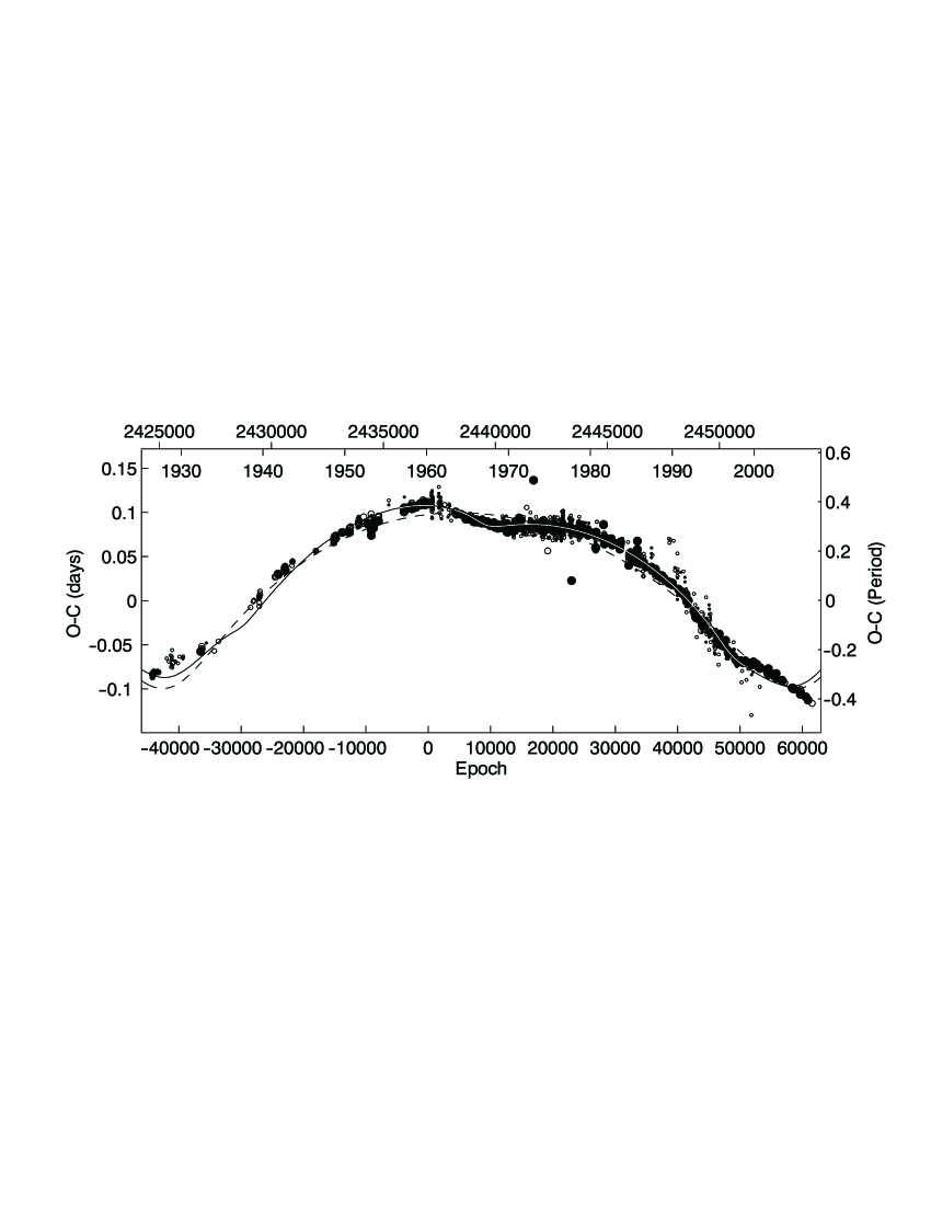
Figure 1: An $O-C$ diagram of VW Cep. The individual observations are shown as dots (primary) and open circles (secondary), the small ones for visual and the large ones for CCD and photoelectric observations. The curves represent the predicted LITE₃ + LITE₄ (the solid one) and only LITE₄ (the dashed one).

The most complete set of times of minima is in the most recent period study of VW Cep by Pribulla (2000). The first times of minima are from the 1920’s and altogether 1907 minima were collected. From this set of times of minima 313 measurements were neglected due to their large scatter (mostly the visual ones). This new minimum-time analysis is based on a larger data set (about 750 times of minima more than were used by Pribulla et al.). Two new CCD observations of the minimum light of VW Cep were obtained in Ondřejov observatory with the 65-cm telescope and Apogee AP-7 CCD camera, 2 seconds exposure time in R filter. These new times of heliocentric minima are the following: $2454154.3094~{}\pm~{}0.0001$ and $2454195.49866~{}\pm$ $\pm~{}0.00012$.

The short-term variations with the period of about two years (see e.g. Kwee 1966 and Hendry & Mochnacki 2000) are probably caused by the surface activity cycles on the primary component. Due to this activity an unique interpretation of the behaviour of period changes is still missing. Pribulla et al. proposed a mass transfer (the quadratic term) plus the third and the fourth body in the system (two periodic terms). Nevertheless, they were not able to explain the $O-C$ diagram in detail.

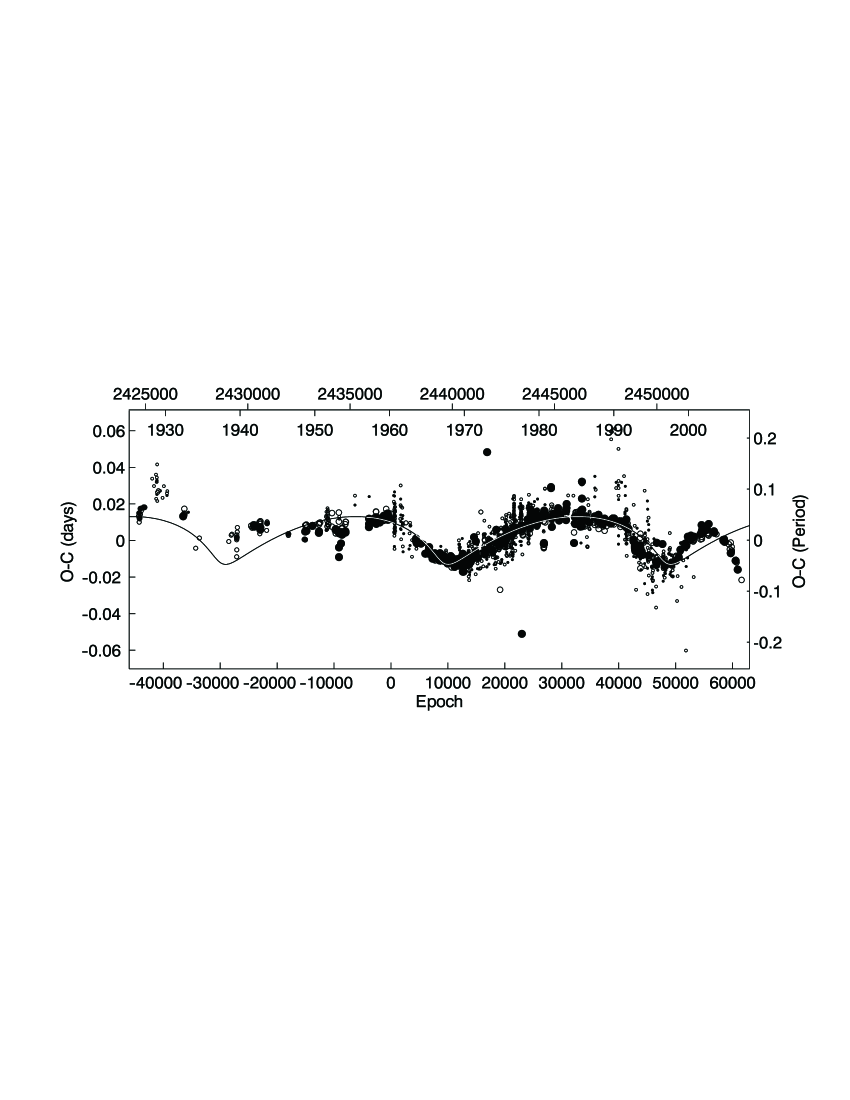
Figure 2: An $O-C$ diagram of VW Cep after subtraction of the LITE₄. The description is the same as in the previous $O~{}\!-~{}\!C$ figure, and the solid line represents the LITE caused by the third component in the system.

Another approach has been chosen in this paper. Especially due to only a few astrometric observations (16 measurements from 1974 to 2007) we have decided to explain only the most significant effects in the $O-C$ diagram. It means the astrometric variation with a period of about 30 years has been identified with the $O-C$ variation with the same period, but the long-term variation in the $O-C$ diagram (which has been interpreted by Pribulla et al. as a quadratic term) was explained as a variation due to the fourth body on its very long orbit. This approach was chosen especially because of the systemic-velocity variations, see below. It means during the computation process the value $\chi^{2}_{comb}$ was minimized with respect to 14 parameters in total:
$(A,p_{3},i,e,\omega,\Omega,T_{0},JD_{0},P,A_{4},p_{4},e_{4},\omega_{4},T_{0,4}).$

The combined approach of analysing the times of minima together with astrometry led to the parameters shown in Table 1 and 2. The $O-C$ diagram in Fig. 1 shows the times of minima together with the curve which represents the LITE₃ + LITE₄. If one subtracts only the LITE₄ variation and try to describe the behavior of the minimum times, one gets Fig. 2, where only the LITE₃ caused by the third component is displayed. The fit is not very satisfactory because of the presence of the chromospheric activity of the individual components, or due to a putative additional component (see e.g. Pribulla 2000). In Fig. 3, the astrometric orbit of the binary with the individual measurements and their theoretical positions is shown. Regrettably, no observations near the periastron passage are available. The curve also represents the theoretical orbit according to the parameters given in Table 1 in agreement with the LITE analysis.

The parameters describing the LITE₃ and LITE₄ variations are in Table 1 and 2 and could be compared to the parameters derived during the previous analysis by Pribulla et al. Their values for the third-body orbit are: $p_{3}=31.4$ yr, $e~{}=~{}0.77$, $\omega~{}=~{}183^{\circ}$, and $a_{\mathrm{total}}~{}=~{}12.53$ AU. Our values are in Table 1 except for $a_{\mathrm{total}}~{}=~{}12.35$ AU, and as we can see they differ significantly in several parameters. This is due to completely different approach describing the $O-C$ variations. Only the period and the amplitude of such variation are comparable, but these are the most important for our combined solution. One has also to disagree with the result by Pribulla et al., that the astrometric orbit could not be identified with the LITE₃ variation from the $O-C$ diagram. As one can see, our new results are in agreement with each other without any problems.

Table 2: VW Cep: parameters of the fourth-body orbit

Parameter	Unit	Value $\pm$ Error
$p_{4}$	[yr]	77.46 $\pm$ 0.04
$A_{4}$	[d]	0.100 $\pm$ 0.002
$\omega_{4}$	[∘]	283.42 $\pm$ 2.30
$T_{0,4}$	[HJD]	2453857.4 $\pm$ 13.6
$e_{4}$		0.543 $\pm$ 0.007

Also the astrometric orbit could be compared with the previously published one. Most recently Docobo & Ling (2005) published the following parameters of the astrometric orbit: $p_{3}~{}=~{}31.0$ yr, $a~{}=~{}485$ mas, $i~{}=~{}39.3^{\circ}$, and $e~{}=~{}0.68$. If one compares these values with the new ones (see Table 1), one can see that the differences are slightly beyond the limits of errors.

If we assume the mass of the eclipsing binary to be $M_{12}=1.37~{}$$\mathrm{M_{\odot}}$ (Kaszas et al. 1998) and the parallax $\pi~{}=~{}36.16~{}\mathrm{mas}$ (from Perryman & ESA 1997), the distance to the system is only about $27.66~{}\mathrm{pc}$, which results in the third-body mass of $M_{3}~{}=~{}0.741~{}$$\mathrm{M_{\odot}}$. The distant component is about 2.2 magnitudes fainter than the VW Cep itself, so its luminosity and also mass should be much smaller than the mass of the eclipsing components. The total bolometric magnitude of VW Cep is about 4.7 mag, so the magnitude of the third component is about 6.9 mag, which leads to the spectral type of about K3. The typical mass of this spectral type is about $0.75~{}$$\mathrm{M_{\odot}}$ (according to Harmanec 1988), which is in good agreement with the new result and within its error limits.

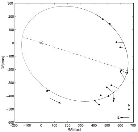
Figure 3: Relative orbit of VW Cep on a plane of the sky. The points represent individual observations, while the solid curve corresponds to the solution described in the text. The straight lines connect individual observations with their expected positions on the fitted orbit. The cross indicates the position of the eclipsing binary on the sky and the arrow the direction of the orbit of the third body. The dashed-line represents the line of apsides.

Figure 4: Systemic velocity variations in VW Cep. The individual points represent computed systemic velocities (see details in text). The solid curve stands for the combined LITE₃ + LITE₄ variations, while the dashed one only for the LITE₄ variation.

Different systemic velocities $v_{\gamma}$ were found at different epochs. These values are: $v_{\gamma}=(-35.4~{}\pm 10)~{}\mathrm{km\cdot s^{-1}}$ (Popper 1948), $(+9.8~{}\pm 7)~{}\mathrm{km\cdot s^{-1}}$ (Binnendijk 1966), $(-8~{}\pm 1)~{}\mathrm{km\cdot s^{-1}}$ (Hill 1989), and $(-16.4~{}\pm 1)~{}\mathrm{km\cdot s^{-1}}$ (Kaszas 1998). In the time plot (see Fig. 4) one can see the curve which represents the theoretical variation of $v_{\gamma}$ caused by the orbital motion around the common barycentre. Except for the first one data point by Popper the systemic velocities are following the long-term variation and are almost within its errors near the theoretical values. The value of Popper is affected by a relatively large error. The scatter of the individual RV data points is much larger than that from Binnendijk, which could be caused by the combination of two different data sets from different instruments and obtained after more than 600 orbital revolutions (which could shift the ephemeris). Pribulla & Rucinski (2006) suggested that the scatter of the systemic velocity data points is instrumental, which seems unlikely for such a large amplitude. For the final confirmation of $v_{\gamma}$ variations a more accurate and larger data set is necessary.

We also tried to derive the parallax of VW Cep using this combined approach. Leaving the parallax as another free parameter, it was calculated from the comparison of the angular and absolute semimajor axis. Using this approach, almost all of the relevant parameters remained nearly the same, only the inclination changed a bit, being about $1^{\circ}$ lower and the angle $\Omega$ about $1.5^{\circ}$ lower. The new parameters led to a higher third mass of $M_{3}=0.76~{}$$\mathrm{M_{\odot}}$. The parallax decreased from $(36.16\pm 0.97)~{}\mathrm{mas}$ (Hipparcos) to $(35.85~{}\pm~{}0.37)~{}\mathrm{mas}$. This parallax would shift the distance from $(27.7\pm 0.7)$ pc (Hipparcos) to $(27.90~{}\pm~{}0.29)$ pc. As one can see, the result of the parallax is more precise than any of the previously derived parallaxes (see Hendry & Mochnacki (2000) for a summary of the previous values).

One could conclude that the third body is probably of spectral type K3 with a mass around $0.74$ $\mathrm{M_{\odot}}$. It is clear, however, that a more complicated model will be needed to describe the observed changes completely.

3.2 $\zeta$ Phe

The system $\zeta$ Phe is the brightest eclipsing binary with two components of early spectral types, exhibiting total and annular eclipses. This is the only binary with an eccentric orbit included in this study. $\zeta$ Phe (HD 6882, HR 338, HIP 5348, $V=4.0$ mag, sp B6V + B9V) is an Algol-type eclipsing binary. It is a visual triple and SB2 spectroscopic binary.

The brightest component is the EB, while the most distant component is the faintest one (some 6^′′away and with its apparent brightness of about $8$ mag). The last known component is a $7^{\mathrm{th}}$-magnitude star at a distance of about $600~{}\mathrm{mas}$. This is the astrometric component and in our opinion also the one which causes the LITE. The depth of the primary minimum of the eclipsing pair is about $0.5$ mag and the period is about $1.66$ d.

Figure 5: The $O-C$ diagram of $\zeta$ Phe. The description is the same as in the previous $O-C$ figures. The apsidal motion curve (the dash-dotted one for the primary and the dashed for the secondary) is plotted around the (solid) LITE curve.

The unfiltered light curve was observed in 1950’s by Hogg (1951), after then by Dachs (1971) in $UBV$ filters, and the best one by Clausen et al. (1976) in $ubvy$ filters. In this latter paper all relevant parameters of the eclipsing system were derived and also the third light was computed. Its value changes from $3\%(u)$ to $8\%(y)$ and the distant component was classified as a spectral type A7 star.

Clausen et al. (1976) also collected the times of minima obtained before 1975. They concluded that no significant apsidal motion is observed. The first apsidal-motion study was published by Giménez et al. (1986). With an updated list of the times of minima one is able to conclude that the apsidal motion is definitely present. It is clearly visible in the $O-C$ diagram shown in Fig. 5. Altogether 36 times of minima used here came from the paper cited above and from Mallama (1981), Giménez et al. (1986), Kvíz et al. (1999). The most recent ones are in Table 3.

Our new photoelectric $UBV$ observations were secured with the modular photometer utilizing Hamamatsu EA1516 photomultiplier on the 0.5-m telescope at the Sutherland site of the South African Astronomical Observatory (SAAO) during two weeks in September 2005. The Johnson $UBV$ photoelectric measurements were secured with 10-second integration times. Each observation of $\zeta$ Phe was accompanied by an observation of the local comparison star $\eta$ Phe ($V$ = 4.36 mag). All measurements were carefully reduced to the Cousins E-region standard system (Menzies et al. 1989) and corrected for differential extinction using the reduction program HEC 22 rel. 14 (Harmanec & Horn 1998). The standard errors of these measurements were about 0.008, 0.006, and 0.005 magnitude in $U,B$, and $V$ filters, respectively.

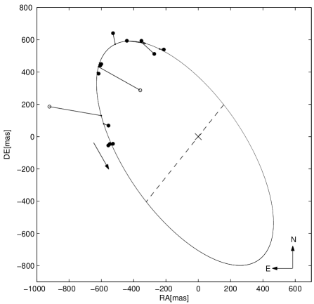
Figure 6: Relative orbit of $\zeta$ Phe on a plane of the sky, for a detailed description see Fig. 3. Two measurements (the open circles) were neglected.

The new times of primary and secondary minimum and their errors were derived using a least-squares fit to the data and by the bisecting-chord method. Only the bottom parts of the eclipses were used. The mean values and the errors for each individual filter are given. Six new times of minimum light were derived using the Hipparcos photometry (Perryman & ESA 1997) and fitting the published light curve. These new times of minima are also included in Table 3. In this Table, the epochs are calculated from the light elements given in Table 1, the other columns being self-explanatory.

$\zeta$ Phe has one of the shortest apsidal motions among the eclipsing binaries (see e.g. Claret & Giménez 1993). Due to a low eccentricity, the amplitude of the effect is small. For an accurate calculation of the apsidal motion rate the method described by Giménez & Garcia-Pelayo (1983) was routinely used. The eccentricity of the orbit in the eclipsing binary is $e^{\prime}=0.0107\pm 0.0020$, the longitude of periastron $\omega_{0}=12.96^{\circ}\pm 5.96^{\circ}$, and the apsidal motion rate $\dot{\omega}=(0.028\pm 0.001)\mathrm{{}^{\circ}/cycle}=(6.16\pm 0.20)\mathrm{{}^{\circ}/yr}$, i.e. the apsidal motion period $U=58.5$ yr. The most recent apsidal-motion analysis is more than 20 years old, made by Giménez et al. (1986), but with no LITE and with a smaller set of times of minima. The eccentricity derived by Giménez et al. was almost the same, but the apsidal motion rate $\dot{\omega}$ was $0.0373~{}\mathrm{{}^{\circ}/cycle}$ and the angle $\omega_{0}~{}=~{}13^{\circ}.$

Our approach was a combination of the two different effects. The behaviour in the $O-C$ diagram was described as a sum of apsidal motion and LITE contribution $(O-C)=(O-C)_{apsid}+(O-C)_{LITE}$, distinguishing the primary and secondary minima. It means the least-squares algorithm was minimizing the $\chi^{2}_{comb}$ with respect to 12 parameters in total ($A,p_{3},i,e,\omega,\Omega,T_{0},JD_{0},P,\dot{\omega},\omega_{0},e^{\prime}$).

Table 3: The new minima timings of $\zeta$ Phe based on photoelectric observations.

HJD-2400000	Error	Prim/Sec	Epoch	Ref.
47872.7742	0.005	Sec	3730.5	[1]
47873.6172	0.005	Prim	3731.0	[1]
48187.535	0.005	Prim	3919.0	[1]
48397.0807	0.005	Sec	4044.5	[1]
48484.7523	0.005	Prim	4097.0	[1]
48508.9557	0.005	Sec	4111.5	[1]
51466.9675	0.0005	Prim	5883.0	[2]
51467.7907	0.001	Sec	5883.5	[2]
53622.6453	0.0001	Prim	7174.0	[3]
53623.4710	0.0001	Sec	7174.5	[3]

• [1] - Perryman & ESA 1997; [2] - Shobbrook (2004); [3] - This paper;

The astrometric solution based on the combined app-roach is satisfactory, while the older measurements have larger scatter than the recent ones (the old ones are visual, while the modern ones are speckle-interferometric). Two measurements were neglected, because of their large scatter (see Fig.6). Our solution led to the parameters listed in Table 1, which could be compared to previously found values. Most recently Ling (2004) reported the parameters: $p_{3}~{}=~{}210.4$ yr, $e~{}=~{}0.348$, $a~{}=~{}804$ mas, $i~{}=~{}61.9^{\circ}$, $\Omega~{}=~{}33.5^{\circ}$, $\omega_{3}~{}=~{}271.7^{\circ}$. It is evident that the new parameters are in very good agreement with these ones. The new values imply the mass function of the distant body $f(M_{3})=0.056~{}\mathrm{M_{\odot}}$. With the masses of the primary and secondary component of the eclipsing binary $M_{1}=3.93~{}$$\mathrm{M_{\odot}}$ and $M_{2}=2.55~{}\mathrm{M_{\odot}}$ (Andersen 1983), one could derive the mass of the astrometric third body $M_{3}=1.73~{}$$\mathrm{M_{\odot}}$. This value corresponds to a spectral type around A7, which is in excellent agreement with the photometric analysis (Clausen et al. 1986).

3.3 HT Vir

One member of the visual binary STF 1781 is the eclipsing binary system HT Vir (ADS 9019, HD 119931, HIP 67186, BD+05 2794, $V~{}=~{}7.2$ mag, sp F8V). HT Vir is a contact W UMa system, with a period of about $0.4$ d and the depths of minima of about $0.4$ mag. Both visual components have almost equal brightness. The third component of the system is brighter than the eclipsing binary HT Vir during its eclipses and fainter than it during its maxima.

According to Walker & Chambliss (1985) the distant astrometric component was discovered by Wilhelm Struve in 1830 at a separation of about 1.4 ^′′  and position angle $240^{\circ}$. Since then, numerous astrometric observations were obtained (altogether 277, from which 275 were used in our analysis) and the orbit is almost completely covered by the observations.

Figure 7: Relative orbit of HT Vir on a plane of the sky, for a detailed description see Fig. 3.

Baize (1972) suggested that the star might be variable. After then, Walker & Chambliss (1985) obtained a complete light curve of HT Vir and did the first analysis. It indicated that both components of the eclipsing pair are almost identical and in contact. The temperatures of both components are about $6000~{}\mathrm{K}$ and the spectral type is estimated as F8V for the primary and a little bit earlier for the secondary, the inclination is close to $90^{\circ}$. The total mass of the eclipsing pair is $M_{12}~{}=~{}2.3~{}$$\mathrm{M_{\odot}}$ (D’Angelo et al. 2006).

Lu et al. (2001) discovered that the distant component is also a binary. They have measured the spectra of the HT Vir eclipsing pair, and discovered also the lines from the third component in the spectra and their RV variations with a period of about $32.45$ d. We therefore deal with a quadruple system.

Despite the spectral analysis and a large set of astrometric observations, there were only a few times of minima published during the last few decades. The main reason is relatively recent discovery of the photometric variability of HT Vir. The first times of minima come from 1979. Since then, there were only 31 observations obtained (see Fig. 8). Four new observations were obtained. The two of them were carried out in Ondřejov observatory with the 65-cm telescope and Apogee AP-7 CCD camera and 1 second exposure time in R filter. This new times of heliocentric secondary minima are $2454175.58494\pm 0.00011$ and $2454195.56170\pm 0.00007$. The next one was observed by L. Brát (Private Observatory), using 8-cm telescope with ST-8 CCD camera, 20 seconds exposure time in R filer, resulting in $2454210.44154\pm 0.00015$, and the last one by R.Dřevěný with ST-7 CCD camera, 60 seconds in R filter, resulting in $2454213.49967\pm 0.00012$. One unpublished observation by M.Zejda was also used and four times of minima by M.Zejda published in Zejda (2004) were recalculated, because the heliocentric correction was wrongly computed.

The final plot of the relative astrometric orbit of HT Vir is in Fig. 7. The results, parameters of the orbit around the common barycentre of the system, are given in Table 1. The values of these parameters ($A,\,p_{3},\,i,\,e,\,\omega,\,\Omega,T_{0},JD_{0},P$) were obtained minimizing the $\chi^{2}_{comb}$.

Walker & Chambliss (1985) published the first rough estimation of the proposed LITE from the astrometric orbit. Their value (0.18 d) is not too far from ours (0.13 d).

The new elements for the astrometric orbit can be compared to those of Heintz (1986), which are the following: $p_{3}~{}=~{}274.0$ yr, $e~{}=~{}0.638$, $a~{}=~{}1010$ mas, $i~{}=~{}42.7^{\circ}$, $\Omega~{}=~{}176.4^{\circ}$, $\omega_{3}~{}=~{}250.0^{\circ}$. As one can see, the period of the new orbit is a bit shorter, but the main differences in these values are the angles $\omega$ and $\Omega$. The same fit to the astrometric data points could be reached with simultaneously transformed values $\omega_{3}\rightarrow\omega_{3}+180^{\circ}$ and $\Omega\rightarrow\Omega+180^{\circ}$. This only means the interchange of the role of the two components. This result indicates the incorrect identification of the variable HT Vir in the system in our analysis (the variable was supposed to be the component A) and also in the WDS catalogue, see WDS notes. While Pribulla & Rucinski (2006) correctly identified the variable HT Vir as the B component and A as a single-lined binary.

If we adopt these parameters to estimate the mass function of the distant pair (mass function of the whole pair, not the individual components), we obtain $f(M_{3})~{}=~{}0.17~{}$$\mathrm{M_{\odot}}$. This is quite a high value, dictated by the large amplitude of the LITE. With the total mass of the primary and secondary $M_{12}=2.3$ $\mathrm{M_{\odot}}$ we get the third mass of $M_{3}=2.10~{}$$\mathrm{M_{\odot}}$. The mass of the distant pair is quite high (D’Angelo et al. (2006) derived the mass for some 50 per cent lower, $M_{3}=1.15~{}$$\mathrm{M_{\odot}}$), but note that also this object is a binary and we do not know the individual masses. From the spectroscopic observations (we remind that it is a SB1 type binary), we are only able to estimate the mass function of the components, or some upper limit for one of them (we do not know the inclination). Our resulting $M_{3}$ is the total mass of the SB1 pair $M_{3,1}+M_{3,2}$; the limit for the invisible-component mass $M_{3,2}~{}\cdot~{}\sin(i)=0.075~{}$$\mathrm{M_{\odot}}$. If we assume the coplanar orbit, high difference in masses would arise, one component should be much more luminous and also more luminous than the eclipsing pair itself, which is not the case. In fact the whole system is not coplanar (see e.g. $i=315.5^{\circ}$ and the inclination of the EB close to $90^{\circ}$). If we assume two approximately equal masses, there is a problem with the luminosity, because the distant pair has to be roughly as luminous as the eclipsing pair. This could only be satisfied if one component is underluminous or degenerate.

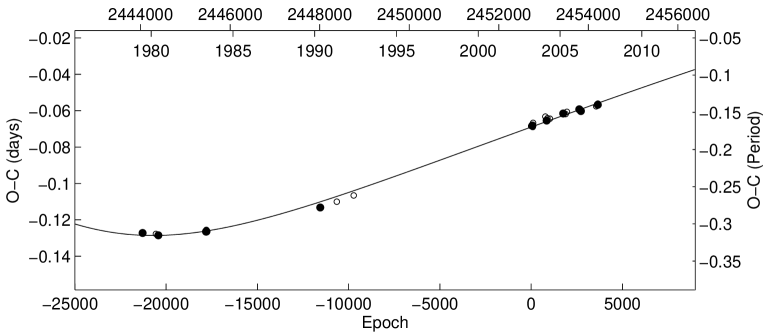
Figure 8: An $O-C$ diagram of HT Vir. The description is the same as in the previous $O-C$ figures, all minimum times are photoelectric or CCD ones.

We have to take into consideration also the comment on the light-curve solution by Walker & Chambliss (1985). Using the Wood’s model, they discovered that if the third light $L_{\mathrm{3}}$ is fixed to be equal to the light from the distant visual component (it means $L_{\mathrm{3}}=0.5$), the solution of the light curve is unrealistic. To conclude, the system could be much more complicated than the approach we have used here. Especially because of the resultant mass and luminosity of the distant pair, the body causing the astrometric variation is probably different from the one causing LITE, but this conclusion will be proven only if also the nonlinear part of the $O-C$ diagram is covered.

4 Discussions and conclusion

Although the number of systems where the astrometric orbit of the third component has been measured together with the presence of LITE is growing steadily, in the most cases only very limited coverage, both in astrometry and times of minima is available. Especially due to this reason the combined analysis of these systems is still difficult, the results are not very convincing and the resultant parameters are affected by relatively large errors.

During the last decade a few papers combining the approach of simultaneous solution of radial velocities, spectral analysis, astrometry, Hipparcos measurements or LITE were published. Besides the systems mentioned in the introduction (V505 Sgr, QS Aql, 44 Boo, QZ Car, SZ Cam, GT Mus, and V2388 Oph) there were also the analyses of V1061 Cyg (combining the light curve analysis, radial velocity analysis, light-time effect and Hipparcos measurements, see Torres et al. 2006), the papers where the radial velocity measurements and astrometry were combined (see Muterspaugh et al. (2006) for the solution of LITE system V819 Her, or Gudehus (2001) for $\mu$ Cas), the paper on HIP 50796 combining the radial velocities with the Hipparcos abscissa data (Torres 2006), or the paper on $\delta$ Lib comparing the results from the period analysis, light-curve analysis, spectral analysis, radio emission and astrometry, respectively; see Budding et al. (2005).

Three eclipsing binaries were studied in this paper. In the case of VW Cep, where the orbits in both methods have relatively best coverage, the distant body satisfies the limits for the luminosities, and also the systemic velocity variations coincide with our hypothesis. New results are comparable with the previous ones. An additional fourth body was introduced to describe the long-term variation in times of minima. The system is probably more complicated than we assumed (chromospheric activity cycles, stellar spots and flares), and we decided to explain only the most pronounced effects in the $O-C$ diagram. Using this combined approach it is possible to derive the parallax of VW Cep more precisely than in previous papers, resulting in $\pi=(35.85~{}\pm$ $\pm~{}0.37)~{}\mathrm{mas}$. The system $\zeta$ Phe displays an apsidal motion together with LITE and this explanation fits the $O-C$ residuals quite well. The quality of the astrometry is worse, but the main result about the masses and the spectral type of the third body is in an excellent agreement with the previous photometric analysis. The last system HT Vir is the case where the new resultant parameters of the distant body are about 2 times larger than one would expect. This could be due to the fact that only a few times of minima were observed in the linear part of the $O-C$ diagram, new minima are needed in the next decades.

The final result is that the method itself is potentially very powerful but it is also very sensitive to the quality of the input data, especially if the method is used for determining the distances of these binaries. It can only be applied successfully in those cases where the astrometric orbit and the LITE in the $O-C$ diagram are well defined by existing observations.

References

- [1] Albayrak, B., Fikri Özeren, F., Ekmekçi, F., Demircan, O.: 1999, RMxAA 35, 3
- [2] Andersen, J.: 1983, A&A 118, 255
- [3] Baize, P.: 1972, A&AS 6, 147
- [4] Binnendijk, L.: 1966, PDAO 13, 27
- [5] Borkovits, T., Hegedues, T.: 1996, A&AS 120, 63
- [6] Budding, E., Bakis, V., Erdem, A., Demircan, O., Iliev, L., Iliev, I., Slee, O.B.: 2005, Ap&SS 296, 371
- [7] Claret, A., Giménez, A.: 1993, A&A 277, 487
- [8] Clausen J.V., Gyldenkerne, K., Gronbech, B.: 1976, A&A 46, 205
- [9] Dachs, J.: 1971, A&A 12, 286
- [10] D’Angelo, C., van Kerkwijk, M.H., Rucinski, S.M.: 2006, AJ 132, 650
- [11] Docobo, J.A., Ling, J.F.: 2005, IAU Commission on Double Stars, 1
- [12] Frieboes-Conde, H., Herczeg, T.: 1973, A&AS 12, 1
- [13] Giménez, A., Clausen, J.V., Jensen, K.S.: 1986, A&A 159, 157
- [14] Gimenez, A., Garcia-Pelayo, J.M.: 1983, Ap&SS 92, 203
- [15] Groeneveld, I.: 1947, VeHei 14, 43
- [16] Gudehus, D. H.: 2001, Bulletin of the American Astronomical Society, 33, 850
- [17] Guthnick, P.: 1931, \an 241, 263
- [18] Guthnick, P., Prager, R.: 1934, \an 251, 257
- [19] Harmanec, P.: 1988, BAICz 39, 329
- [20] Harmanec, P., Horn, J.: 1998, JAD 4, 5
- [21] Heintz, W.D.: 1986, A&AS 64, 1
- [22] Heintze, J.R.W., Spronk, W., Hoekzema, N.: 1989, SSRv 50, 344
- [23] Hendry, P.D., Mochnacki, S.W.: 2000, ApJ 531, 467
- [24] Herczeg, T., Schmidt, H.: 1960, VeBon 57, 1
- [25] Hill, G.: 1989, A&A 218, 141
- [26] Hogg, A.R.: 1951, MNRAS 111, 315
- [27] Holmgren, D.: 1987, BAVSO, 709
- [28] İbanoǧlu, C., Çakirli, Ö., Deǧirmenci, Ö., Saygan, S., Ulaş, B., Erkan, N.: 2000, A&A 354, 188
- [29] Irwin, J.B.: 1959, AJ 64, 149
- [30] Kallrath, J., Linnell, A.P.: 1987, ApJ 313, 346
- [31] Kaszas, G., Vinko, J., Szatmary, K., Hegedus, T., Gal, J., Kiss, L.L., Borkovits, T.: 1998, A&A 331, 231
- [32] Knipe, G.F.G.: 1971, PASP 83, 352
- [33] Knipe, G.F.G.: 1972, MNSSA 31, 27
- [34] Kvíz, Z., Zejda, M., Kohoutek, L., Grygar, J.: 1999, IBVS 4739, 1
- [35] Kwee, K.K.: 1966, Bull. Astron. Inst. Netherlands 18, 448
- [36] Kwee, K.K., van Woerden, H.: 1956, Bull. Astron. Inst. Netherlands 12, 327
- [37] Lázaro, C., Arévalo, M. J., Antonopoulou, E.: 2006, MNRAS 368, 959
- [38] Ling, J.F.: 2004, ApJS 153, 545
- [39] Lorenz, R., Mayer, P., Drechsel, H.: 1998, A&A 332, 909
- [40] Lu, W., Rucinski, S.M., Ogłoza, W.: 2001, AJ 122, 402
- [41] Mallama, A.D.: 1981, PASP 93, 774
- [42] Mason, B.D., Wycoff, G.L., Hartkopf, W.I., Douglass, G.G., Worley, C.E.: 2001, AJ 122, 3466
- [43] Mayer, P.: 1990, BAICz 41, 231
- [44] Mayer, P.: 1997, A&A 324, 988
- [45] Mayer, P.: 2004, ASP Conf. Ser. 318, 233
- [46] Menzies, J.W., Cousins, A.W.J., Banfield, R.M., Laing, J.D.: 1989, SAAOC 13, 1
- [47] Muterspaugh, M.W., Lane, B.F., Konacki, M., Burke, B.F., Colavita, M.M., Kulkarni, S.R., Shao, M.: 2006, A&A 446, 723
- [48] Perryman, M.A.C., ESA: 1997, The Hipparcos and Tycho catalogues
- [49] Popper, D.M.: 1948, ApJ 108, 490
- [50] Pribulla, T., Chochol, D., Tremko, J., Parimucha, S., Vanko, M., Kreiner, J.M.: 2000, CoSka 30, 117
- [51] Pribulla, T., Rucinski, S.M.: 2006, AJ 131, 2986
- [52] Ribas, I., Arenou, F., Guinan, E.F.: 2002, AJ 123, 2033
- [53] Rovithis-Livaniou, H., Rovithis, P., Antonopoulou, E., Kalimeris, A.: 1991, IBVS 3608, 1
- [54] Schilt, J.: 1926, ApJ 64, 215
- [55] Shobbrook, R.R.: 2004, JAD 10, 1
- [56] Skillman, D.R.: 1982, JAAVSO 11, 57
- [57] Torres, G.: 2004, ASP Conf. Ser. 318, 123
- [58] Torres, G.: 2006, AJ 131, 1022
- [59] Torres, G., Lacy, C.H., Marschall, L.A., Sheets, H.A., Mader, J.A.: 2006, ApJ 640, 1018
- [60] van der Wal, P.B., Nagel, C., Voordes, H.R., Boer, K.S.: 1972, A&AS 6, 131
- [61] Walker, R.L., Chambliss, C.R.: 1985, AJ 90, 346
- [62] Yakut, K., Kalomeni, B., İbanoğlu, C.: 2004, A&A 417, 725
- [63] Zejda, M. 2004, Informational Bulletin on Variable Stars, 5583, 1