The network approach:
basic concepts and algorithms

1 The network approach as a physical problem

As economists are the experts on consumer attitudes and sociologists on human social interaction, physicists are the experts simplifying complex problems. However, one usually does not ask a physicist about stock-market forecasts stockmarket , neither does one immediately think of a physicist when the issue concerns controlling civilian crowds helbing . Scientists dealing with many complex real problems do not take kindly to the propensity of physicists entering their field of study and proposing overly simplified theories. One even often hears jokes about physicists assuming chickens to be spherical. Though, such kind of simplifications and assumptions do turn out to be rather helpful in solving a specific real-life problem at times.

Of course, not all assumptions can be taken. They must retain the essential features to explain what we observe. Take a balloon filled with air, for instance. The complicated system we call ‘air’ comprehends a huge number of molecules of nitrogen, oxygen, argon and carbon dioxide, among many other. Each one of these molecules is an arrangement of atoms with different weights, and even each atom is a system of quarks and electrons interacting according to specific forces. To explain why a balloon expands while being filled with air, you do not need to think about all these details. One just assumes that air is a set of small spheres traveling in all directions and colliding among them and with the walls of the balloon. These collisions are essentially what is responsible for what we call gas pressure. Everything else can be ignored.

This way of dealing with reality, trying to simplify it down to its elementary components and interactions for explaining a certain phenomenon is what leads physicists to uncover fundamental laws of nature. And schematically, it is also precisely what the so-called network approach is about: the components of the system under study are reduced to elements that retain the essential features we want to address and the interactions between such components are represented by links joining the elements livro2 . Elements could be molecules with links representing the collisions among them, but they could also be seen as persons linked by their friendship acquaintances or as enterprises connected among them according to the trades they establish.

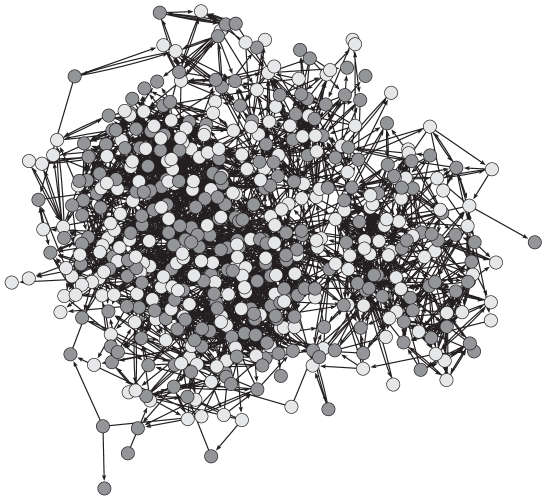
Figure 1: Illustration of a network of different social friendships in a U.S. School addhealth . Different gray tonalities distinguish between male and female students. Arrows indicate who points who as a friend.

The use of the network approach to solve problems goes back to the eighteenth century, when Leonhard Euler wanted to solve the “Seven Bridges of Königsberg” problem. The city of Königsberg – now called Kaliningrad, located in Russia – is set on both sides of Pregel River, having two islands in between. Both islands are connected with each other and with both sides of the river by seven bridges, and Euler posted the problem of proving whether it is possible to cross each bridge exactly once and return to the starting point. By solving it, showing that such a walk does not exist, Euler introduced the concept of graph as the mathematical object composed by nodes (the elements) and edges (the connections) and founded the so-called graph theorylivro . Recently, physicists adopted instead the term network and, with the help of computers, developed the network approach to solve a range of new problems spanning physics, biology, sociology, and economics. Since the underlying networks have a very complicated structure as the one sketched in Fig. 1, it is common to refer them as complex networks. Several reviews and books on complex network research have been published livro2 ; albert02 ; dorogovtsevrev ; newman03 ; boccaletti06 ; dorogovtsev07 in the last decade.

A good way to understand why such an approach is indeed helpful is to present some of its main achievements. In this Chapter we will briefly describe the main theoretical and numerical tools as well as computational algorithms developed to construct and study networks. In Sec. 2 the main types of networks are described and in Sec. 3 the fundamental properties to characterize a network are given. In Sec. 4 three families of networks are described, namely random networks, small-world networks and scale-free networks and a brief overview over the recent trends in network approach are given in Sec. 5.

2 Classification of networks

A network consists of nodes and edges. The features we address to the nodes and to the edges depend on what we want to study. Therefore, the first thing to do when constructing a network is to know what kind of components and interactions between them are we talking about. Figure 2 summarizes the main kinds of nodes and connections in networks.

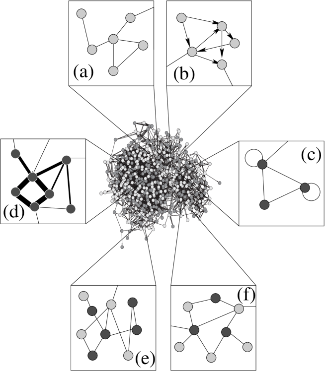
Figure 2: Classification of networks. Illustration of parts of a network that are (a) undirected, (b) directed, (c) with self-connections, (d) weighted, (e) monopartite, where the nature of the node does not influence the existence of connection and (f) bipartite, where nodes of one kind only connect to nodes of the other kind.

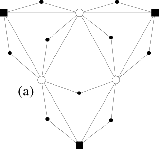
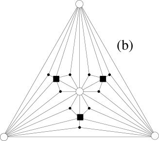
Figure 3: Two examples of deterministic networks: (a) the pseudo-fractal network dorogovtsevrev and (b) the Apollonian network hans05 . Different symbols for the nodes represent different generations during the construction procedure (see text).

We start by discussing the interactions. As in physics, social and economical systems involve interactions that may or may not be symmetric. For instance, a friendship connection between two persons, $i$ and $j$, is symmetric, in the sense that there is no preferred direction connecting $i$ to $j$ or vice-versa. Therefore, edges as the ones illustrated in Fig. 2a are sufficient to represent the connections between people that are friend of each other. Conversely, if we want to see which people a given person knows inside a social system, then there will be for sure some people more famous than other, independent of their number of friends. Person $i$ knowing person $j$ does not guarantee that person $j$ also knows person $i$. A direction must be given and therefore one uses arrows to represent interactions, as shown in Fig. 2b.

Networks composed by symmetric interactions (edges) are called undirected networks, while networks composed by arrows are called directed networks. While this difference between symmetric and asymmetric interactions may seem subtle or spurious it has enormous implications in the way dynamical processes take place on the corresponding networks. For instance, in rumor propagation or flux of money or information boccaletti06 ; dorogovtsev07 .

The two counter parts of symmetric and asymmetric interactions appear only in connections joining different nodes. But it may be the case that self-connections, as the ones illustrated in Fig. 2c, play an important role in a network. Recently it was shown hellstein07 that in a network of authors where connections represent citations to other authors, self-citations are an important feature to track the shifting of scientists from one field to another.

Further, after establishing the nature of the interactions, there is still the possibility to address a value (or weight) to the connection. For instance, the number of phone calls between two persons in a social system may be regarded as a measure of the friendship closeness of those two individuals martaNature . Figure 2d illustrates weighted connections, opposite to Fig. 2a where connections are unweighted.

As for the nature of the nodes they may determine if connections may exist between them or not. If nodes are people and connections join the people that are co-authors of the same paper, then no restriction from the nodes itself is imposed. Some of the persons may be men and other women. It will make no difference for the connections, as illustrated in Fig. 2e. But it may be the case that the nature of the nodes strongly biases the occurrence of a connection of some sort between them. For instance, in a network where nodes are either men and women and connections represent intimate relations between them, during their life times, one expects a stronger tendency for men being attached to women and vice-versa, as illustrated in Fig. 2f. This particular kind of structure where nodes of one sort are connected to nodes of the other sort is known as a bipartite structure, opposite of monopartite structures. In general, multipartite networks are also sometimes addressed, for instance in an ecological system where connections represent trophic relations between several different species.

Of course, these features described above may appear solely or combined. For instance, a network where the interactions measure the number of phone calls done by a given person $i$ to another person $j$ has connections that are directed ($i$ calls $j$) and weighted (number of phone calls).

Altogether, these network ingredients compose the bulk of the fundamental ways for constructing a network underlying a real system. However, as mentioned earlier they have a very complicated structure, which in general, is very difficult to be studied analytically. The main reason lies in the fact that the distribution of nodes and connections is associated with some stochastic or probabilistic events. Therefore, analytical study of networks is usually done in some prototypical deterministic networks that contain the structural properties of the real networks we want to study.

Deterministic networks are constructed iteratively by introducing new nodes with a certain deterministic rule. In Fig. 3 we show two examples of deterministic networks. The first one is the so-called pseudo-fractal network dorogovtsev02 : one starts from three interconnected nodes, and at each iteration each edge generates a new node, attached to its two vertices. At a certain iteration $n$, the number of nodes is given by $N_{n}=\tfrac{3}{2}(3^{n}+1)$ and the number of connections by $V_{n}=3^{n+1}$. The second one is the Apollonian network which is constructed in a different way: one starts with three interconnected nodes, defining a triangle; at $n=0$ one puts a new node at the center of the triangle and joins it to the three other nodes, thus defining three new smaller triangles; at iteration $n=1$ one adds at the center of each of these three triangles a new node, connected to the three vertices of the triangle, defining nine new triangles and so on. In this case one has $N_{n}=\tfrac{1}{2}(3^{n+1}+5)$ and $V_{n}=\tfrac{3}{2}(3^{n+1}+1)$.

In Section 4 we will see that some of the characteristics of these two networks are ubiquitous in real systems. Next, we will introduce the main tools that enable to uncover the structure of complex networks.

3 Characterization of networks

After knowing the main ingredients to construct a network the next task is to know what measurements are needed to understand the structure. In this Section we will briefly address the main statistical and topological properties in network research. For more details the reader may be interested in a recent review boccaletti06 .

The core of all the panoply of properties described below is the so-called adjacency matrix ${\cal A}$. It is defined by elements $a_{ij}$ that are different from zero only if there is one connection linking $i$ to $j$. If the network is undirected, ${\cal A}$ is symmetric ($a_{ij}=a_{ji}$). Further, if the network is unweighted then the elements are either $0$ (not connected) or $1$ (connected), while for weighted networks $a_{ij}$ takes real values within a given range.

Since networks can be considerably large and adjacency matrices are typically sparse, when implementing it in a computer program one usually uses the mapping of the adjacency matrix into a $2$-linked lisk, which is a $M\times 2$ matrix, mat_adj(m,n), with m$=1,\dots,M$ labelling the connections and n$=1,2$ indicating the two vertices of one connection. The connection m from $i$ to $j$ is then defined by the two entries mat_adj(m,1)$=i$ and mat_adj(m,2)$=j$. Notice that for undirected networks one needs in fact a $2M\times 2$ matrix, since each connection must be defined from $i$ to $j$ and simultaneously from $j$ to $i$.

In the following we will focus on the simplest case of undirected and unweighted networks. Extensions to all other types of networks are straightforward.

3.1 Degree distribution and correlations

Within a network, each node $i$ has a certain number of connections which can be measured by its degree

$$k_{i}=\sum_{j}a_{ij}.$$ (1)

The degree of a node takes integer values for unweighted networks and real values for weighted networks. For directed networks the degree in Eq. (1) equals the so-called outgoing degree, $k_{i}^{(out)}$. The number of incoming connections is then measured by $k_{i}^{(in)}=\sum_{j}a_{ji}$.

With the degree of each node one easily computes the degree distribution $P(k)$, which equals the fraction of nodes having degree $k$. As we will see this topological quantity is able to distinguish between different network families. In some cases, it may yield large fluctuations, especially when networks are not large enough as frequently happens in empirical systems. For that, one may prefer to compute the cumulative distribution $P_{cum}(k)=\sum_{k^{\prime}>k}P(k^{\prime})$.

The degree distribution, however, does not tell about the correlations between the nodes. For instance, what is the probability that a node with degree $k$ is connected to a node with degree $k^{\prime}$? The answer of course, is the conditional probability $P(k^{\prime}|k)$, that also defines the average degree of the nearest neighbors of nodes with degree $k$

$$k_{nn}(k)=\sum_{k^{\prime}}k^{\prime}P(k^{\prime}|k).$$ (2)

If there are no correlations, then the conditional probability is independent of $k$ and $k_{nn}(k)=\langle k^{2}\rangle/\langle k\rangle$. If the network is correlated, then $k_{nn}(k)$ varies with $k$ and the two cases may be distinguished. When $k_{nn}(k)$ increases with $k$, i.e. nodes with similar degrees tend to be connected, the network is called assortative. This is the most typical situation found in social networks. Oppositely, if the less connected nodes are preferentially attached to the most connected ones, $k_{nn}(k)$ decreases with $k$ and the network is called disassortative. Biological networks are examples of disassortative networks.

3.2 Clustering coefficient and cycles

From the degree distribution and degree-degree correlations we are able to know how many neighbors we should expect to observe when picking randomly a node in the network and what is the expected degree of its neighbors. The next question is: which nodes are neighbors of the neighbors of a given node? Are they also neighbors of the given node?

To answer these questions, other quantities are introduced. To know which neighbors are neighbors between them, one just measures the fraction of connection among the neighbors of a given node from all possible connections, yielding the so-called clustering coefficient watts98 . A node $i$ with $k_{i}$ neighbors yields $k_{i}(k_{i}-1)/2$ possible connections between them in the case of an undirected network, $k_{i}(k_{i}-1)$ for a directed one, and therefore, if there are only $m_{i}$ connections between the neighbors the (undirected) clustering coefficient is just

$$C_{3}=\frac{2m_{i}}{k_{i}(k_{i}-1)}=\frac{\sum_{j,n}a_{ij}a_{jn}a_{ni}}{k_{i}(k_{i}-1)},$$ (3)

where the last member shows explicitly how to count the number of existing edges between neighbors of node $i$.

The quantity $m_{i}$ in Eq. (3) counts the number of cycles with size three (triangles) containing node $i$. That’s the reason why we label the clustering coefficient with the subscript $3$. Triangles are the smallest cycles within a network. But one could think of cycles with larger size to know about non-local features of the network. In bipartite networks for instance such larger cycles are important, since they have no triangles and therefore the clustering coefficient in Eq. (3) cannot provide any useful informationlind05 .

In general, the number of cycles of size $n$ containing a specific node $i$ are given by

$$N_{c}(i,n)=\sum_{j_{1}\dots j_{n-1}}a_{ij_{1}}a_{j_{1}j_{2}}\dots a_{j_{n-1}i}.$$ (4)

In practice it is very expensive to count $N_{c}$ for arbitrary $n$. Two different approaches are used instead. One is to use Monte Carlo algorithmsrozenfeld05 , based on large samples of random walks trough the connections and counting how many times one returns to the starting node. The other is to estimate the number of larger cycles by counting only small cycles, typically triangles and squareslind05 ; vazquez05 .

3.3 Average shortest path length

The cycles mentioned previously are closed paths whose statistical features provide information about the underlying network beyond the node’s local vicinity. Related with cycles is the question of how far are two given nodes in a network, which leads naturally to the concept of average shortest path length.

The average shortest path length $\ell$ is the average number of connections joining two randomly chosen nodes. Of course, $\ell$ increases with the network size $N$ and an important point is to ascertain how fast is this increase. If $\ell$ increases slowly, typically with $\ln{N}$, then two given nodes are typically near each other, illustrating what is called the small-world effect watts98 .

Though simple to understand, the average shortest path length is not trivial to compute efficiently, since it concerns the determination of the shortest path from all existing paths between two nodes. An efficient algorithm to compute $\ell$ is the Dijkstra algorithm which is a sort of a burning algorithm of the breadth-first search type. One starts from a given node and visits only one single time each one of the other nodes in the network, first the nearest neighbors ($\ell=1$), then the next-nearest neighbors ($\ell=2$) and so on. An implementation in Fortran of the Dijkstra algorithm is as follows:

     avpl = 0.0d0
     do 1000 node=1,Nnodes   !Loop in the nodes
        avplnode    = 0.0d0
        flg         = 0
        pathlength  = 0
        path        = 0
        nactualsite = 1
        site(1)     = node
        do i=1,Nnodes
           vs(i) = 1
        enddo
        vs(site(1)) = 0
        do while (flg.eq.0)
           pathlength = pathlength + 1
           nsite      = 0
           do actualsite=1,nactualsite !Loop on node layer
              do 1100 i=1,Nedges    !Loop in the connections
                 if(mat_adj(i,1).ne.site(actualsite))goto 1100
                 if(vs(mat_adj(i,2)).eq.0)goto 1100
                 path             = path  + 1
                 avplnode         = avplnode+float(pathlength)
                 nsite            = nsite + 1
                 nextsite(nsite)  = mat_adj(i,2)
                 vs(mat_adj(i,2)) = 0
1100          continue
           enddo
           if(nsite.eq.0)then   !All nodes where visited
              flg=1
           else                 !... if not ...
              nactualsite = nsite
              do i=1,nsite
                 site(i)=nextsite(i)
              enddo
           endif
        enddo
        avpl=avpl+avplnode/float(path)
1000 continue     !END loop in the nodes
     avpl = avpl/float(Nnodes)

Such routine is intended for empirical networks, where the adjacency matrix is taken as input. For artificial networks, the algorithm could be implemented more efficiently by constructing a distance matrix, while saving the entries for the adjacency matrix during the construction procedure.

3.4 Community decomposition

The clustering coefficient mentioned above can be formulated in a more general form. How large can a strongly connected vicinity of a given node be? This question leads to the concept of community: some subset of nodes in the network whose density of connections between them is larger than the density of connections to or from the exterior of that subset.

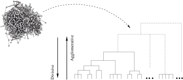
Figure 4: Sketch of the mapping of a network (left) into a dendrogram (right). The dendrogram can be constructed using either agglomerative or divisive algorithms (see text).

Having a network with $N$ nodes and $M$ connections one can define the average density of connections as $\rho_{Net}=2M/(N(N-1))$. Similarly, any subset of this network with $n$ nodes and $m_{in}$ connections between them would have an average density $\rho_{in}=2m_{in}/(n(n-1))$. If, besides the $m_{in}$ connections between the nodes composing the subset, there are other $m_{out}$ connections between the $n$ nodes and the remaining $N-n$ nodes outside the subset, the corresponding density is $\rho_{out}=m_{out}/(n(N-n))$. For the subset to be a community the following condition must be satisfiedreichardt04

$$\rho_{out}<\rho_{Net}<\rho_{in}.$$ (5)

This condition, however, does not define a community in a unique way. Different community structures, in size and number, can simultaneously satisfy condition (5) for the same network. Thus, different methods to detect communities have been proposed livroSoc ; girvan02 ; newman04 ; palla05 .

The traditional method is the so-called hierarchical clusteringlivroSoc that maps the network into a dendrogram, as illustrated in Fig. 4. One starts with all nodes of the network and no edges (bottom of the dendrogram), addressing to each pair of nodes, $i$ and $j$, a weight $w_{ij}$ that measures how close connected are the nodes. This weight could be given by the inverse of the shortest path length joining the two nodes, $w_{ij}=1/\ell_{ij}$. Then iteratively, one adds the links between pairs of nodes following the decreasing order of the weights, which leads to the agglomeration of small groups of nodes into larger and larger communities. This method is thus agglomerative.

The dendrogram can also be constructed in the reverse direction (top-down): one starts with the entire network of nodes and edges and iteratively cuts the edges, thus dividing the network into smaller and smaller groups girvan02 . This method is called divisive and the central point is which edges should be cut at each iteration. A good criterion is based on the computation of the so-called betweenness of each edge, that counts the number of shortest path lengths crossing that edge. Having the betweenness of each node one follows the decreasing order of betweenness while cutting the edgesgirvan02 ; newman04 .

Both agglomerative and divisive algorithms for community detection assume that communities do not intersect with each other. However, in real systems this is not the common situation. To overcome this drawback a different algorithm was proposedpalla05 , that enables the detection of communities that overlap each other. In the heart of this algorithm is the concept of $k$-clique, a complete subgraph of size $k$, i.e. a subgraph with $k$ nodes where each node is connected to the remaining $k-1$ nodes. Detecting all $k$-cliques in the network, a $k$-clique community is then defined as the union of all $k$-cliques that can be reached from each other.

The investigation of how to detect communities is one of the most recent topics in network research and has attracted huge attention, since communities are ubiquitous in real networking systems and are crucial for the understanding of their structure and evolution,

4 Three important network topologies

	Random	Small-world	Scale-free
$P(k)$	$\hbox{e}^{-\bar{k}}\bar{k}^{k}/k!$	$\hbox{e}^{-\bar{k}}\bar{k}^{k}/k!$	$2m^{2}/k^{3}$
$C_{3}$	$\bar{k}/N$	$C_{0}(1-p)^{3}$	$\sim N^{-3/4}$
$\mathbf{\ell}$	$\ln{N}/\ln{(pN)}$	$\ln{N}$	$\ln{N}/\ln\ln{N}$

Table 1: Distinguishing different complex topologies with the degree distribution $P(k)$, clustering coefficient $C_{3}$ and average shortest path length $\ell$. Here $N$ is the total number of nodes, $p$ is the probability for two nodes to be connected, $\bar{k}$ is the average number of connections per node, $C_{0}$ is the clustering coefficient of the regular network from which the small-world network is constructed, and $m$ is the number of initial connections of each new node in a scale-free network (see text).

With the main statistical and topological tools described above it will be now possible to briefly present the main families of networks that are usually studied. In this Section we will describe the fundamental properties of Random, Small-world and Scale-free networks, and explain how to construct them. Table 1 summarizes their fundamental properties. For the interested reader, the reviews cited above livro2 ; albert02 ; dorogovtsevrev ; newman03 ; boccaletti06 ; dorogovtsev07 provide additional information.

4.1 Random networks

Random networks were introduced by Erdös and Rényi in the late fiftieserdos to study organizing principles underlying some real networks. To construct them, one defines the probability $p\equiv p(N)$, function of the total number $N$ of nodes, which determines the probability for a pair of nodes to be connected, and applies it to the $N(N-1)/2$ pairs of nodes. The connections are typically long-range connections, and no degree-degree correlations are found.

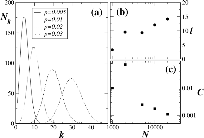
Figure 5: Characterization of Random Networks. (a) The degree distribution $P(k)=N_{k}/N$ for different values of the connection probability $p$, with $N=2000$ nodes and (b) the average shortest path length $\ell$ and (c) the clustering coefficient $C$, as a function of the network size $N$ fixing $p=0.01$.

The degree distribution is typically Poissonian, as shown in Fig. 5a and an important feature of random networks, which also appears in real networks, is their small average shortest path length $\ell$. As illustrated in Fig. 5b, typically $\ell$ increases not faster than logarithmically with the network size. Another typical feature of Random Networks is their small clustering coefficient which typically decreases with the network size as $1/N$ for sufficiently large $N$, as sketched in Fig. 5c.

One main goal in studying random networks is to determine the critical probability $p_{c}(N)$, beyond which some specific property is more likely to be observed, e.g. the critical probability marking a transition to percolation christensen98 .

4.2 Small-world networks

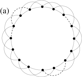
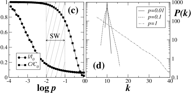
Figure 6: To construct a Small-world Network we start with a (a) regular network and choose a fraction $p$ of connections to be (b) rewired randomly to other nodes. For a certain range of $p$-values one finds (c) The Small-world (SW) regime, characterized by large clustering coefficients $C$ and small average shortest path length $\ell$, when compared to the values $C_{0}$ and $\ell_{0}$ found for the regular network in (a). (d) The degree distribution of Small-world networks is typically peaked for small $p$ and converges to a Poissonian for large $p$.

While reproducing fairly the shortest path length of many empirical networks, random networks have also a small clustering coefficient, which is not typical, e.g., social networks. In fact, many social networks have simultaneously small $\ell$ and large $C$, i.e. two persons are typically close to each other in the friendship connection web and his/her friends tend to be also friends of each other.

To reproduce such a topology Watts and Strogatz proposed watts98 a simple algorithm to construct networks yielding both features. Starting with $N$ nodes disposed in a chain and connected with its $k_{0}$ nearest neighbors (Fig. 6a) one rewires each connection with probability $p$. As illustrated in Fig. 6b, such procedure yields a network composed mainly by short-range connections with a few number of long-range connections.

While the small number of long-range connections are sufficient to guarantee a small average shortest path length, the short-range connections keep the clustering coefficient significantly high, if one compares with the random network counterpart. Figure 6c shows both $C$ and $\ell$ as function of the rewiring probability $p$. For large $p$ the Watts-Strogatz procedure yields small $C$ and $\ell$ as in random networks, while for small $p$ one has large $C$ and $\ell$ as observed in regular networks. In the middle, typically for $0.01\lesssim p\lesssim 0.1$ we find the Small-world (SW) regime described above.

While sweeping through the spectrum of $p$ values, the degree distribution varies from a $\delta$-function (regular network) to an exponential distribution ($p=1$). In the SW regime the degree distribution is approximately Poissonian, as illustrated in Fig. 6d.

Instead of rewiring short-range connections into long-range ones, an alternate procedure newman99 would be to add new long-range connections for each existing connection in the network, with a probability $p$. This procedure is more appropriate for most purposes, since it avoids the possibility of generating disconnected sets of nodes.

4.3 Scale-free networks

Both random and small-world topologies have other drawbacks. First, they do not evolve, the total number of nodes being fixed from the beginning. Second, there are no criteria from choosing specific pairs of nodes to be linked.

In some real networks, that are growing in time, the new nodes tend to prefer connections with the most connected nodes - so-called hubs - of the existing network. This happens for instance in the World Wide Web. New Internet pages tend to link to the most connected ones.

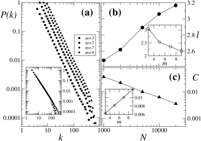
Figure 7: Characterizing evolving Scale-free networks. (a) Power-law degree cumulative distribution $P(k)$ for different values of the initial number $m$ of connections with $N=10^{4}$ nodes and in the inset for different network sizes $N=10^{3},5\times 10^{3},10^{4}$ and $2\times 10^{4}$ with $m=3$. For the same cases one also plots (b) the average shortest path length and (c) the clustering coefficient.

These two additional ingredients, growth and preferential attachment, were addressed by Barabási and Albert barabasi99 to construct networks with similar features as the ones of the WWW. The most crucial feature of these networks is the non-existence of a characteristic number of neighbours: the degree distribution is a power-law $P(k)\sim k^{-\gamma}$. Therefore, it is usual to call such networks, Scale-free networks.

To construct a scale-free network, one starts with a small amount of nodes totally interconnected, and adds iteratively one node with $m$ connections to the previous nodes, chosen from a probability function proportional to their number of connections. With this construction one obtains a degree distribution $P(k)\propto k^{-\gamma}$, where $\gamma\to 3$ as $N\to\infty$, independent of the initial number of fully interconnected nodes and $m$, as illustrated in Fig. 7a.

From Figs. 7b and 7c one also sees that scale-free networks have typically small $\ell$ and $C$, similar to random networks (see also Tab. 1). Further, an increase of the initial number $m$ of connections tends to decrease $\ell$ and increase $C$, as shown in the insets of Figs. 7b and 7c respectively.

From the computational point of view the preferential attachment should be implemented by looking at the existing edges instead of imposing a probability for choosing a node proportional to its degree. In fact, a random choice on the set of existing edges is equivalent to a choice on the set of existing nodes proportional to its degree, and it is much more efficient.

Finally, it is also possible to generate scale-free networks, by either imposing a priori a power-law distribution of all connections randomly distributed, or by following a deterministic iterative rule for new nodes. The first procedure generates what is usually called a generalized random graph albert02 , while the latter concerns among other the deterministic scale-free networks sketched in Fig. 3.

4.4 The landscape analog of complex networks

Some of the topological and statistical quantities described in Sec. 3 were not considered in this Section, namely the degree-degree correlations and the community structure. The main reason being that such quantities may appear differently in any of the above network topologies. To end this Section, we present a pictorial overview recently proposed axelsen06 , to improve the perception of all topologies discussed in this chapter.

Lets imagine that the nodes of a certain network are placed over a landscape. The altitude where each node lies is proportional to its degree, and neighbours are placed closer than other nodes. How would the landscape look like for each different topology?

A regular network as the one picked in Fig. 6a, where all nodes have the same degree, would yield a perfect plateau. Other networks with some typical degree, like random or small-world networks, would have a smooth landscape with some hills alternating with valleys. High mountains would appear, of course, in scale-free networks.

The number of hills or mountains would then depend on the degree-degree correlations. For positively correlated (assortative) networks, where nodes of similar degree tend to connect with each other, a single bump is observed. A classical example of such a network is the Internet. If, on the contrary, high connected nodes have low connected nodes as neighbours (negative correlations), several hills or mountains appear. Examples of such rough landscape can be found in biological systems.

Besides, this nice analog not only catches the main features of the different topologies described above, but also provides new insight for uncovering the hierarchical structure of the complex network axelsen06 .

5 Recent trends in network research

The above Sections hopefully provide a glimpse of what network approach is about. What to do next? What are the main research activities in the field of network research? In a broad sense, three fundamental open questions remain in network research. First, how to model empirical networks from fundamental principles? Second, what new topological or statistical tools could be introduced to improve the uncovering of network structure? And third, how does network structure influence dynamical processes occurring on them?

In the scope of modeling, there has been a huge amount of data collected from empirical networks that promoted an accurate comparison between models and reality newman03 . It has been shown that social networks, for instance, have three fundamental common features: they present the small-world effect, have positive correlations and invariably present a community structure. Although there are arguments pointing out that all these features could be consequence from one anothernewman03 , the modeling of specific social networks reproducing quantitatively all these features at once has not been successful. Recently, however, it was shown that using a new network construction procedure, based on a system of mobile agents, it is possible to reproduce all these features gonzalez06 .

Concerning the new topological tools for accessing the structure of networks, a review of the most recent achievements can be found in Ref. boccaletti06 . One such tool was already discussed above and corresponds to the estimate of cycle distribution in networks. Recently, a general theoretical picture of a global measure of increasing order of clustering coefficients according to some suitable expansion was described lind07 , but a close form for a general clustering coefficient, which should be related somehow with the community structure, is still to be done.

Finally, the third question on dynamical processes on networks ranges from rumor or gossip spreading lind07b to synchronization phenomena of local oscillators placed at the nodes of a network dorogovtsev07 . Recently, a simple model of gossip propagation in an empirical network of friendship connections has shown a new striking result: there is a non-trivial optimal number of friends that minimizes the risk of being gossiped lind07 ; lind07b . The study of rumor and gossip propagation is in fact a particular case of information spreading in networks, that also includes the study of robust topologies to prevent epidemic or informatic virus spreading.

All of us are somehow connected. That is more or less obvious. But, as we tried to illustrate above, understanding more deeply how we are connected will probably uncover many features we do not yet know about us as groups of persons, and give us new ideas to improve our life in some of the real networks we live in.

References

- (1) X. Gabaix, P. Gopikrishnan, V. Plerou, and H.E. Stanley: Nature 423, 267 (2003).
- (2) A. Dussutour, V. Fourcassié, D. Helbing, and J.-L. Deneubourg: Nature 428, 70 (2004).
- (3) E. Ben-Naim, H. Frauenfelder, Z. Toroczkai (eds.): Complex Networks (Springer, Heidelberg, 2004).
- (4) Add Health program designed by J.R. Udry, P.S. Bearman and K.M. Harris funded by National Institute of Child and Human Development (PO1-HD31921).
- (5) S. Bornholdt, H.G. Schuster (eds.): Handbook of Graphs and Networks (Wiley-VCH, Weinheim 2003).
- (6) R. Albert and A.-L. Barabási: Rev. Mod. Phys. 74, 47 (2002).
- (7) S.N. Dorogovtsev and J.F.F. Mendes: Adv. Phys. 51, 1079 (2002).
- (8) M.E.J. Newman: SIAM Review 45, 167 (2003).
- (9) S. Boccaletti, V. Latora, Y. Moreno, M. Chavez and D.-U. Hwang: Phys. Rep. 424, 175 (2006).
- (10) S.N. Dorogovtsev, A.V. Goltsev, J.F.F. Mendes: Rev. Mod. Phys., in print (2007); condmat/0705.0010.
- (11) I. Hellstein, R. Lambiotte, A. Scharnhorst, M. Ausloos: Scientometrics 72, 469 (2007).
- (12) M.C. González, A.L. Barabási: Nature Physics 3, 224 (2007).
- (13) S.N. Dorogovtsev, A.V. Goltsev, and J.F.F. Mendes: Phys. Rev. E 65, 066122 (2002).
- (14) J.S. Andrade Jr., H.J. Herrmann, R.F.S. Andrade, and L. da Silva: Phys. Rev. Lett. 94 018702 (2005).
- (15) D.J. Watts and S.H. Strogatz: Nature 393, 440 (1998).
- (16) P.G. Lind, M.C. González and H.J. Herrmann: Phys. Rev. E 72, 056127 (2005).
- (17) H.D. Rozenfeld, J.E. Kirk, E.M. Bollt, D. ben-Avraham: J. Phys. A 38, 4589 (2005).
- (18) A. Vázquez, J.G. Oliveira, and A.L. Barabási: Phys. Rev. E 71, 025103(R) (2005).
- (19) M. Girvan and M.E.J. Newman: PNAS 99(12), 7821 (2002).
- (20) M.E.J. Newman and M. Girvan: Phys. Rev. E 69, 026113 (2004).
- (21) G. Palla, I. Derényi, I. Farkas, T. Vicsek: Nature 435, 814 (2005).
- (22) J. Reichardt and S. Bornholdt: Phys. Rev. Lett. 93, 218701 (2004).
- (23) S. Wasserman and K. Faust, Social Network Analysis (Cambridge Univ. Press, Cambridge, 1994).
- (24) P. Erdös and A. Rényi: Publ. Math. Debrecen 6, 290 (1959).
- (25) K. Christensen, R. Donangelo, B. Koiler, and K. Sneppen: Phys. Rev. Lett. 81, 2380 (1998).
- (26) M.E.J. Newman and D.J. Watts: Phys. Rev. E 60, 7332 (1999).
- (27) A.-L. Barabási and R. Albert: Science 286, 509 (1999).
- (28) J.B. Axelsen, S. Bernhardsson, M. Rosvall, K. Sneppen and A. Trusina: Phys. Rev. E 74, 036119 (2006).
- (29) M.C. González, P.G. Lind and H.J. Herrmann: Phys. Rev. Lett. 96, 088702 (2006).
- (30) P.G. Lind and H.J. Herrmann: New J. Phys. 9, 228 (2007).
- (31) P.G. Lind, J.S. Andrade Jr., L.R. da Silva, H.J. Herrmann: Europhys. Lett. 78, 68005 (2007).
Index
- adjacency matrix §3
- Apollonian network Figure 3, §2
- bipartite network §2
- clustering coefficient §3.2
- community decomposition §3.4
- degree distribution §3.1
- dendrogram §3.4
- Dijkstra algorithm §3.3
- directed network §2
- Koenigsberg problem §1
- monopartite network §2
- network Figure 1
- network, adjacency matrix §3
- network, Apollonian Figure 3, §2
- network, bipartite §2
- network, clustering coefficient §3.2
- network, community decomposition §3.4
- network, degree distribution §3.1
- network, directed §2
- network, monopartite §2
- network, pseudo-fractal Figure 3, §2
- network, random §4.1
- network, scale-free §4.3
- network, shortest path §3.3
- network, small-world §4.2
- network, undirected §2
- network, weighted §2
- pseudo-fractal network Figure 3, §2
- random network §4.1
- scale-free network §4.3
- self-connection §2
- shortest path §3.3
- small-world network §4.2
- undirected network §2
- weighted network §2