Modelling the Navigation Potential of a Web Page

Abstract

Suppose that you are navigating in “hyperspace” and you have reached a web page with several outgoing links you could choose to follow. Which link should you choose in such an online scenario? One extreme case is that you know exactly where you are heading and you have no problem in choosing a link to follow. In all other cases, when you are not sure where the information you require resides, you will initiate a navigation (or “surfing”) session. This involves pruning (or discounting) some of the links and following one of the others, where more pruning is likely to happen the deeper you navigate. In terms of decision making, the utility of navigation diminishes with distance until finally the utility drops to zero and the session is terminated. Under this model of navigation, we call the number of nodes that are available after pruning, for browsing within a session, the potential gain of the starting web page. Thus the parameters that effect the potential gain are the local branching factor with respect to the starting web page and the discount factor.

We first consider the case when the discounting factor is geometric. We show that the distribution of the effective number of links that the user can follow at each navigation step after pruning, i.e. the number of nodes added to the potential gain at that step, is given by the erf function, which is related to the probability density function for the Normal distribution. We derive an approximation to the potential gain of a web page and show that this is numerically a very accurate estimate. We also obtain lower and upper bounds on the potential gain. We then consider a harmonic discounting factor and show that, in this case, the potential gain at each step is closely related to the probability density function for the Poisson distribution.

The potential gain has been applied to web navigation where, given no other information, it helps the user to choose a good starting point for initiating a surfing session. Another application is in social network analysis, where the potential gain could provide a novel measure of centrality.

1 Introduction

In order to find information on the World-Wide-Web, “surfers” often adopt the following two-stage strategy [Lev05]. First they submit their query to a global web search engine, such as Google or Yahoo, which directs them to the home page of the subdomain within the web site that is likely to contain the information they are looking for. Then they navigate within this web site by following hyperlinks until they either find the information they are seeking, or they restart their search by reformulating their original query and then repeating the process. In some cases users simply give up their search task when they lose the context in which they were browsing and are unsure how to proceed in order to satisfy their original goals. This phenomenon is known as the navigation problem [LL02] or colloquially as “getting lost in hyperspace” [Nie00].

Although, as far as we know, global web search engines attach higher weights to home pages than to other pages, they do not have a general mechanism to take into consideration the navigation potential of web pages. Our aim in this paper is to investigate the problem of finding “good” starting points for web navigation that are independent of the user’s query. Once we have available such a measure, we can weight this information into the user’s query in order to find “good” points for starting navigation given the actual query. Hereafter we shall refer to the measure of navigation potential of a web page as its potential gain. We note that the application that initially led us to look into the potential gain is the search and navigation engine we have developed for semi-automating user navigation within web sites [WL03], but we believe that this notion has wider applicability within the general context of web search tools [LW04].

In view of the above, we would like to choose a web page (or more technically a URL, i.e. a Uniform Resource Locator) from which to start navigation that in some well-defined sense maximises the potential of the user to realise his/her “surfing” goal. The only a priori information that may be available is partial knowledge of the topology of the web, i.e. the set of URLs which are reachable from a given starting URL. This information amounts to some knowledge about the density of web pages in the neighbourhood of the starting URL. Essentially, if this neighbourhood is denser, i.e. we can potentially reach many URLs in a short distance, then we consider the potential gain, or utility, of this URL to be high. For example, the home page of a web site is normally a “good” starting URL for navigation precisely for the reason that there is a wealth of information reachable from it.

Assuming that we are navigating within the web graph, the potential gain of a starting URL is, informally, the number of URLs that can be reached from the starting point, where at each step the number of outgoing links is successively discounted depending on the distance from the starting point. We investigate two discounting functions, geometric and harmonic. For geometric discounting we show that the potential gain values follow a Normal distribution with respect to the distance from the starting point, while for harmonic discounting the distribution is Poisson. Moreover, for geometric discounting, we derive an approximation to the potential gain, which is numerically very accurate, and also derive lower and upper bounds.

The rest of the paper is organised as follows. In Section 2 we give a formal definition of the potential gain of a web page, and derive bounds on it, assuming a geometric discounting factor. In Section 3 we provide a brief computational analysis of the distribution of the potential gain values and demonstrate the tightness of the derived bounds. In Section 4 we investigate the potential gain when utilising a harmonic discounting factor. Finally, in Section 5 we give our concluding remarks. For graph-theoretic concepts and background we refer the reader to [BH90].

2 The Potential Gain of a Web Page

Let us assume that the user is in the midst of a navigation session having started from a certain URL, say $U$. The user is browsing a web page and has to decide whether to follow one of the links on the page or to terminate the session. We make the assumption that the utility of browsing a web page diminishes with the distance of that page from the starting URL $U$. This assumption is consistent with experiments carried out on real web data [HPPL98, LBL01]. So a user browsing a page at distance $d$ from $U$ will prune from the links actually present those considered to be not worth following; and for larger $d$ a larger proportion of the links will be pruned. For this purpose we define the discount factor $\delta$, with $0<\delta<1$, and assume that, at distance $d$, the user will only inspect the fraction $\delta^{d}$ of the currently available links, prior to following one of these. Some of the links may be pruned because they lead to pages that the user has already inspected, whilst others may be pruned as a result of filtering, for example, by picking up the “scent of information” [Pir97].

We model the web graph as a directed graph $G=(\cal{U},\cal{E})$ having a set of nodes (or URLs) $\cal{U}$ and a set of arcs (or links) $\cal{E}$. For convenience we will assume that $G$ is strongly connected, although this restriction could be relaxed. To formalise our model of the user, we need to estimate the local branching factor $\beta$ of $G$ with respect to a given starting URL $U$: this is a local estimate of the number of outlinks per node. For this purpose we define an integer parameter $\Delta$, called clicks, where $\Delta\geq 1$; this denotes the mean number of clicks (rounded down) a user makes during a navigation session, i.e. links she follows before terminating her session. (See [HPPL98, LBL01] for an analysis of the distribution of clicks.) The local branching factor gives an estimate of how many links, on average, the user has to choose from, and clicks gives an estimate of the number of links, on average, she will traverse during a navigation session. Given $\Delta$, let $reach(U)$ be the subgraph of $G$ induced by traversing $G$ in a breadth-first manner to depth $\Delta$, starting from $U$. We then define $\beta$ as the average branching factor (i.e. out-degree) of the nodes in $reach(U)$. (We note that, in our breadth-first traversal, we do not keep a record of the nodes visited, so we may visit a node more than once.) In an online scenario an estimate of $\beta$ may be obtained by sampling in the vicinity of $U$, or from preprocessed log data of previous surfers who have visited $U$. Suppose we have determined the structure of the subgraph of $reach(U)$ obtained by searching to some depth $\Delta^{*}\leq\Delta$. We can then compute $\beta_{d}$, the average branching factor of the nodes at depth $d$, $0\leq d<\Delta^{*}$, as the arithmetic mean of the branching factors of the nodes at depth $d$. In order to maintain consistency with the total number of nodes at level $\Delta^{*}$, we suggest using the geometric mean of the $\beta_{d}$, $0\leq d<\Delta^{*}$, as an estimate of $\beta$. An estimate of $\delta$ can then be obtained from $\beta$ and $\Delta$, as we show later.

Hence, given $\beta$, the effective branching factor at depth $i$ is $\beta\delta^{i}$, and the potential number of available nodes at this depth is approximately

$$\beta\delta^{0}\ \beta\delta^{1}\cdots\beta\delta^{i-1}=\beta^{i}\ \delta^{i(i-1)/2}.$$ (1)

The total potential gain of $U$, denoted by $PG(U)$, is simply the total number of available nodes at all depths, i.e.

$$PG(U)=\sum_{i=0}^{\infty}\beta^{i}\ \delta^{i(i-1)/2}.$$ (2)

We observe that the potential gain, as defined in the above equation, differs from the PageRank [BGS05, Ber05] – the most studied link analysis metric – in that the discounting factor $\delta$ gives rise to a double exponential, thus guaranteeing that the effective branching factor monotonically decreases to zero. Consequently, the portion of the web graph that is potentially reachable during a session is bounded. In the PageRank model, the effective branching factor is always greater than one and, consequently, the PageRank depends on the entire web graph. Moreover, in the PageRank model, the (random) surfer wanders on ad infinitum, whereas, in the navigation-based model presented here, the length of the surfer’s session is limited by the diminishing branching factor. This allows us to approximate (2) using the erf function. (We note that the potential gain may be viewed as a generalised ranking algorithm [BBC06] with a double exponential damping function; this type of damping function was not considered in [BBC06].)

Setting $a=\beta\delta^{-1/2}$, $\theta=\delta^{1/2}$ and $\lambda^{2}=\ln(1/\theta)$, the potential gain of $U$ up to depth $d$, denoted by $PG_{d}(U)$, is given by

$$PG_{d}(U)=\sum_{i=0}^{d}a^{i}\ \theta^{i^{2}}=\sum_{i=0}^{d}a^{i}\ e^{-\lambda^{2}i^{2}}.$$ (3)

To approximate $PG(U)$, we need to find the greatest depth $d$ such that

$$a^{d}\ \theta^{d^{2}}\geq 1,\quad{\rm i.e.}\quad a\theta^{d}\geq 1,$$

since for greater depths the number of available nodes will be less than one; this value of $d$ corresponds to $\Delta$. Thus

$$\Delta=\left\lfloor\frac{\ln(a)}{\ln(1/\theta)}\right\rfloor=\left\lfloor\frac{\ln(a)}{\lambda^{2}}\right\rfloor.$$

Now, let

$$N=\frac{\ln(a)}{\lambda^{2}}=\frac{2\ln\beta}{\ln(1/\delta)}+1,$$ (4)

noting that $\Delta=\lfloor N\rfloor$. (Since $\Delta\approx N$, given $\beta$ and $\Delta$, we can thus derive an approximation to $\delta$.)

We claim that $a^{x}\theta^{x^{2}}$ attains its maximum at $x=N/2$. To show this we take its derivative, obtaining

$$\frac{\mathrm{d}}{\mathrm{d}x}\ \bigg{(}a^{x}\theta^{x^{2}}\bigg{)}=a^{x}\theta^{x^{2}}\bigg{(}\ln(a)+2x\ln(\theta)\bigg{)},$$

which is equal to zero at

$$x=\frac{\ln(a)}{2\ln(1/\theta)}=\frac{\ln(a)}{2\lambda^{2}}=\frac{N}{2}.$$ (5)

It can be verified that the second derivative of $a^{x}\theta^{x^{2}}$ at $x=N/2$ is negative and thus this function has a maximum at this point.

We next proceed to find an approximation of (2) by using the Euler-Maclaurin summation formula [Frö65].

Now $\theta=e^{-\lambda^{2}}$ and, from (4), $a=e^{\lambda^{2}N}$, so

$$a^{i}\theta^{i^{2}}=e^{\lambda^{2}(Ni-i^{2})}=e^{\lambda^{2}N^{2}/4}\ e^{-\lambda^{2}(i-N/2)^{2}}.$$

Therefore, from (3),

$$PG_{d}(U)=e^{\lambda^{2}N^{2}/4}\ \sum_{i=0}^{d}e^{-\lambda^{2}(i-N/2)^{2}}=e^{\lambda^{2}N^{2}/4}\ \sum_{i=0}^{d}f(i),$$ (6)

where

$$f(x)=e^{-\lambda^{2}\left(x-N/2\right)^{2}}.$$

For compactness we let $S_{d}=e^{-\lambda^{2}N^{2}/4}\ PG_{d}(U)$. We now bound $S_{d}$ using the following version of the Euler-Maclaurin summation formula, truncated after the term involving the first derivatives (see [Frö65, p.211]):

$$S_{d}=\sum_{i=0}^{d}f(i)=\int\limits_{0}^{d}f(x)\mathrm{d}x+\frac{1}{2}\left[f(0)+f(d)\right]+\frac{1}{12}\left[f^{\prime}(d)-f^{\prime}(0)\right]-R_{d},$$ (7)

where the remainder term $R_{d}$ satisfies

$$R_{d}=\frac{d}{720}\ f^{(4)}(\xi),$$

for some $\xi$, with $0<\xi<d$.

We first consider the definite integral. Making the substitution

$$y=\lambda(x-N/2),$$

we obtain

$$\int\limits_{0}^{d}f(x)\ \mathrm{d}x=\frac{1}{\lambda}\ \int\limits_{-\lambda N/2}^{\lambda n/2}e^{-y^{2}}\ \mathrm{d}y,$$

where $n=2d-N$.

Expressing this in terms of the well-known error function [AS72, 7.1.1],

$${\rm erf}(x)=\frac{2}{\sqrt{\pi}}\int\limits_{0}^{x}e^{-y^{2}}\ \mathrm{d}y,$$

and using that fact that $e^{-y^{2}}$ is an even function, we obtain

$$\int\limits_{0}^{d}f(x)\ \mathrm{d}x=\frac{\sqrt{\pi}}{2\lambda}\ \left({\rm erf}\left(\frac{\lambda N}{2}\right)+{\rm erf}\left(\frac{\lambda n}{2}\right)\right).$$ (8)

Using the formulae in the Appendix to get an expression for $f^{\prime}$, we easily obtain the following expression for the other terms on the right-hand side of (7), apart from the remainder term $R_{d}$,

$$\frac{1}{2}\left[f(0)+f(d)\right]+\frac{1}{12}\left[f^{\prime}(d)-f^{\prime}(0)\right]=\left(\frac{1}{2}-\frac{\lambda^{2}N}{12}\right)e^{-\lambda^{2}N^{2}/4}+\left(\frac{1}{2}-\frac{\lambda^{2}n}{12}\right)e^{-\lambda^{2}n^{2}/4}.$$ (9)

We now turn our attention to the remainder term $R_{d}$. This satisfies

$$R_{d}=\frac{d}{720}\ f^{(4)}(\xi)=\frac{\lambda^{4}d}{720}\ F^{(4)}(\eta),$$

for some $\eta$, with $-\lambda N/2<\eta<\lambda n/2$, where $F(\eta)=e^{-\eta^{2}}$.

Using (14) in the Appendix, this gives

$$-\frac{\lambda^{4}d}{96}<R_{d}\leq\frac{\lambda^{4}d}{60}.$$ (10)

Substituting (8) and (9) into (7), we obtain

$$S_{d}=\frac{\sqrt{\pi}}{2\lambda}\ \left({\rm erf}\left(\frac{\lambda N}{2}\right)+{\rm erf}\left(\frac{\lambda n}{2}\right)\right)+\left(\frac{1}{2}-\frac{\lambda^{2}N}{12}\right)e^{-\lambda^{2}N^{2}/4}+\left(\frac{1}{2}-\frac{\lambda^{2}n}{12}\right)e^{-\lambda^{2}n^{2}/4}-R_{d}.$$ (11)

Together with (10), this immediately gives bounds on $PG_{d}(U)$ since $PG_{d}(U)=e^{\lambda^{2}N^{2}/4}S_{d}$. We may then estimate the total potential gain $PG(U)$ as $PG_{\Delta}(U)$ by putting $d=\Delta$.

3 Distribution of Potential Gain Values

In this section we examine some aspects of the potential gain function and the distribution of its values.

We assume that $\Delta$, the mean number of user clicks per navigation session, is about 10; this is quite close to 8.32 reported in [HPPL98]. We also assume that the local branching factor $\beta$ is between $2$ and $25$; see [DKM⁺02] for data on branching factors for different subsets of the web. We note that, in the case when $\beta=1$, we have $N=\Delta=1$ and $PG_{10}(U)=2$, implying that there is no choice for the user. In Table 1 we give, for $2\leq\beta\leq 25$, various quantities related to the potential gain. These were computed as follows:

1. From (4), $\delta=\beta^{-2/(N-1)}$.

2. By definition, $\lambda=(\frac{1}{2}\ln(1/\delta))^{1/2}$.

3. From (5) we know that max, the maximum of $a^{x}\theta^{x^{2}}$, is attained for $x=N/2$; the maximum value is easily shown to be $\beta^{N^{2}/4(N-1)}$.

4. $PG_{10}(U)$, our estimate of $PG(U)$, is given by (3). By regression on the plot shown in Figure 1, we found that this is a good fit to the power-law:

   $$PG_{10}(U)\approx 5.162\,\beta^{2.605}.$$

5. noR is the approximation to $PG_{10}(U)$ obtained from (11) if we set $R_{10}$ to $0$.

6. The upper (ub) and lower (lb) bounds on $PG_{10}(U)$ are derived from (10) and (11).

Although the average of the lower and upper bounds given in Table 1 yields a reasonably good approximation to $PG_{10}(U)$, we see that noR, i.e. the approximation obtained if we ignore the remainder term, is extremely close to the actual value of $PG_{10}(U)$. In Figure 2 we show a typical plot of the potential gain against the depth $d$.

$\beta$	$\delta$	$\lambda$	$max$	$PG_{10}(U)$	$noR$	$lb$	$ub$	$(lb+ub)/2$
2	0.86	0.28	6.86	42.49	42.49	42.49	42.5	42.49
3	0.78	0.35	21.15	106.65	106.65	106.6	106.68	106.64
4	0.73	0.39	47.03	211.98	211.97	211.79	212.09	211.94
5	0.7	0.42	87.41	366.08	366.07	365.6	366.36	365.98
6	0.67	0.45	145.05	575.98	575.96	575	576.56	575.78
7	0.65	0.46	222.58	848.26	848.24	846.51	849.32	847.91
8	0.63	0.48	322.54	1189.17	1189.15	1186.28	1190.94	1188.61
9	0.61	0.49	447.38	1604.7	1604.67	1600.23	1607.45	1603.84
10	0.6	0.51	599.48	2100.59	2100.55	2094.01	2104.64	2099.33
11	0.59	0.52	781.19	2682.38	2682.34	2673.1	2688.12	2680.61
12	0.58	0.53	994.78	3355.48	3355.43	3342.79	3363.33	3353.06
13	0.57	0.53	1242.47	4125.1	4125.05	4108.23	4135.57	4121.9
14	0.56	0.54	1526.47	4996.36	4996.31	4974.43	5009.98	4992.21
15	0.55	0.55	1848.93	5974.24	5974.18	5946.29	5991.62	5968.95
16	0.54	0.56	2211.96	7063.61	7063.56	7028.57	7085.42	7057
17	0.53	0.56	2617.66	8269.26	8269.2	8225.97	8296.22	8261.1
18	0.53	0.57	3068.09	9595.88	9595.81	9543.07	9628.78	9585.92
19	0.52	0.57	3565.28	11048.06	11047.99	10984.39	11087.74	11036.07
20	0.51	0.58	4111.23	12630.34	12630.27	12554.35	12677.72	12616.03
21	0.51	0.58	4707.94	14347.18	14347.1	14257.31	14403.22	14330.27
22	0.5	0.59	5357.37	16202.96	16202.88	16097.56	16268.71	16183.13
23	0.5	0.59	6061.46	18202.01	18201.93	18079.31	18278.57	18178.94
24	0.49	0.59	6822.13	20348.61	20348.53	20206.75	20437.14	20321.94
25	0.49	0.6	7641.29	22646.97	22646.88	22483.97	22748.69	22616.33

Table 1: Tabulation for $N=\Delta=10$

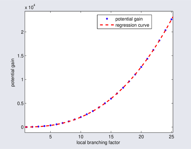
Figure 1: Plot of $PG_{10}(U)$ against $\beta$

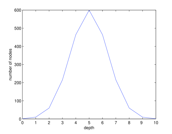
Figure 2: Plot of the distribution of $PG_{d}(U)$ for $N=10$ and $\beta=10$

4 An Alternative Discounting Factor

We next look at an alternative discounting factor. We assume that, at distance $d$ from the starting URL $U$, the user will only inspect $1/(d+1)$ of the currently available links, prior to following one of them. Thus, given $\beta$, the effective branching factor at depth $i$ is $\beta/(i+1)$ and the potential number of available nodes nodes at this depth is

$$\frac{\beta}{1}\ \frac{\beta}{2}\cdots\frac{\beta}{i}=\frac{\beta^{i}}{i!},$$ (12)

which corresponds to (1).

The alternative potential gain of $U$, denoted by $APG(U)$, is now simply the total number of available nodes at all depths, i.e.

$$APG(U)=\sum_{i=0}^{\infty}\frac{\beta^{i}}{i!}=e^{\beta},$$ (13)

which corresponds to (2). The alternative potential gain of $U$ up to depth $d$, denoted by $APG_{d}(U)$, is obtained by replacing the upper limit of the sum by $d$.

As in the case of $PG(U)$, in order to approximate $APG(U)$, we need to find the maximum depth $d$ such that

$$\frac{\beta^{d}}{d!}\geq 1.$$

By Stirling’s approximation [GKP94], $\ln(d!)\approx d\ln d-d$, so we have (approximately) that $d\leq e\beta$. Thus $\Delta=\lfloor e\beta\rfloor$.

We next consider the maximum term in the sum (13), i.e. $APG(U)$, as we did for $PG(U)$. It is straightforward to show that the maximum term is at $i=\lfloor\beta\rfloor$. Ignoring rounding errors and using Stirling’s approximation, we see that the maximum term is approximately $e^{\beta}/(2\pi{\beta})^{1/2}$. (When $\beta$ is an integer the maximum is also attained when $i=\beta-1$.)

Taking $d=\Delta=10$ we obtain the branching factor $\beta=3.6788$. In Figure 3 we show a typical plot of the alternative potential gain against the depth $d$. In this case the sum of the first $10$ terms in (13) is $39.54$, which is a good approximation of $e^{3.6788}=39.60$.

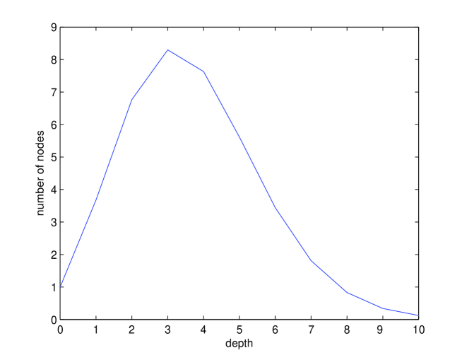
Figure 3: Plot of the distribution of $APG_{d}(U)$ for $\Delta=10$ and $\beta=3.6788$

5 Concluding Remarks

We defined a measure of navigability, called the potential gain, that provides a model of user navigation in the web. This can help the user in an online scenario to choose a starting URL for navigation, given no other information. One important factor that distinguishes the potential gain from other link analysis metrics [LM06], such as Google’s PageRank, is that it measures “hubness”, i.e. the accessibility from the page of information on others pages, rather than authority, i.e. the accessibility from elsewhere of information on the page. (See also our comment after (2) regarding another important distinction between the potential gain and PageRank.) Whereas PageRank measures authority, the Hyperlink-Induced Topic Search (HITS) algorithm [Kle99] identifies both hubs and authorities, but its computation is query-specific. In this context, it is worth noting that the potential gain is related to the notion of centrality [Fre79], which is a fundamental notion in social network analysis [Sco00].

The potential gain has been applied in a search and navigation engine that we have developed. Its distinctive feature is that an answer to a user query suggests several possible navigation paths that the user can follow [WL03], rather than just individual web pages as suggested by conventional search engines. As part of the search and navigation engine, potential gain values are pre-computed for each page in the web site being searched; these are then used to select good starting URLs for navigation [LW04].

Appendix

We obtain here the derivatives of $f(x)$. To simplify the calculations, it is convenient to let $y=\lambda(x-N/2)$ and define

$$F(y)=e^{-y^{2}}=f(x).$$

The derivatives of $f(x)$ are determined from the derivatives of $F(y)$, since

$$f^{(k)}(x)=\lambda^{k}F^{(k)}(y).$$

By straightforward differentiation we obtain:

$$F^{\prime}(y) = -2y\ e^{-y^{2}}$$

$$F^{\prime\prime}(y) = (4y^{2}-2)\ e^{-y^{2}}$$

$$F^{\prime\prime\prime}(y) = (-8y^{3}+12y)\ e^{-y^{2}}$$

$$F^{(4)}(y) = (16y^{4}-48y^{2}+12)\ e^{-y^{2}}$$

$$F^{(5)}(y) = (-32y^{5}+160y^{3}-120y)\ e^{-y^{2}}$$

These functions are closely related to the Hermite polynomials [Frö65, p.189].

We also require the extreme values of $F^{(4)}(y)$. Using a straightforward calculation, it is readily verified that the local extrema of this function are

$$F^{(4)}(y) = 12\quad\mathrm{at}\ y=0,$$

$$F^{(4)}(y) = -7.42\quad\mathrm{at}\ y=\pm((5-\sqrt{10})/2)^{1/2},$$

$$F^{(4)}(y) = 1.39\quad\mathrm{at}\ y=\pm((5+\sqrt{10})/2)^{1/2}.$$

Thus

$$-7.5<F^{(4)}(y)\leq 12.$$ (14)

References

- [AS72] M. Abramowitz and I.A. Stegun, editors. Handbook of Mathematical Functions with Formulas, Graphs and Mathematical Tables. Dover, New York, NY, 1972.
- [BBC06] R. Baeza-Yates, P. Boldi, and C. Castillo. Generalizing pagerank: damping functions for link-based ranking algorithms. In Proceedings of ACM SIGIR Conference on Research and Development in Information Retrieval, pages 308–315, Seattle, Washington, 2006.
- [Ber05] P. Berkhin. A survey on PageRank computing. Internet Mathematics, 2:73–120, 2005.
- [BGS05] M. Bianchini, M. Gori, and F. Scarselli. Inside PageRank. ACM Transactions on Internet Technology, 5:92–128, 2005.
- [BH90] F. Buckley and F. Harary. Distance in Graphs. Addison-Wesley, Redwood City, Ca., 1990.
- [DKM+02] S. Dill, R. Kumar, K. McCurley, S. Rajagopalan, D. Sivakumar, and A. Tomkins. Self-similarity in the web. ACM Transactions on Internet Technology, 2:205–223, 2002.
- [Fre79] L.C. Freeman. Centrality in social networks: Conceptual clarification. Social Networks, 1:215–239, 1979.
- [Frö65] C.-E. Fröberg. Introduction to Numerical Analysis. Addison-Wesley, Reading, Ma., 1965.
- [GKP94] R.L. Graham, D.E. Knuth, and O. Patachnik. Concrete Mathematics: A Foundation for Computer Science. Addison-Wesley, Reading, Ma., 2nd edition, 1994.
- [HPPL98] B.A. Huberman, P.L.T. Pirolli, J.E. Pitkow, and R.M. Lukose. Strong regularities in world wide web surfing. Science, 280:95–97, 1998.
- [Kle99] J.M. Kleinberg. Authoritative sources in a hyperlinked environment. Journal of the ACM, 46:604–632, 1999.
- [LBL01] M. Levene, J. Borges, and G. Loizou. Zipf’s law for web surfers. Knowledge and Information Systems, 3:120–129, 2001.
- [Lev05] M. Levene. An Introduction to Search Engines and Web Navigation. Addison-Wesley, Pearson Education, Harlow, England, 2005.
- [LL02] M. Levene and G. Loizou. Web interaction and the navigation problem in hypertext. In A. Kent, J.G. Williams, and C.M. Hall, editors, Encyclopedia of Microcomputers, pages 381–398. Marcel Dekker, New York, NY, 2002.
- [LM06] A.N. Langville and C.D. Meyer. Google’s PageRank and Beyond: The Science of Search Engine Rankings. Princeton University Press, Princeton, NJ, 2006.
- [LW04] M. Levene and R. Wheeldon. Navigating the world wide web. In M. Levene and A. Poulovassilis, editors, Web Dynamics, pages 117–151. Springer-Verlag, Berlin, 2004.
- [Nie00] J. Nielsen. Designing Web Usability: The Practice of Simplicity. New Riders Publishing, Indianapolis, Indiana, 2000.
- [Pir97] P. Pirolli. Computational models of information scent-following in a very large browsable text collection. In Proceedings of ACM Conference on Human Factors in Computing Systems, pages 3–10, Atlanta, Georgia, 1997.
- [Sco00] J. Scott. Social Network Analysis. Sage Publications, London, 2nd edition, 2000.
- [WL03] R. Wheeldon and M. Levene. The best trail algorithm for adaptive navigation in the world-wide-web. In Proceedings of the Latin American Web Congress (LA-WEB), pages 166–178, Santiago, Chile, 2003.