The tube method for the moment index in projection pursuit

Abstract

The projection pursuit index defined by a sum of squares of the third and the fourth sample cumulants is known as the moment index proposed by Jones and Sibson [14]. Limiting distribution of the maximum of the moment index under the null hypothesis that the population is multivariate normal is shown to be the maximum of a Gaussian random field with a finite Karhunen-Loève expansion. An approximate formula for tail probability of the maximum, which corresponds to the $p$-value, is given by virtue of the tube method through determining Weyl’s invariants of all degrees and the critical radius of the index manifold of the Gaussian random field.

Key words: critical radius, Euler characteristic heuristic, Hotelling-Weyl tube formula, maximum of a Gaussian random field, multiple testing, sample cumulant.

AMS 2000 subject classifications: Primary 60G15, 60G60, 62H15; secondary 53C65, 62H10.

1 Introduction

1.1 Assessing the significance in projection pursuit

Suppose that for each of $n$ individuals, a $q$ dimensional random vector $x_{t}\in{\mathbb{R}}^{q}$, $t=1,\ldots,n$, is observed as an i.i.d. sample. In the analysis of such multidimensional data, the projection of the $q$ dimensional data onto a lower dimensional subspace is often used for the sake of interpreting the data. In such cases it is important to select the subspace which clarifies features of the data interesting to the analyst. In the principal components analysis or the canonical correlation analysis, the subspaces are selected based on the variance of data ([5]). The exploratory projection pursuit is the method for detecting the subspace based on the non-normality of data ([12]). As a similar method, the Fast ICA (independent component analysis) is known ([11]).

Let ${\mathbb{S}}^{q-1}$ be a set of $q$ dimensional unit vectors, or the set of directional vectors in ${\mathbb{R}}^{q}$. In the one dimensional projection pursuit, for each directional vector $h\in{\mathbb{S}}^{q-1}$, the projection pursuit index $I_{n}(h)$ is defined as a measure for the non-normality of one dimensional projected data

$$z_{t}=\langle x_{t},h\rangle\in{\mathbb{R}},\quad t=1,\ldots,n,$$ (1.1)

and then the direction $h^{*}=\mathrm{argmax}\,I_{n}(h)$ attaining the maximum of the index is searched.

However, the index $I_{n}(h)$ is a random function of $h$ depending on the samples $x_{t}$’s. Even when $x_{t}$’s were distributed according to the multidimensional normal distribution, the function $I_{n}(h)$ is not constant, and the direction $h^{*}$ which achieves the maximum exists. Therefore, it is important to assess whether it is not a pseudo peak caused by stochastic fluctuations. For this purpose, the framework of the multiple testing can be employed. Consider the null hypothesis that the data are distributed according to the multidimensional normal distribution

$$H_{0}\,:\,x_{t}\sim N_{q}(\mu,\Sigma)\quad\rm i.i.d.,$$ (1.2)

and let

$$\bar{F}_{n}(c)=P\Bigl{(}\max_{h\in{\mathbb{S}}^{q-1}}I_{n}(h)\geq c\mid H_{0}\Bigr{)}$$

be the upper probability of the maximum of $I_{n}(h)$ under the null hypothesis. Then, $\bar{F}_{n}(I_{n}(h^{*}))$ is the $p$-value in the sense of multiple testing, and we can use the $p$-value as a measure of the significance of the maximum (Sun [20]).

Sun [20] described the limiting null distribution of the maximum of Friedman [8]’s projection pursuit index in terms of a Gaussian random field as sample size goes to infinity, and gave an approximation formula for it by an integral-geometric method referred to as the tube method ([21]). In this paper we gives an approximation formula for the moment index proposed by Jones and Sibson [14] by the tube method.

The moment index treated here is as follows: Let $K_{k,n}(h)$ be the $k$th sample cumulant of the projected data $z_{t}$ in (1.1), and let $B_{1,n}(h)=K_{3,n}(h)/K_{2,n}(h)^{3/2}$ and $B_{2,n}(h)=K_{4,n}(h)/K_{2,n}(h)^{2}$ be the sample skewness and the sample kurtosis, respectively. Then the moment index is defined by

$$I_{n}(h)=\frac{n}{6}B_{1,n}(h)^{2}+\frac{n}{24}B_{2,n}(h)^{2}.$$ (1.3)

Differently from Sun [20]’s treatment for Friedman’s index, we can determine geometric invariants of all degrees, and accordingly give an accurate formula for the $p$-values.

The structure of the paper is as follows: The main results are summarized in Section 2. There, the limiting distribution of the maximum of the moment index is described in terms of a Gaussian random field with a finite Karhunen-Loève expansion, and determine the geometric invariants of the index manifold. An approximation formula for the upper probability of the maximum can be obtained by incorporating these invariants. Some numerical experiments to examine their accuracy are given there. The main results of Section 2 are proved in Section 4. Prior to Section 4, we give a brief summary of the tube method in Section 3 as far as required.

1.2 The tube method

Here we give a very brief historical review of the tube method.

As explained in Section 3, the term tube means a spherically tubular neighborhood around a set in the sphere. Hotelling [10] pointed out a relation between the $p$-value of a testing problem in nonlinear regression and the volume of the tube, and demonstrated to calculate the $p$-value by presenting a one dimensional formula for the volume of tube. Weyl [25] generalized Hotelling [10]’s formula to the general dimensional case. More recently, Knowles and Siegmund [15] and Sun [21] found out the relation between the formula for the volume of tube and the tail probability formula for the maximum of a Gaussian random field. Since then, the tube method was applied to statistical problems such as calculating null distributions of max-type test statistics, or adjusting the multiplicity in multiple testing problems. For example, the asymptotic distribution of the Anderson-Stephens statistic ([6]) for testing the uniformity of direction can be evaluated ([18]). For the other examples, see [17] and [16]. Nowadays, the tube method was proved by Takemura and Kuriki [22] to be a special case of the Euler characteristic heuristics, which is known as another approach for approximating the distribution of the maxima of random fields developed by Adler ([2], [3]), Worsley ([26], [27]) and Taylor ([23]). For recent developments of the tube method and the Euler characteristic heuristic, see Adler and Taylor [4]. See also [19].

2 Main results

We begin with giving the limiting distribution of the moment index $I_{n}(h)$ in (1.3) under the null hypothesis of multivariate normality. Without loss of generality, we assume that $x_{t}$’s are distributed according to the $q$ dimensional standard normal distribution $N_{q}(0,I_{q})$.

Theorem 2.1

Let $\xi_{1}\in{\mathbb{R}}^{q^{3}}$, $\xi_{2}\in{\mathbb{R}}^{q^{4}}$ be random vectors consisting of independent standard normal random variables. For a unit vector $h\in{\mathbb{S}}^{q-1}$, let

$$Z_{1}(h)=\langle h\otimes h\otimes h,\xi_{1}\rangle,\quad Z_{2}(h)=\langle h\otimes h\otimes h\otimes h,\xi_{2}\rangle,$$ (2.1)

where $\otimes$ denotes the Kronecker product. Under the null hypothesis $H_{0}$ in (1.2), as $n\to\infty$, $\max_{h\in{\mathbb{S}}^{q-1}}I_{n}(h)$ converges in distribution to $\max_{h\in{\mathbb{S}}^{q-1}}I(h)$, where

$$I(h)=Z_{1}(h)^{2}+Z_{2}(h)^{2}.$$

Proof.

Let $C({\mathbb{S}}^{q-1})$ be the Banach space of real valued continuous functions on ${\mathbb{S}}^{q-1}$ endowed with the supremum norm. Note that the sample cumulant $K_{k,n}(\cdot)$, the sample skewness $B_{1,n}(\cdot)$, the kurtosis $B_{2,n}(\cdot)$, and the moment index $I_{n}(\cdot)$ are the elements of $C({\mathbb{S}}^{q-1})$. Theorem 2.1 of Kuriki and Takemura [17] states that the $(\sqrt{n}B_{1,n}(\cdot),\sqrt{n}B_{2,n}(\cdot))$ converges to $(\sqrt{3!}Z_{1}(\cdot),\sqrt{4!}Z_{2}(\cdot))$ in distribution in the space $C({\mathbb{S}}^{q-1})$. The theorem follows from the continuous mapping theorem.  

∎

By means of Theorem 2.1 above, for large sample size $n$, the $p$-value $\bar{F}_{n}(I_{n}(h^{*}))$ can be approximated by $\bar{F}(I_{n}(h^{*}))$ with

$$\bar{F}(c)=P\Bigl{(}\max_{h\in{\mathbb{S}}^{q-1}}I(h)\geq c\Bigr{)}.$$

Moreover, by letting

$$Z(h,\theta)=\cos\theta Z_{1}(h)+\sin\theta Z_{2}(h),\quad h\in{\mathbb{S}}^{q-1},\ \theta\in\Bigl{(}-\frac{\pi}{2},\frac{\pi}{2}\Bigr{]}$$

with $Z_{1}(h)$ and $Z_{2}(h)$ given in (2.1), we have

$$\Bigl{\{}\max_{h\in{\mathbb{S}}^{q-1}}I(h)\Bigr{\}}^{1/2}=\max_{h\in{\mathbb{S}}^{q-1},\,\theta\in(-\pi/2,\pi/2]}Z(h,\theta).$$ (2.2)

Therefore, from now on, we restrict our attention to the distribution of the maximum of $Z(h,\theta)$.

Let

$$p=q^{3}+q^{4}$$

and

$$M=\left\{(\cos\theta(h\otimes h\otimes h),\sin\theta(h\otimes h\otimes h\otimes h))\in{\mathbb{R}}^{p}\mid h\in{\mathbb{S}}^{q-1},\ \theta\in\Bigr{(}-\frac{\pi}{2},\frac{\pi}{2}\Bigl{]}\right\}.$$ (2.3)

The maximum (2.2) can be rewritten as

$$\max_{x\in M}\langle x,\xi\rangle,\qquad\xi=(\xi_{1},\ldots,\xi_{p})\sim N_{p}(0,I_{p}).$$ (2.4)

Note that $M$ and ${\mathbb{S}}^{q-1}\times(-\pi/2,\pi/2]$ are one-to-one. It is easy to see that $M$ is a $q$ dimensional closed submanifold of ${\mathbb{S}}^{p-1}$. As shall be explained in Section 3, (2.4) is of the canonical form of the tube method in (3.1).

The upper probability function of the chi-square distribution with $\nu$ degrees of freedom is denoted by

$$\bar{G}_{\nu}(c)=\frac{1}{2^{\nu/2}\Gamma(\nu/2)}\int_{c}^{\infty}t^{\nu/2-1}e^{-t/2}dt.$$ (2.5)

The volume of the $m-1$ dimensional volume of the unit sphere ${\mathbb{S}}^{m-1}$ is denoted by

$$\Omega_{m}=\frac{2\pi^{m/2}}{\Gamma(m/2)}.$$ (2.6)

The following is the main theorem of this paper. The proof is given in Sections 4.1 and 4.2.

Theorem 2.2

As $c\to\infty$,

$$P\Bigl{(}\max_{h\in{\mathbb{S}}^{q-1}}I(h)\geq c^{2}\Bigr{)}=\sum_{e=0,\,e:{\rm even}}^{q}\kappa_{e}\frac{\Gamma((q+1-e)/2)}{2^{1+e/2}\pi^{(q+1)/2}}\bar{G}_{q+1-e}(c^{2})+O\bigl{(}c^{p-2}e^{-\rho_{c}c^{2}/2}\bigr{)},$$

where

$$\kappa_{e}=\Omega_{q}\,\frac{(-3)^{e/2}(q-1)!}{(q-e)!}\sum_{j=0}^{e/2}\frac{(q-e-2j)}{(e/2-j)!\,j!}(-2)^{j}E_{(q-1-e)/2-j},$$ (2.7)

$$E_{k}=\int_{-\pi/2}^{\pi/2}(3\cos^{2}\theta+4\sin^{2}\theta)^{k}d\theta$$ (2.8)

and

$$\rho_{c}=\frac{25}{16}.$$ (2.9)

Remark 2.1

$E_{k}$ in (2.8) with $k$ an integer or a half-integer can be evaluated numerically by recurrence formulas:

$$E_{k}=\frac{7(2k-1)}{2k}E_{k-1}-\frac{12(k-1)}{k}E_{k-2},\quad\mbox{for\ \ }k=1,\frac{3}{2},2,\ldots,$$ (2.10)

and

$$E_{k}=\frac{7(2k+3)}{24(k+1)}E_{k+1}-\frac{k+2}{12(k+1)}E_{k+2},\quad\mbox{for\ \ }k=-\frac{3}{2},-2,-\frac{5}{2},\ldots,$$ (2.11)

with the boundary conditions

$$E_{1/2}=4E(1/4)\doteq 4\times 1.46746,\quad E_{0}=\pi,\quad E_{-1/2}=K(1/4)\doteq 1.68575,\quad E_{-1}=\frac{\pi}{2\sqrt{3}},$$

where $E(1/4)$ and $K(1/4)$ are complete elliptic integrals of the first kind and the second kind ([1], p. 608–9). The proofs for (2.10) and (2.11) are given in Section 4.3.

To conclude this section, we give numerical examples for the purpose of examining the accuracy of the formula. The tail probability of the maximum for $q=2$ is given by

$$P\Bigl{(}\max_{h\in{\mathbb{S}}^{2-1}}I(h)\geq c^{2}\Bigr{)}\,\sim\,w\bigl{\{}\bar{G}_{3}(c^{2})-\bar{G}_{1}(c^{2})\bigr{\}}\,=\,w\sqrt{\frac{2}{\pi}}\,c\,e^{-c^{2}/2},\qquad c\to\infty,$$ (2.12)

where $w=2E(1/4)\doteq 2\times 1.46746$.

Figure 1 depicts the empirical upper probability of the limiting distribution $P(\max_{h\in{\mathbb{S}}^{2-1}}I(h)\allowbreak\geq x)$ estimated by Monte Carlo simulations based on 10,000 replications, and its approximation by the tube method. One can see that the quantiles of the limiting distribution are fully approximated by the tube method approximation (2.12).

Figure 2 depicts the empirical upper probability of the finite sample distributions $P(\max_{h\in{\mathbb{S}}^{2-1}}\allowbreak I_{n}(h)\geq x)$ when $n=300,1000,3000,\infty$. The number of replications is 10,000.

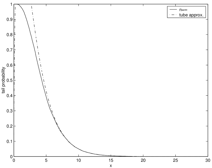
Figure 1: Tail probability of limiting distribution (solid line) and its approximation by the tube method (dotted line).

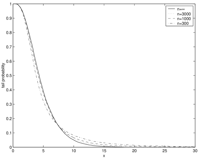
Figure 2: Tail probabilities of finite sample distributions ($n=300,1000,3000,\infty$).

3 Summary of the tube method

3.1 Volume of the tubes and tail probabilities of the maxima

In this section we summarize the facts on the tube method required for proving Theorem 2.2. We state Theorem 3.1 since its statement is not given in existing literature.

Let ${\mathbb{S}}^{p-1}$ be the unit sphere in ${\mathbb{R}}^{p}$, and let $M$ be a closed subset of ${\mathbb{S}}^{p-1}$. Assume that $M$ is a $d$ dimensional $C^{2}$ closed submanifold without boundaries embedded in ${\mathbb{S}}^{p-1}$, and is endowed with the metric induced by the standard inner product $\langle\cdot,\cdot\rangle$ of ${\mathbb{R}}^{p}$.

The set of points of ${\mathbb{S}}^{p-1}$ whose great circle distance (angle) from $M$ is less than or equal to a constant $\theta$ is called the tube about $M$ with the radius $\theta$, and denoted by

$$\mathrm{Tube}(M,\theta)=\Big{\{}y\in{\mathbb{S}}^{p-1}\mid\mathrm{dist}(y,M)\leq\theta\Big{\}},\qquad\mathrm{dist}(y,M)=\min_{x\in M}\ \cos^{-1}\langle y,x\rangle.$$

In a similar manner, the Euclidean tube is defined in the Euclidean space by the usual distance. But it does not play any role in this paper.

Let $y$ be a point of ${\mathbb{S}}^{p-1}\setminus M$. The point $x=\mathrm{pr}(y)$ which attains the minimum $\min_{x\in M}\mathrm{dist}(y,x)$ is called the projection of $y$ onto $M$. If $y$ is close to $M$, then $\mathrm{pr}(y)$ exists uniquely. Whereas, if $y$ is far from $M$, then there can exist two points $x_{1},x_{2}\in M$ equidistant from $y$ which attain the minimum $\min_{x\in M}\mathrm{dist}(y,x)$ simultaneously. The supremum of the distances which assures the uniqueness is called the critical radius.

Definition 3.1

When the $\mathrm{pr}(y)\in M$ is defined uniquely for every $y\in\mathrm{Tube}(M,\theta)\setminus M$, it is said that the tube $\mathrm{Tube}(M,\theta)$ does not have a self-overlap. The supremum

$$\theta_{c}=\sup\{\theta\geq 0\mid\mbox{$\mathrm{Tube}(M,\theta)$ does not have a self-overlap}\}$$

is called the critical radius of $M$.

The volume of a tube whose radius is less than or equal to the critical radius $\theta_{c}$ can be calculated by taking a coordinate system based on the projection (the Fermi coordinates). The following proposition for the dimension $d=1$ is due to Hotelling [10], and due to Weyl [25] for the general dimensional case. Here $\Omega_{p}$ denotes the $p-1$ dimensional volume of ${\mathbb{S}}^{p-1}$ defined in (2.6), and

$$\bar{B}_{a,b}(c)=\frac{\Gamma(a+b)}{\Gamma(a)\Gamma(b)}\int_{c}^{1}t^{a-1}(1-t)^{b-1}dt$$

is the upper probability function of the beta distribution with parameters $(a,b)$.

Proposition 3.1

For $0\leq\theta\leq\theta_{c}$, $p-1$ dimensional volume of the tube is given by

$$\mathrm{Vol}(\mathrm{Tube}(M,\theta))=\Omega_{p}\sum_{e=0,\ e:\,\rm even}^{d}\kappa_{e}J_{e}(\theta),$$

where

$$J_{e}(\theta)=\frac{\Gamma((d+1-e)/2)}{2^{1+e/2}\pi^{(d+1)/2}}\bar{B}_{(d+1-e)/2,(p-d-1+e)/2}(\cos^{2}\theta),$$

and the $\kappa_{e}$ is the intrinsic invariant of the manifold $M$ defined below in (3.6), referred to as Weyl’s curvature invariant.

Let $\xi=(\xi_{1},\ldots,\xi_{p})$ be a random vector consisting of independent standard normal random variables. That is, $\xi\sim N_{p}(0,I_{p})$. Define a Gaussian random field on a submanifold $M$ of ${\mathbb{S}}^{p-1}$ by

$$Z(x)=\langle x,\xi\rangle,\quad x\in M\ \ (\subset{\mathbb{S}}^{p-1}).$$ (3.1)

This is a canonical form of Gaussian random fields of mean 0 and variance 1 with a finite Karhunen-Loève expansion.

By replacing $\Omega_{p}\bar{B}$ by the upper probability function of the chi-square distribution $\bar{G}$ in (2.5), we have an approximation formula for the tail probability of the maximum of $Z(x)$ ([17], [22]).

Proposition 3.2

As $c\to\infty$,

$$P\Bigl{(}\max_{x\in M}Z(x)\geq c\Bigr{)}=\sum_{e=0,\,e:\rm even}^{d}\kappa_{e}\psi_{e}(c)+O\bigl{(}c^{p-2}e^{-(1+\tan^{2}\theta_{c})c^{2}/2}\bigr{)},$$

where

$$\psi_{e}(c)=\frac{\Gamma((d+1-e)/2)}{2^{1+e/2}\pi^{(d+1)/2}}\bar{G}_{d+1-e}(c^{2}).$$

Note that the larger the critical radius $\theta_{c}$ is, the smaller the order of the remainder term is.

3.2 Weyl’s curvature invariants

As we saw in Propositions 3.1 and 3.2, the Weyl’s curvature invariants $\kappa_{e}$ and the critical radius $\theta_{c}$ of the manifold $M$ are needed in applying the tube method. We will explain the way to determine them in this and subsequent subsections.

Write a local coordinate system of a $d$ dimensional closed manifold $M$ as $(t^{i})$. The metric tensor is denoted by $g_{ij}$, and write the $(i,j)$th elements of the inverse of the $d\times d$ matrix $(g_{ij})$ as $g^{ij}$. Abbreviate $\partial/\partial t^{i}$ to $\partial_{i}$. The connection coefficients and the curvature tensor are given by

$$\Gamma_{ij}^{k}=\sum_{h=1}^{d}g^{kh}\Gamma_{ij,h}\quad\mbox{with}\quad\Gamma_{ij,k}=\frac{1}{2}(\partial_{i}g_{jk}+\partial_{j}g_{ik}-\partial_{k}g_{ij}),$$ (3.2)

and

$$R^{kl}_{ij}=\sum_{h}g^{lh}{R^{k}}_{hij}\quad\mbox{with}\quad{R^{l}}_{kij}=\partial_{i}\Gamma^{l}_{jk}-\partial_{j}\Gamma^{l}_{ik}+\sum_{s=1}^{d}(\Gamma^{l}_{is}\Gamma^{s}_{jk}-\Gamma^{l}_{js}\Gamma^{s}_{ik}),$$ (3.3)

respectively. Let

$$H^{kl}_{ij}=R^{kl}_{ij}-(\delta^{k}_{i}\delta^{l}_{j}-\delta^{l}_{i}\delta^{k}_{j}),$$ (3.4)

where $\delta_{i}^{j}$ is Kronecker’s delta. For $e=0,2,\ldots,[d/2]\times 2$, let

$$H_{e}=\sum_{i}\sum_{\sigma}\mathrm{sgn}(\sigma)\,H_{i_{1}i_{2}}^{i_{\sigma(1)}i_{\sigma(2)}}H_{i_{3}i_{4}}^{i_{\sigma(3)}i_{\sigma(4)}}\cdots H_{i_{e-1}i_{e}}^{i_{\sigma(e-1)}i_{\sigma(e)}}.$$ (3.5)

Here the summation $\sum_{i}$ is taken over all sets of $e/2$ paring made of distinct elements of $\{1,2,\ldots,d\}$, that is, all possible ways of $\{i_{1},i_{2},\ldots,i_{e}\}\subset\{1,2,\ldots,d\}$ satisfying $i_{1}<i_{2}$, $i_{3}<i_{4},\ldots,i_{e-1}<i_{e}$ and $i_{1}<i_{3}<\cdots<i_{e-1}$. The summation $\sum_{\sigma}$ is taken over all permutations $\sigma$ of $\{1,2,\ldots,e\}$ such that $\sigma(1)<\sigma(2)$, $\sigma(3)<\sigma(4),\ldots,\sigma(e-1)<\sigma(e)$. Then, Weyl’s curvature invariants are defined by

$$\kappa_{e}=\int_{M}H_{e}\,\det(g_{ij})^{1/2}dt^{1}\cdots dt^{d},\qquad e=0,2,\ldots,[d/2]\times d$$ (3.6)

(Weyl [25]).

For instance, $H_{e}$ for $e=0,2,4$ are given as follows: $H_{0}=1$, and hence $\kappa_{0}$ is the $d$ dimensional volume of $M$.

$$H_{2}=\sum_{1\leq i<j\leq d}H^{ij}_{ij}=\frac{1}{2}\sum_{i,j=1}^{d}H^{ij}_{ij}=\frac{1}{2}\Bigl{\{}\sum_{i,j=1}^{d}R^{ij}_{ij}-d(d-1)\Bigr{\}},$$

where $\sum_{i,j=1}^{d}R^{ij}_{ij}$ is the scalar curvature.

$$H_{4} = \sum_{1\leq i<j<k<l\leq d}(H_{ij}^{ij}H_{kl}^{kl}-H_{ij}^{ik}H_{kl}^{jl}+H_{ij}^{il}H_{kl}^{jk}+H_{ij}^{jk}H_{kl}^{il}-H_{ij}^{jl}H_{kl}^{ik}+H_{ij}^{kl}H_{kl}^{ij}$$

$$\qquad\qquad\quad-H_{ik}^{ij}H_{jl}^{kl}+H_{ik}^{ik}H_{jl}^{jl}-H_{ik}^{il}H_{jl}^{jk}-H_{ik}^{jk}H_{jl}^{il}+H_{ik}^{jl}H_{jl}^{ik}-H_{ik}^{kl}H_{jl}^{ij}$$

$$\qquad\qquad\quad+H_{il}^{ij}H_{jk}^{kl}-H_{il}^{ik}H_{jk}^{jl}+H_{il}^{il}H_{jk}^{jk}+H_{il}^{jk}H_{jk}^{il}-H_{il}^{jl}H_{jk}^{ik}+H_{il}^{kl}H_{jk}^{ij})$$

$$= \frac{1}{8}\sum_{i,j,k,l=1}^{d}(H_{ij}^{ij}H_{kl}^{kl}-4H_{ij}^{il}H_{kl}^{kj}+H_{ij}^{kl}H_{kl}^{ij})$$

$$= \frac{1}{8}\Bigl{\{}\Bigl{(}\sum_{i,j=1}^{d}R_{ij}^{ij}\Bigr{)}^{2}-4\sum_{i,j,k,l=1}^{d}R_{ij}^{il}R_{kl}^{kj}+\sum_{i,j,k,l=1}^{d}R_{ij}^{kl}R_{kl}^{ij}$$

$$\qquad\quad-2(d-2)(d-3)\sum_{i,j=1}^{d}R_{ij}^{ij}+d(d-1)(d-2)(d-3)\Bigr{\}}.$$

See Gray ([9], Lemma 4.2) for the invariants of a Euclidean tube.

3.3 Evaluation of critical radius

In this subsection we give theorems useful in calculating the critical radius of a closed submanifold of the sphere.

Proposition 3.3

The critical radius $\theta_{c}$ of a closed submanifold $M$ of ${\mathbb{S}}^{p-1}$ satisfies

$$\cot^{2}\theta_{c}=\sup_{y,x\in M,\,y\neq x}h(x,y),\qquad h(x,y)=\frac{1-\langle y,P_{x}y\rangle}{(1-\langle x,y\rangle)^{2}},$$ (3.7)

where $P_{x}$ is the orthogonal projection onto the linear subspace $\mathrm{span}\{x\}\oplus T_{x}M$ of ${\mathbb{R}}^{p}$, and $T_{x}M$ is the tangent space of $M$ at $x$ ([13], [17]).

A theorem corresponding to a Euclidean tube is given by Federer ([7], Theorem 4.18).

The radius $\theta_{c}^{\rm loc}$ satisfying

$$\cot^{2}\theta_{c}^{\rm loc}=\limsup_{y,x\in M,\,\|y-x\|\to 0}h(x,y)$$ (3.8)

is called the local critical radius, which is characterized as the curvature radius of $M$ at $x$ ([13], [17]). By definitions, $\theta_{c}^{\rm loc}\geq\theta_{c}$, and the equality holds if the supremum in (3.7) is attained when $\|y-x\|\to 0$.

Define a real-valued function on $M\times M$ by $r(x,y)=\langle x,y\rangle$. This is the covariance function of the Gaussian random field (3.1). Denote the local coordinate system about $x$ and $y$ by $(s^{i})$, $(t^{i})$, respectively.

The set of the critical points of $r(x,y)$ which are not contained in the diagonal set is denoted by

$$C=\Bigl{\{}(x,y)\in M\times M\mid x\neq y,\ \frac{\partial}{\partial s^{i}}r(x,y)=0,\ \frac{\partial}{\partial t^{i}}r(x,y)=0\Bigr{\}}.$$

Then we have the following theorem.

Theorem 3.1

The critical radius $\theta_{c}$ satisfies

$$\theta_{c}=\min\Bigl{\{}\theta_{c}^{\rm loc},\inf_{(x,y)\in C}\frac{1}{2}\cos^{-1}\langle x,y\rangle\Bigr{\}}.$$

Proof.

By Lemma 5.2 of [24], if the supremum of $h(x,y)$ is attained at a point not contained in the diagonal set, then it belongs to $C$. Furthermore, for the points $(x,y)\in C$, it holds that $P_{x}y=\langle x,y\rangle x$,

$$h(x,y)=\frac{1-\langle x,y\rangle^{2}}{(1-\langle x,y\rangle)^{2}}=\frac{1+\langle x,y\rangle}{1-\langle x,y\rangle}=\cot^{2}\Bigl{(}\frac{1}{2}\cos^{-1}\langle x,y\rangle\Bigr{)},$$

and hence

$$\sup_{(x,y)\in C}h(x,y)=\cot^{2}\Bigl{(}\inf_{(x,y)\in C}\frac{1}{2}\cos^{-1}\langle x,y\rangle\Bigr{)}.$$

Since the supremum of $h(x,y)$ over the diagonal set is $\cot^{2}\theta_{c}^{\rm loc}$, the theorem follows from Proposition 3.3.  

∎

A theorem corresponding to a Euclidean tube with the dimension $d=1$ is given by Johansen and Johnstone ([13], Proposition 4.2).

4 Proof of Theorem 2.2

4.1 Proof of (2.7)

In this section, we prove Theorem 2.2. By means of Proposition 3.2, the approximation formula for the upper probability of the maximum can be given through determining Weyl’s curvature invariants $\kappa_{e}$ and the critical radius $\theta_{c}$ of the index manifold $M$ in (2.3). The former is given here, and the latter is given in the next subsection.

The metric tensor, the connection coefficients, and the curvature tensor for $M$ are denoted by $g$, $\Gamma$, and $R$, respectively, as in Section 3.2. Also, the same quantities for ${\mathbb{S}}^{q-1}$ are denoted by $\bar{g}$, $\bar{\Gamma}$, and $\bar{R}$, respectively.

Write an element $h$ of ${\mathbb{S}}^{q-1}$ by a local coordinate system as $h=h(t)$, $t=(t^{i})$. Let $h_{i}=\partial h/\partial t^{i}$. The metric of ${\mathbb{S}}^{q-1}$ is $\bar{g}_{ij}=\langle h_{i},h_{j}\rangle$.

An element $x$ of $M$ can be written as

$$x=(\cos\theta(h\otimes h\otimes h),\sin\theta(h\otimes h\otimes h\otimes h))\in M$$

in terms of $(t,\theta)$. The bases of the tangent space of $M$ are

$$\frac{\partial x}{\partial t^{i}}=(\cos\theta(h_{i}\otimes h\otimes h+h\otimes h_{i}\otimes h+h\otimes h\otimes h_{i}),$$

$$\qquad\quad\ \sin\theta(h_{i}\otimes h\otimes h\otimes h+h\otimes h_{i}\otimes h\otimes h+h\otimes h\otimes h_{i}\otimes h$$

$$\qquad\qquad\qquad\qquad+h\otimes h\otimes h\otimes h_{i})),\quad i=1,\ldots,q-1,$$

$$\frac{\partial x}{\partial\theta}=(-\sin\theta(h\otimes h\otimes h),\cos\theta(h\otimes h\otimes h\otimes h\otimes h)).$$

In the following, $\theta$ is regarded as the 0th coordinate $t^{0}$ of $t$. The metric tensor of $M$ is

$$g_{ij}=\begin{cases}v(\theta)\bar{g}_{ij}(t)&\mbox{if $i,j\neq 0$},\\ 1&\mbox{if $i=j=0$},\\ 0&\mbox{otherwise},\end{cases}$$

where

$$v(\theta)=3\cos^{2}\theta+4\sin^{2}\theta=3+\sin^{2}\theta=4-\cos^{2}\theta.$$ (4.1)

From this, the volume element of $M$ is shown to be

$$\det(\bar{g}_{ij}(t))^{1/2}dt^{1}\cdots dt^{q-1}\,v(\theta)^{(q-1)/2}\,d\theta.$$ (4.2)

Note that $\det(\bar{g}_{ij}(t))^{1/2}dt^{1}\cdots dt^{q-1}$ is the volume element of ${\mathbb{S}}^{q-1}$.

Let $\dot{v}$ and $\ddot{v}$ be the first and second derivatives of $v=v(\theta)$. After some calculations along the lines with (3.2), it is shown that the non-zero connection coefficients of $M$ are

$$\Gamma_{ij}^{k}=\bar{\Gamma}_{ij}^{k},\qquad\Gamma_{i0}^{k}=\Gamma_{0i}^{k}=\frac{1}{2}\frac{\dot{v}}{v}\delta_{i}^{k},\qquad\Gamma_{ij}^{0}=-\frac{1}{2}\dot{v}\bar{g}_{ij}\qquad(i,j,k\neq 0),$$

and all of the other coefficients are 0.

Next we will derive the curvature tensor by (3.3). Put

$$J^{kl}_{ij}=\delta^{k}_{i}\delta^{l}_{j}-\delta^{l}_{i}\delta^{k}_{j}.$$

Noting that the curvature tensor of the unit sphere ${\mathbb{S}}^{q-1}$ is $\bar{R}^{kl}_{ij}=J^{kl}_{ij}$, after cumbersome calculations we see that the non-zero elements are

$$R^{kl}_{ij}=\Bigl{\{}\frac{1}{v}-\frac{1}{4}\Bigl{(}\frac{\dot{v}}{v}\Bigr{)}^{2}\Bigr{\}}J^{kl}_{ij},\qquad R^{k0}_{i0}=-R^{0k}_{i0}=-R^{k0}_{0i}=R^{0k}_{0i}=\Bigl{\{}-\frac{1}{2}\frac{\ddot{v}}{v}+\frac{1}{4}\Bigl{(}\frac{\dot{v}}{v}\Bigr{)}^{2}\Bigr{\}}\delta^{k}_{i}\qquad(i,j,k,l\neq 0).$$

Furthermore, noting that $\dot{v}=2\cos\theta\sin\theta$, $(\dot{v})^{2}=4\cos^{2}\theta\sin^{2}\theta=4(4-v)(v-3)=-4(v^{2}-7v+12)$, $\ddot{v}=2\cos^{2}\theta-2\sin^{2}\theta=2(4-v)-2(v-3)=-2(2v-7)$, we have the non-zero elements of $H^{kl}_{ij}$ in (3.4) as

$$H^{kl}_{ij}=\alpha J^{kl}_{ij},\qquad H^{k0}_{i0}=-H^{0k}_{i0}=-H^{k0}_{0i}=H^{0k}_{0i}=\beta\delta^{k}_{i}\qquad(i,j,k,l\neq 0),$$

where

$$\alpha=\alpha(\theta)=-\frac{6}{v}+\frac{12}{v^{2}},\qquad\beta=\beta(\theta)=-\frac{12}{v^{2}}.$$

We substitute these quantities into (3.5) to obtain $H_{e}$, $e=0,2,\ldots,[q/2]\times 2$.

(i)  The case where the set of the indices $i_{1},i_{2},\ldots,i_{e}$ in the right-hand side of (3.5) does not contain 0. Because the number of the ways to make $e/2$ pairs from $q-1$ distinct objects is

$$\frac{(q-1)!}{(q-1-e)!2^{e/2}(e/2)!},$$

the summation of all terms corresponding to the case (i) becomes

$$\alpha^{e/2}\times\frac{(q-1)!}{(q-1-e)!2^{e/2}(e/2)!}.$$ (4.3)

(ii)  The case where the set of the indices $i_{1},i_{2},\ldots,i_{e}$ in the right-hand side of (3.5) contains 0. In this case, $i_{1}=0$, and $i_{2}\neq 0$, $\sigma(1)=1$ ($i_{\sigma(1)}=0$). Noting that there are $q-1$ ways for $i_{2}$ ($i_{2}=1,\ldots,q-1$), and that $i_{3},i_{4},\ldots,i_{e}$ are indices resulting from making $e/2-1$ pairs from the set $\{1,2,\dots,q-1\}\setminus\{i_{2}\}$ having $q-2$ elements, the summation of all terms corresponding to the case (ii) becomes

$$(q-1)\beta\alpha^{e/2-1}\times\frac{(q-2)!}{(q-e)!2^{e/2-1}(e/2-1)!}.$$ (4.4)

Summing up (4.3) and (4.4) along with

$$\alpha^{e/2}=\Bigl{(}-\frac{6}{v}\Bigr{)}^{e/2}\sum_{j=0}^{e/2}{e/2\choose j}\Bigl{(}-\frac{2}{v}\Bigr{)}^{j}$$

and

$$\beta\alpha^{e/2-1}=-\Bigl{(}-\frac{6}{v}\Bigr{)}^{e/2}\sum_{j=1}^{e/2}{e/2-1\choose j-1}\Bigl{(}-\frac{2}{v}\Bigr{)}^{j}$$

yields

$$H_{e}=\sum_{j=0}^{e/2}\frac{A_{j}}{v^{e/2+j}},$$

where

$$A_{0}=\frac{(-3)^{e/2}(q-1)!}{(q-e-1)!(e/2)!},$$

and for $j\neq 0$,

$$A_{j} = (-6)^{e/2}(-2)^{j}\biggl{\{}\frac{(q-1)!}{(q-1-e)!2^{e/2}(e/2)!}{e/2\choose j}-\frac{(q-1)(q-2)!}{(q-e)!2^{e/2-1}(e/2-1)!}{e/2-1\choose j-1}\biggr{\}}$$

$$= \frac{(-3)^{e/2}(q-1)!}{(q-e)!}\frac{(q-e+2j)(-2)^{j}}{(e/2-j)!j!}.$$

Since the expression for $A_{j}$ with $j\neq 0$ is consistent with that for $A_{0}$, we have

$$H_{e}=\frac{(-3)^{e/2}(q-1)!}{(q-e)!}\sum_{j=0}^{e/2}\frac{(q-e-2j)(-2)^{j}}{(e/2-j)!j!}\frac{1}{v^{e/2+j}}.$$

Finally we obtain $\kappa_{e}$ in (2.7) by integrating $H_{e}$ over $M$ with respect to the volume element (4.2).

4.2 Proof of (2.9)

In this subsection, making use of Theorem 3.1, we show that the critical radius of the index manifold $M$ in (2.3) is $\theta_{c}=\tan^{-1}(3/4)$. This implies that $\rho_{c}=1+\tan^{2}\theta_{c}=25/16$. Throughout this subsection, we assume that vectors are column vectors for notational convenience. For instance, $\langle x,y\rangle=x^{\prime}y$, where ^′ denotes the transpose.

We begin with obtaining the local critical radius $\theta_{c}^{\rm loc}$ by (3.8). Let

$$x=\begin{pmatrix}\cos\theta(h\otimes h\otimes h)\\ \sin\theta(h\otimes h\otimes h\otimes h)\end{pmatrix},\qquad{\tilde{x}}=\begin{pmatrix}\cos{\tilde{\theta}}({\tilde{h}}\otimes{\tilde{h}}\otimes{\tilde{h}})\\ \sin{\tilde{\theta}}({\tilde{h}}\otimes{\tilde{h}}\otimes{\tilde{h}}\otimes{\tilde{h}})\end{pmatrix}$$

be two points of $M$. Write for simplicity $h_{i}=\partial h/\partial t^{i}$, $x_{i}=\partial x/\partial t^{i}$, $x_{0}=\partial x/\partial\theta$, and $\bar{G}=(\bar{g}_{ij})$, $v=v(\theta)$ defined in (4.1). The orthogonal projection matrix onto $\mathrm{span}\{x\}\oplus T_{x}M$ is denoted by $P_{x}$. Since $\mathrm{span}\{x\}$ is orthogonal to $T_{x}M$, we have

$${\tilde{x}}^{\prime}P_{x}{\tilde{x}} = ({\tilde{x}}^{\prime}x,{\tilde{x}}^{\prime}x_{1},\ldots,{\tilde{x}}^{\prime}x_{q-1},{\tilde{x}}^{\prime}x_{0})\begin{pmatrix}1&&\\ &v\bar{G}&\cr&&1\end{pmatrix}^{-1}\begin{pmatrix}{\tilde{x}}^{\prime}x\\ {\tilde{x}}^{\prime}x_{1}\\ \vdots\\ {\tilde{x}}^{\prime}x_{q-1}\\ {\tilde{x}}^{\prime}x_{0}\end{pmatrix}$$

$$= ({\tilde{x}}^{\prime}x)^{2}+({\tilde{x}}^{\prime}x_{1},\ldots,{\tilde{x}}^{\prime}x_{q-1})(v\bar{G})^{-1}\begin{pmatrix}{\tilde{x}}^{\prime}x_{1}\cr\vdots\\ {\tilde{x}}^{\prime}x_{q-1}\end{pmatrix}+({\tilde{x}}^{\prime}x_{0})^{2}.$$

The first term of the right-hand side is the square of

$${\tilde{x}}^{\prime}x=({\tilde{h}}^{\prime}h)^{3}\cos{\tilde{\theta}}\cos\theta+({\tilde{h}}^{\prime}h)^{4}\sin{\tilde{\theta}}\sin\theta.$$

Noting that

$${\tilde{x}}^{\prime}x_{i}=w{\tilde{h}}^{\prime}h_{i},\qquad w=3({\tilde{h}}^{\prime}h)^{2}\cos{\tilde{\theta}}\cos\theta+4({\tilde{h}}^{\prime}h)^{3}\sin{\tilde{\theta}}\sin\theta,$$

the second term becomes

$$\frac{w^{2}}{v}\,{\tilde{h}}^{\prime}(h_{1},\ldots,h_{q-1})\bar{G}^{-1}\begin{pmatrix}h_{1}^{\prime}\\ \vdots\\ h_{q-1}^{\prime}\end{pmatrix}{\tilde{h}}^{\prime}=\frac{w^{2}}{v}\,{\tilde{h}}^{\prime}(I_{q}-hh^{\prime}){\tilde{h}}=\frac{w^{2}}{v}\,(1-({\tilde{h}}^{\prime}h)^{2}).$$

The third term is the square of

$${\tilde{x}}^{\prime}x_{0}=-({\tilde{h}}^{\prime}h)^{3}\cos{\tilde{\theta}}\sin\theta+({\tilde{h}}^{\prime}h)^{4}\sin{\tilde{\theta}}\cos\theta.$$

Summing up these three terms, the numerator of the right-hand side of (3.8) is

$$1-{\tilde{x}}^{\prime}P_{x}{\tilde{x}} = 1-(({\tilde{h}}^{\prime}h)^{3}\cos{\tilde{\theta}}\cos\theta+({\tilde{h}}^{\prime}h)^{4}\sin{\tilde{\theta}}\sin\theta)^{2}-\frac{w^{2}}{v}\,(1-({\tilde{h}}^{\prime}h)^{2})$$

$$-(-({\tilde{h}}^{\prime}h)^{3}\cos{\tilde{\theta}}\sin\theta+({\tilde{h}}^{\prime}h)^{4}\sin{\tilde{\theta}}\cos\theta)^{2}$$

$$= 1-\cos^{6}\psi\cos^{2}\tilde{\theta}-\cos^{8}\psi\sin^{2}\tilde{\theta}$$

$$-\frac{(3\cos^{2}\psi\cos\tilde{\theta}\cos\theta+4\cos^{3}\psi\sin\tilde{\theta}\sin\theta)^{2}}{3\cos^{2}\theta+4\sin^{2}\theta}\sin^{2}\psi$$

$$= f\ \ \mbox{(say)},$$

where ${\tilde{h}}^{\prime}h=\cos\psi$. On the other hand, the denominator of the right-hand side of (3.8) is

$$(1-{\tilde{x}}^{\prime}x)^{2} = (1-\cos^{3}\psi\cos\tilde{\theta}\cos\theta-\cos^{4}\psi\sin\tilde{\theta}\sin\theta)^{2}$$

$$= g\ \ \mbox{(say)}.$$

The local critical radius $\theta_{c}^{\rm loc}$ can be obtained by $\cot^{2}\theta_{c}^{\rm loc}=\limsup f/g$ when $\tilde{\theta}-\theta\to 0$, $\psi\to 0$. Let $\tilde{\theta}-\theta=\delta$ and $u=\sin^{2}\theta$. Ignoring $\psi^{4}$, $\psi^{2}\delta^{2}$, and $\delta^{4}$ as infinitesimals, we have with aid of symbolic calculation that

$$f\sim 3(1+u)\psi^{4}+\frac{12}{3+u}\psi^{2}\delta^{2}\quad\mbox{and}\quad g\sim\frac{(3+u)^{2}}{4}\psi^{4}+\frac{3+u}{2}\psi^{2}\delta^{2}+\frac{1}{4}\delta^{4}.$$

Letting $\delta^{2}\sim k\psi^{2}$ for a constant $k$ (may be 0 or $\infty$), we have

$$\frac{f}{g}\sim 12\frac{(1+u)(3+u)+4k}{(3+u)(k+3+u)^{2}}.$$

As a function of $k$, the right-hand side of the above takes its maximum

$$\frac{48}{(3+u)^{2}(3-u)}$$

at $k=(3+u)(1-u)/2$. Furthermore as a function of $u$, this takes its maximum $48/27=16/9$ at $u=0$ over $0\leq u\leq 1$. Note that when $u=0$, $k=3/2$ and $\theta=0$.

Summarizing the above arguments, one can see that $\limsup f/g=16/9$ is attained when $\tilde{\theta},\theta\to 0$, $\psi\to 0$, $|\tilde{\theta}-\theta|\sim\sqrt{3/2}\psi$, and accordingly

$$\theta_{c}^{\rm loc}=\cot^{-1}(\sqrt{16/9})=\tan^{-1}(3/4)\doteq 0.205\pi.$$

As the second step, we confirm that the local critical radius is really the critical radius. The covariance function of (2.4) is

$$x^{\prime}{\tilde{x}} = \cos\theta\cos{\tilde{\theta}}(h^{\prime}{\tilde{h}})^{3}+\sin\theta\sin{\tilde{\theta}}(h^{\prime}{\tilde{h}})^{4}$$

$$= \cos\theta\cos{\tilde{\theta}}\cos^{3}\psi+\sin\theta\sin{\tilde{\theta}}\cos^{4}\psi$$

$$= r(\psi,\theta,{\tilde{\theta}})\ \ \mbox{(say)}.$$

The ranges of the variables are

$$\psi\in[0,\pi],\quad\theta,{\tilde{\theta}}\in\Bigl{(}-\frac{\pi}{2},\frac{\pi}{2}\Bigr{]}.$$ (4.5)

The set of the critical points are the set of the solutions of

$$0 = \frac{\partial r}{\partial\psi}=-\sin\psi(3\cos\theta\cos{\tilde{\theta}}\cos^{2}\psi+4\sin\theta\sin{\tilde{\theta}}\cos^{3}\psi),$$ (4.6)

$$0 = \frac{\partial r}{\partial\theta}=-\sin\theta\cos{\tilde{\theta}}\cos^{3}\psi+\cos\theta\sin{\tilde{\theta}}\cos^{4}\psi,$$ (4.7)

$$0 = \frac{\partial r}{\partial{\tilde{\theta}}}=-\cos\theta\sin{\tilde{\theta}}\cos^{3}\psi+\sin\theta\cos{\tilde{\theta}}\cos^{4}\psi.$$ (4.8)

(i)  The case $\sin\psi\neq 0$. From (4.6), $(3\cos{\tilde{\theta}}\cos^{2}\psi,4\sin{\tilde{\theta}}\cos^{3}\psi)$ is orthogonal to $(\cos\theta,\sin\theta)$. From (4.7), $(\cos{\tilde{\theta}}\cos^{3}\psi,\sin{\tilde{\theta}}\cos^{4}\psi)$ is orthogonal to $(-\sin\theta,\cos\theta)$. Combining these,

$$0=3\cos^{2}{\tilde{\theta}}\cos^{5}\psi+4\sin^{2}{\tilde{\theta}}\cos^{7}\psi=\cos^{5}\psi(3\cos^{2}{\tilde{\theta}}+4\sin^{2}{\tilde{\theta}}\cos^{2}\psi),$$

from which $\cos\psi=0$. Because of (4.5), $\psi=\pi/2$. Conversely, when $\psi=\pi/2$, (4.6)–(4.8) are satisfied. Thus,

$$r=0,\quad\frac{1}{2}\cos^{-1}0=\frac{\pi}{4}>\theta_{c}^{\rm loc}.$$

(ii)  The case $\sin\psi=0$. Then $\cos\psi=\pm 1$ ($\psi=0,\pi$). In this case both (4.7) and (4.8) are reduced to $\sin(\theta\mp{\tilde{\theta}})=0$. Because of (4.5), $\theta=\pm{\tilde{\theta}}$. If $\psi=0$ and $\theta={\tilde{\theta}}$, then $(h,\theta)=({\tilde{h}},{\tilde{\theta}})$, or $x={\tilde{x}}$. Hence, it should be $\psi=\pi$, $\theta=-{\tilde{\theta}}$, and

$$r=-1,\quad\frac{1}{2}\cos^{-1}(-1)=\frac{\pi}{2}>\theta_{c}^{\rm loc}.$$

We have proved that the critical radius is attained locally.

4.3 Proof of the recurrences (2.10) and (2.11)

For $v=v(\theta)=3\cos^{2}\theta+4\sin^{2}\theta=4-\cos^{2}\theta=3+\sin^{2}\theta$,

$$E_{k} = \int_{-\pi/2}^{\pi/2}v(\theta)^{k}d\theta$$

$$= \int_{-\pi/2}^{\pi/2}(4-\cos^{2}\theta)v^{k-1}d\theta=4E_{k-1}-\int_{-\pi/2}^{\pi/2}\cos\theta^{2}v^{k-1}d\theta$$

$$= 4E_{k-1}-\sin\theta\cos\theta v^{k-1}\bigg{|}_{-\pi/2}^{\pi/2}+\int_{-\pi/2}^{\pi/2}\sin\theta\{\cos\theta v^{k-1}\}^{\prime}d\theta$$

$$= 4E_{k-1}-\int_{-\pi/2}^{\pi/2}\sin^{2}\theta v^{k-1}d\theta+\int_{-\pi/2}^{\pi/2}\sin\theta\cos\theta(k-1)v^{k-2}2\sin\theta\cos\theta d\theta$$

$$= 4E_{k-1}-\int_{-\pi/2}^{\pi/2}(v-3)v^{k-1}d\theta+2(k-1)\int_{-\pi/2}^{\pi/2}(v-3)(4-v)v^{k-2}d\theta$$

$$= 4E_{k-1}-E_{k}+3E_{k-1}-2(k-1)E_{k}+14(k-1)E_{k-1}-24(k-1)E_{k-2}$$

$$= (-2k+1)E_{k}+(14k-7)E_{k-1}-24(k-1)E_{k-2},$$

and hence

$$2kE_{k}=7(2k-1)E_{k-1}-24(k-1)E_{k-2}$$

or

$$-2(k+2)E_{k+2}+7(2k+3)E_{k+1}=24(k+1)E_{k}.$$

References

• [1] Abramowitz, M. and Stegun, I. A. (1992). Handbook of Mathematical Functions with Formulas, Graphs, and Mathematical Tables, Reprint of the 1972 ed., Dover.
• [2] Adler, R. J. (1981). The Geometry of Random Fields, Wiley.
• [3] Adler, R. J. (2000). On excursion sets, tube formulas and maxima of random fields, Ann. Appl. Probab., 10, 1–74.
• [4] Adler, R. J. and Taylor, J. E. (2007). Random Fields and their Geometry, Springer.
• [5] Anderson, T. W. (2003). An Introduction to Multivariate Statistical Analysis, 3rd ed., Wiley-Interscience.
• [6] Anderson, T. W. and Stephens, M. A. (1972). Tests for randomness of directions against equatorial and bimodal alternatives, Biometrika, 59, 613–621.
• [7] Federer, H. (1959). Curvature measures, Trans. Amer. Math. Soc., 93, 418–491.
• [8] Friedman, J. H. (1987). Exploratory projection pursuit, J. Amer. Statist. Assoc., 82, 249–266.
• [9] Gray, A (2004). Tubes, 2nd ed, Birkhäuser.
• [10] Hotelling, H. (1939). Tubes and spheres in $n$-spaces, and a class of statistical problems, Amer. J. Math., 61, 440–460.
• [11] Hyvärinen, A., Karhunen, J. and Oja, E. (2001). Independent Component Analysis, Wiley-Interscience.
• [12] Huber, P. J. (1985). Projection pursuit, Ann. Statist., 13, 435–475.
• [13] Johansen, S. and Johnstone, I. (1990). Hotelling’s theorem on the volume of tubes: Some illustrations in simultaneous inference and data analysis, Ann. Statist., 18, 652–684.
• [14] Jones, M. C. and Sibson, R. (1987). What is projection pursuit?, J. Roy. Statist. Soc., Ser. A, 150, 1–36.
• [15] Knowles, M. and Siegmund, D. (1989). On Hotelling’s approach to testing for a nonlinear parameter in regression, Internat. Statist. Rev., 57, 205–220.
• [16] Kuriki, S. (2005). Asymptotic distribution of inequality-restricted canonical correlation with application to tests for independence in ordered contingency tables, J. Multivariate Anal., 94, 420–449.
• [17] Kuriki, S. and Takemura, A. (2001). Tail probabilities of the maxima of multilinear forms and their applications, Ann. Statist., 29, 328–371.
• [18] Kuriki, S. and Takemura, A. (2004). Tail probabilities of the limiting null distributions of the Anderson-Stephens statistics, J. Multivariate Anal., 89, 261–291.
• [19] Kuriki, S. and Takemura, A. The volume of tubes and the distribution of the maximum of a Gaussian random field, Sugaku Exposition, AMS, in preparation.
• [20] Sun, J. (1991). Significance levels in exploratory projection pursuit, Biometrika, 78, 759–769.
• [21] Sun, J. (1993). Tail probabilities of the maxima of Gaussian random fields, Ann. Probab., 21, 34–71.
• [22] Takemura, A. and Kuriki, S. (2002). Maximum of Gaussian field on piecewise smooth domain: Equivalence of tube method and Euler characteristic method, Ann. Appl. Probab., 12, 768–796.
• [23] Taylor, J. E. and Adler, R. (2003). Euler characteristics for Gaussian fields on manifolds, Ann. Probab., 31, 533–563.
• [24] Taylor, J. E., Takemura, A. and Adler, R. (2005). Validity of the expected Euler characteristic heuristic, Ann. Probab., 33, 1362–1396.
• [25] Weyl, H. (1939). On the volume of tubes, Amer. J. Math., 61, 461–472.
• [26] Worsley, K. J. (1995). Estimating the number of peaks in a random field using the Hadwiger characteristic of excursion sets, with applications to medical images, Ann. Statist., 23, 640–669.
• [27] Worsley, K. J. (1995). Boundary corrections for the expected Euler characteristic of excursion sets of random fields, with an application to astrophysics, Adv. Appl. Probab., 27, 943–959.