Mass and Gas Profiles in A1689: Joint X-ray and Lensing Analysis

Abstract

We carry out a comprehensive joint analysis of high quality HST/ACS and Chandra measurements of A1689, from which we derive mass, temperature, X-ray emission and abundance profiles. The X-ray emission is smooth and symmetric, and the lensing mass is centrally concentrated indicating a relaxed cluster. Assuming hydrostatic equilibrium we deduce a 3D mass profile that agrees simultaneously with both the lensing and X-ray measurements. However, the projected temperature profile predicted with this 3D mass profile exceeds the observed temperature by $\sim 30\%$ at all radii, a level of discrepancy comparable to the level found for other relaxed clusters. This result may support recent suggestions from hydrodynamical simulations that denser, more X-ray luminous small-scale structure can bias observed temperature measurements downward at about the same ($\sim 30\%$) level. We determine the gas entropy at $0.1r_{\rm vir}$ (where $r_{\rm vir}$ is the virial radius) to be $\sim 800$ keV cm², as expected for a high temperature cluster, but its profile at $>0.1r_{\rm vir}$ has a power-law form with index $\sim 0.8$, considerably shallower than the $\sim 1.1$ index advocated by theoretical studies and simulations. Moreover, if a constant entropy “floor” exists at all, then it is within a small region in the inner core, $r<0.02r_{\rm vir}$, in accord with previous theoretical studies of massive clusters.

1 Introduction

As the largest gravitationally bound systems displaying a range of distinct observational phenomena, clusters of galaxies provide information of central importance in cosmology. Total gas and dark matter masses and their profiles provide significant insight into the formation and evolution of clusters and the relationship between baryons and dark matter. It has become increasingly clear that much more can be learned from careful comparisons of cluster observables including galaxy motions, gas properties from X-ray and Sunyaev-Zel’dovich (SZ) measurements, and mass profiles from lensing distortions and multiple images, providing new insight and tighter constraints on the dynamical state of a cluster and the nature of dark matter.

Chandra and XMM observatories have provided very detailed information on the physical state of the ubiquitous X-ray emitting plasma found in clusters. It has become clear that, broadly speaking, there are two classes of clusters, those showing some evidence of interaction, evidenced by complex structures in the gas, and those for which the gas emission is symmetric with a smooth radial variation in temperature and abundance, indicating the gas is probably relaxed and in a hydrostatic equilibrium with the overall gravitational potential. For lensing work the HST/ACS allows the inner caustic structure and central mass distribution to be examined in detail (Gavazzi et al. 2002; Broadhurst et al. 2005a; Sharon et al. 2005). The wide field imagers such as on the Subaru and CFHT telescopes permit a statistically significant detection of weak lensing distortion and magnification effects on the background galaxies to be traced out to the outskirts of the cluster (Gavazzi et al. 2004; Kneib et al. 2005; Broadhurst et al. 2005b).

In the case of interacting clusters it has proved very interesting to compare their lensing-based mass distribution with their disturbed gas distribution. Clear evidence has emerged in the most favorable case of 1E0657-56 (the ”bullet cluster”) that two massive clusters have recently collided in the plane of the sky with a high relative velocity, leaving the gas lying in-between a bimodal distribution of galaxies and dark matter, traced by weak lensing (Markevitch et al. 2002; Clowe, Gonzalez & Markevitch 2004; Bradac et al. 2006). This particular case demonstrates that the bulk of the mass is dark and relatively collisionless, as anticipated in CDM dominated cosmogonies (Markevich et al. 2004, Clowe et al. 2006, Milosavljevic et al. 2007, Randall et al. 2007), although the estimated relative velocity between the two massive components may be exceptional in the context of $\Lambda$CDM simulations (Hayashi & White 2006). Other such examples are coming to light, with collisions closer to the line of sight (Czoske et al. 2002, Jee et al. 2007, Dupke et al. 2007). A detailed lensing and X-ray study of a larger sample of interacting clusters by Okabe & Umetsu (2007) spans the full range of dynamical interaction, from premergers where the gas is clearly unaffected by the mutual gravitational attraction, to cases where both mass components are still readily distinguishable but the gas heavily disrupted and shock heated, and finally the postmerger phase where the gas shows only local signs of interaction, with a relatively small degree of substructure visible in the dark matter as probed by lensing.

Strong lensing based masses of the central regions of massive clusters have often been significantly higher than central masses deduced from X-ray analysis, by factors of $\sim 2-4$ (Miralda-Escude & Babul 1995, Wu & Fang 1997; Allen 1998, Wu et al. 1998, Voigt & Fabian 2006). Obvious reasons for the different masses - in addition to modeling and intrinsic observational uncertainties - include possible deviations from hydrostatic equilibrium, sphericity and gas isothermality (see Allen 1998). Lensing estimates are naturally biased upward in the case where the gravitational potential is significantly elliptical with the major axis preferentially aligned towards the observer. Evaluation of this effect in the context of $\Lambda$CDM simulations shows that the inferred concentration of the cluster profile, measured in terms of the Navarro, Frenk & White (1996, hereafter NFW) model, can be enhanced by up to 20% by this bias in the worst cases (Hannawi et al. 2005, Oguri et al. 2005), falling well short of the reported discrepancies.

Motivated by the need to improve the precision of measurements of gas and DM profiles of clusters, we have begun a program of joint X-ray, strong and weak lensing analyses of several clusters for which we can combine high quality resolved observations. The advantages of a simultaneous analysis of X-ray and lensing data are clear, given that strong lensing measurements yield the total mass profile in the inner cluster core while X-ray and weak lensing measurements cover a much larger region of the cluster. The increasing quality and degree of detail of such data allows a more model-independent determination of the relevant profiles along with redundancy so that self-consistency can be checked. Under the assumption of spherical symmetry and hydrostatic equilibrium the projected temperature and gas density profiles as well as the total surface mass density profile may now be derived directly without resorting to assumed models or simple parameterizations of the profiles.

Here we apply a model independent approach to derive the density profile of a relaxed cluster from a simultaneous fit to both the X-ray and lensing data. We apply our technique to A1689 ($r_{vir}\sim 2$ h^-1 Mpc), a rich and moderately-distant ($z=0.183$) cluster that has been extensively observed in the optical, near IR and X-ray regions, and is the first cluster in our sample. The cluster has a cD galaxy whose center is within $\sim 1.5"$ of the X-ray centroid; this fact, and the low degree of X-ray ellipticity ($\epsilon\simeq 0.08$, Xue & Wu 2002, hereafter XW02) indicate that the cluster is likely to be well relaxed and nearly spherical. Previous estimates of its mass were obtained from the analysis of observed arcs and arclets produced by strong lensing (Broadhurst et al. 2005a), from the distortion of the background galaxy luminosity function and number density (Taylor et al. 1998, Dye et al. 2001), and from weak lensing observations (Broadhurst et al. 2005a,b, Medezinski et al. 2007). Here we derive the X-ray surface brightness and temperature profiles from an analysis of the full set of Chandra observations, which can be compared with a smaller subset of Chandra observations analyzed by XW02, and an independent study based on XMM (Andersson & Madejski 2004; hereafter AM04).

The X-ray and lensing observations and data reduction are described in Section 2, followed by a detailed account of the spectral and spatial data analysis in Section 3. In Section 4 we describe the methodology of deriving the gas and mass profiles, and in Section 5 we present the results of our deduced gas, total mass, and entropy profiles. Our results are discussed and assessed in Section 6.

2 Observations and Data Reduction

2.1 X-ray measurements

A1689 was observed by Chandra during three non-consecutive periods. These observations were made mainly with the onboard Advanced CCD Imaging Spectrometer in $2\times 2$ imaging array (ACIS-I) mode. Table 1 gives a summary of the data we have analyzed including the Good Time Interval (GTI, i.e., exposure time after all known corrections were applied). We reduced all data using the following release of data reduction software: Chandra data analysis software package CIAO 3.3, with the updated complement calibration database CALDB 3.2. All observations were reduced from the level 1 stage in order to achieve a better modeling of instrument gain and quantum efficiency. The event grades which we used are GRADE=0, 2, 3, 4 and 6. Periods of background flaring were removed using the CIAO task ”lc_clean”. We removed bright sources using the tool ”wavdetec” with the default parameters: scales=”2.0 4.0” and sigthresh = $10^{-6}$. Results of setting scales=”1.0 2.0 4.0 8.0 16.0” were checked for Observation ID 540; no other bright sources were identified. We tailored the background files to the corresponding data sets. Identical spatial filters were applied to the sources and the background data sets. Spectra and responses were extracted using the tool ”specextract”. All channel count rates were combined into one spectrum (using the FTOOL task MATHPHA, and matching response matrix and ancillary response files, using the tools ADDRMF and ADDARF, respectively), weighting individual exposures by their respective integration times. We then binned the combined counts so that there were at least 25 counts per bin. The center of the cluster was found by IRAF to be at $13^{h}11^{m}29.^{s}575-01^{\circ}20^{\prime}27.^{\prime\prime}59$, in agreement with the position determined by AM04 ($13^{h}11^{m}29.^{s}4-01^{\circ}20^{\prime}28^{\prime\prime}$).

Table 1: Chandra Observation Log for A1689

Obs. ID	Start time	Mode	Duration	Good time interval (GTI)
			[ks]	[ks] ACIS
540	2000-04-15 04:13:33	FAINT	10.45	10.32
1663	2001-01-07 08:18:34	FAINT	10.87	10.62
5004	2004-02-28 07:18:29	VFAINT	20.12	18.44
			41.44	39.38

The spectrum of each observation was first checked in order to identify possible problematic features, and to assess the consistency between the model parameters obtained from the different observations. We reduced the spectrum within a circular radius of $3^{\prime}$ (corresponding to a physical radius of $387h^{-1}$ kpc), and binned each spectrum to have at least 20 counts per bin. Using XSPEC we fitted the $0.3-10$ keV data to an optically thin thermal plasma model with Galactic photoelectric absorption, WABS(MEKAL), with $N_{H}=2\cdot 10^{20}$ cm^-2, the mean absorption along the line of sight to A1689 (Dickey & Lockman 1990). The resulting parameter values were consistent between the fits, but the fit quality varied, with $\chi^{2}_{r}=$ 1.231, 1.366, and 1.478 for observation ID 540, 1663, and 5004, respectively. Deviations between the data and model were high in two energy bands. Indeed, in the $7-10$ keV band the count rate is significantly higher than the model prediction, as noted also by AM04 (and as also seen in fig. 2 of XW02). This could partly be due to a background of high energy particles, but filtering the background of observation ID 540 using a smaller time binning did not lower the difference in the count rate. Uncorrected instrumental effects can also be invoked, such as an imprecise correction for the contaminating lines from the external calibration source.

The second problematic band was $0.3-0.5$ keV, where the data in all three observations are higher than the model values (even if absorption is ignored). As mentioned in AM04, there is extra absorption caused by molecular contamination of the ACIS optical blocking filters which causes the data to be lower than the model. A correction is implemented in the analysis software (starting with version CIAO 3.0), but because of the large uncertainty in the ACIS gain at energies below 350 eV, the recommended procedure is to ignore events in the 0.3-0.35 keV band. We do not know if a substantial uncertainty extends also to $0.35-0.5$ keV, so to be safe, we ignored the $0.3-0.5$ keV data, and used only the $0.5-7$ keV measurements.

The change in energy interval for the ID 5004 observation resulted in only $<1\%$ difference in values of the fitted parameters. This ”band stability” increases the confidence in the reliability of the results. However, the temperature is somewhat sensitive to the specific value used for the Galactic absorption. Fits with $N_{H}$ as a free parameter yield a reasonable value, $1.32\cdot 10^{20}$ cm^-2 for observation 540, but a value which is close to zero for the two other observations. Also, $kT$ is higher by $\sim 1$ keV than in the fit with $N_{H}$ fixed at its observed value ($2\cdot 10^{20}$ cm^-2). This is further discussed in section 6 below. The measured flux and surface brightness are insensitive to this change, since the overall normalization does not change when the absorption is taken to be a free parameter.

More Chandra observations of A1689 have recently become public, namely observations ID 6930 and 7289, totaling 80 ks. We have checked the quality of these new data by deriving the temperature profile using CIAO 3.4. The deduced value is systematically offset higher by $1.5-2$ keV than the value obtained from the earlier observations, and from values obtained from measurements with other instruments. Also, the profile from the new observations does not show a decrease at large radii but rather an increase. The problem is even more severe using CIAO 3.3 and is due to improper background files. These results indicate that there still is a problem with the matched background files. We have therefore not included these observations in our work.

2.2 Lensing measurements

Analysis of strong lensing measurements of A1689 was carried out using deep HST/ACS images with a total of 20 orbits shared between the GRIZ passbands. Over 100 lensed background images have been identified, corresponding to 30 multiply-imaged background galaxies, including many radial arcs and small de-magnified images inside the radial critical curve, close to the center of mass (Broadhurst et al. 2005a). For a given lens model Broadhurst et al. projected the lensed images onto a sequence of source planes at various distances. They then generated model images by lensing these source planes and comparing the detailed internal structures of observed images falling near the predicted model positions, where the unknown source distance is a free parameter for each source. As new images were identified they were incorporated into the lens model to refine it, enhancing the prospects of finding additional lensed images. This relatively rich lensing field allows a good mapping of the mass in the inner core.

At larger radius the statistical effects of weak lensing have been used to explore the entire mass profile of A1689 using wide-field V and I-band images taken with Subaru/Suprime-cam (Broadhurst et al. 2005b). In practice this work is difficult, requiring careful analysis of large sets of wide field images, with corrections for seeing, tracking and instrumental distortion. Broadhurst et al. obtained a firmer constraint on the mass profile by examining the effect of lensing on the background number counts of red galaxies, as advocated by Broadhurst, Taylor & Peacock (1995). Broadhurst et al. found a clear detection of both the weak distortions and a deficit in the number counts to the limit of the Subaru images, which corresponds to an outer radius of $r\sim 1.5$ h^-1 Mpc (Broadhurst et al. 2005b).

Combining the inner mass profile derived from strong lensing with the outer mass profile from weak lensing we see that for A1689, the projected mass profile continuously flattens towards the center like an NFW profile, but with a surprisingly steep outer profile (Broadhurst et al. 2005b, Medezinski et al. 2007) compared with the much more diffuse, low concentration halos predicted for massive CDM dominated halos, (e.g., Bullock et al. 2002).

3 Spectral and Spatial Data Analysis

The X-ray flux was measured in two bands - $0.5-9$ keV, which was used to check overall consistency with previous observations, and the narrower band $0.5-7$ keV used in this work (see section 2.1). In a $3^{\prime}$ aperture the measured flux in the latter band was $F_{0.5-7keV}=(2.17\pm 0.01)\cdot 10^{-11}$ erg cm^-2 s^-1, slightly lower than in the wider band, $F_{0.5-9keV}=(2.44\pm 0.01)\cdot 10^{-11}$ erg cm^-2 s^-1. The corresponding luminosities were $L_{0.5-7keV}=(1.002\pm 0.004)\cdot 10^{45}$ h^-2 erg s^-1, and $L_{0.5-9keV}=(1.128\pm 0.004)\cdot 10^{45}$ h^-2 erg s^-1. These values are consistent with previous findings. XW02, who analyzed some of the Chandra data, obtained $F_{0.5-10keV}=(2.7\pm 1)\cdot 10^{-11}$ erg cm^-2 s^-1 and $L_{0.5-10keV}=(1.03\pm 0.38)\cdot 10^{45}$ h^-2 erg s^-1. Our flux is also consistent with that measured by XMM (AM04) and ROSAT (Ebeling et al. 1996).

The degree of ellipticity of the cluster X-ray emission is not only a good indication of its 3D morphology, but also gives some indication of its dynamical state. These important properties are of particular relevance to our work which is based on the assumptions that the gas is roughly spherically symmetric and that the cluster is in a state of hydrostatic equilibrium. Using the SExtractor utility we estimated the ellipticity of the X-ray emission to be $\epsilon=0.083\pm 0.002$, which is in very good agreement with the value reported by XW02.

We measured the cluster gas temperature from the spectral measurements (Figure 1). To check consistency of the mean temperature $T$ with previously determined values, we analyzed the combined dataset in the $0.3-9$ keV band (which is, as noted above, wider than the more uniform $0.5-7$ keV dataset used in the rest of our work). The fit (with $\chi^{2}_{r}=1.14$) yielded $kT=9.36\pm 0.18$ keV, and a metal abundance $A=0.4\pm 0.04$ in solar units, consistent with $kT=9.02^{+0.4}_{-0.3}$ keV (Mushotzky & Scharf 1997), and $kT=8.2-10$ keV, $A=0.2-0.49$ (XW02). In the $0.5-7$ keV band, the corresponding values are $kT=9.35\pm 0.18$ keV, and $A=0.41\pm 0.04$, and $\chi^{2}_{r}=1.03$. If Galactic absorption is treated as a free parameter, an unrealistically low value is determined, and $kT=10.66_{-0.37}^{+0.42}$ keV. In table 2 we list $kT$ for each observation and the value from the combined dataset with Galactic absorption either fixed at the observed value, or treated as a free parameter.

In the following subsections we present the X-ray derived profiles of the metal abundance, surface brightness, and temperature.

Table 2: Mean gas temperature over a $3^{\prime}$ region for each observation, with Galactic absorption either fixed at the observed value (Dickey & Lockman 1990) or left as a free parameter.

.

	$N_{G}=2\cdot 10^{20}$ cm-2		$N_{G}$ is a free parameter
Obs. ID	$\chi_{r}^{2}$	T [keV]	$\chi_{r}^{2}$	T [keV]
540	1.16	9.7${}_{-0.5}^{+0.8}$	1.16	10${}_{-0.4}^{+0.7}$
1663	1.1	9${}_{-0.5}^{+0.5}$	1.01	10.2${}_{-0.6}^{+0.4}$
5004	1.19	9.3${}_{-0.4}^{+0.5}$	1.13	10.5${}_{-0.4}^{0.3}$
combined	1.03	9.4${}_{-0.3}^{+0.4}$	0.95	10.7${}_{-0.2}^{+0.3}$

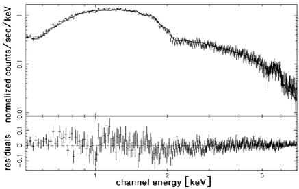
Figure 1: We show (upper panel) the observed X-ray spectrum of A1689 from the combined observations ID 540, 1663 and 5004 in the $0.5-7$ keV band, reduced from a $3^{\prime}$ aperture. The fit (solid curve) is to a MEKAL model with Galactic absorption fixed at the observed value. We also show (lower panel) the residuals of the fit.

3.1 Heavy element abundances

Before assessing the observed temperature profile it is important to determine the gas metal abundance. In principle, these two quantities may be decoupled with high quality data; however, the limited spectral resolution and signal-to-noise ratio means that the abundance is generally hard to constrain independently with radius, and one must adopt a mean value for the cluster. Vikhlinin et al. (2005) took advantage of the superior spatial resolution of Chandra to show that for a sample of nearby relaxed clusters there is a metallicity gradient such that the abundance increases toward the center. However, the high roughly solar abundance level is actually in a region coinciding with the central galaxy. On the theoretical side, Arieli, Rephaeli & Norman (in preparation) have performed a high resolution hydrodynamical simulation which uses a new approach to incorporate feedback from galaxies on the intracluster gas, and have shown that including physical processes such as galactic winds and gas stripping yields a flat metallicity profile out to large radii ($\sim 600$ h${}_{0.7}^{-1}$ kpc). Based on XMM data, AM04 showed that there is no abundance gradient in A1689. Our deduced abundance gradient is shown in figure 2. There is a systematic trend towards a higher value of $A$ in the Chandra data (in accord with the result of XW02) than the corresponding XMM value, but this difference is not very significant from a statistical point of view, since most of the data points agree within the $1\sigma$ range. The two sets of observations have the same exposure time, so the XMM data are more precise (due to the larger effective area). Our analysis indicates a fairly constant abundance over the region probed. In what follows we use the mean value of $0.4$ solar for the central $3^{\prime}$ region.

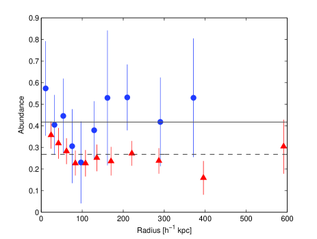
Figure 2: The abundance profile as derived from the spectral deprojection fitting. We compare our Chandra analysis (circles), which gives a mean value of $0.42$ (horizontal solid line), to the XMM analysis of AM04 (triangles) which gave a mean value of $0.27$ (horizontal dashed line).

3.2 Surface brightness and temperature analysis

An HST/ACS image of A1689 overlaid on the X-ray map is shown in figure 3; the cD galaxy lies at the X-ray centroid.

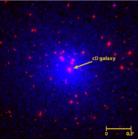
Figure 3: HST/ACS image of A1689 overlaid on smoothed color rendering of the X-ray emission (obs. ID 5004). The cD galaxy is seen to coincide with the X-ray centroid. The scale in the image is $0.5^{\prime}\simeq 65$ h^-1 kpc.

The symmetry of the surface brightness distribution allowed us to construct an azimuthally averaged profile in radial bins. We determined an azimuthally averaged flux $F$ in each radial bin by fitting the model to the data in each annulus and extracting the flux, from which the surface brightness $S$ was found by dividing by the angular area of the bin. The error in $S$ was calculated from that in the normalization parameter of the fitted model. Note that our profile of the surface brightness is $\sim 4$ times higher than that obtained by XW02 (see their Figure 6), but is consistent with that obtained by Mohr, Mathiesen & Evrard (1999, hereafter MME99; see their Figure 13).

The full extraction region consists of 50 annuli, each of width 4^″, plus nine annuli with varying widths (to keep adequate S/N) beyond 200^″, all centered on the cluster X-ray center (section 2.1). The maximum aperture of the data reduction region was limited by the outer edges of CCDs in practically all three observations. We removed the innermost ring because it corresponds to the inner region of the cD galaxy (see also Vikhlinin et al. (2005); e.g., the abundance in it was measured to be $0.9$, contrary to our assumption of a constant abundance in each annulus.

The reduction of the temperature profile was done in a similar way, but with a smaller number of annuli due to the lower signal-to-noise ratio.

4 Derivation of the Gas and Mass Profiles

4.1 Methodology

In this section we present our procedure for studying the structure of the cluster using all the available data sets in combination. Since we have both lensing and surface brightness profiles, we do not need to assume any particular parametrization or fitting formula, such as the commonly adopted NFW mass profile or the $\beta$ model for the gas density profile. We employ a model-independent approach that is limited only by the resolution and accuracy of the data. As mentioned in the introduction, the cluster has only a small ellipticity, so the assumption of spherical symmetry is reasonable. This basic assumption allows us to reconstruct three-dimensional profiles from the observed two-dimensional ones. The lensing data yields in this way the density profile of the total mass (dark matter plus gas), while the surface brightness profile depends on a combination of the gas density and temperature. Thus, with one additional relation, we can reconstruct the full gas and dark matter density profiles. We derive this additional relation by assuming hydrostatic equilibrium, consistent with the indications discussed in section 1 that A1689 is well relaxed. Hydrostatic equilibrium involves the gravitational force and thus inserts a dependence on the total mass profile that couples the constraints from lensing and from the X-ray data.

We determined the best-fit values of our free parameters by fitting the lensing and X-ray surface brightness data simultaneously. It is important to note that we did not include the temperature profile data for reasons that are explained later in this section. In our model-independent approach, our free parameters are the values of the 3D profile of the total mass density and the gas mass density at several fixed radii (logarithmically spaced). The radial ranges of the free parameters of the total mass density and the gas density were determined by the range of the lensing data and the X-ray surface brightness data, respectively. Within these ranges the density values were linearly interpolated (in log-log) in-between the fixed radii. Beyond the last data point, each profile (i.e., of the total mass density and the gas density) was extrapolated. The total mass density profile was extrapolated as $\rho(r)\propto r^{-3}$, in accordance with the asymptotic behavior of the NFW profile and also close to our best-fit core plus power-law model (section 5.2 below). The gas density was also extrapolated as $\rho(r)\propto r^{-3}$, in order to have a constant $f_{\rm gas}$ at large radii; this is also consistent with the previously deduced index of 2.9 (Xue & Wu 2000).

In spherical symmetry, the hydrostatic equilibrium equation for an ideal gas can be integrated from a given three-dimensional radius $r$ out to infinity (or some maximum, cutoff radius). This yields the relation

$$\left[\rho_{\rm gas}(r)T(r)\right]\Big{|}^{r}_{\infty}=\int^{\infty}_{r}\frac{GM_{\rm tot}(\leq r^{\prime})\mu m_{p}\rho_{\rm gas}(r^{\prime})}{kr^{\prime 2}}\,dr^{\prime}\ ,$$ (1)

where $\rho_{\rm gas}$ is the gas mass density, $T$ is the gas temperature, $M_{\rm tot}(\leq r)$ is the total mass within $r$, $\mu$ is the mean molecular weight, and $m_{\rm p}$ is the proton mass. Of course, $\mu$ depends on the abundances; the typical metal abundance is $\approx\frac{1}{3}$ (which is expected when ejecta are from Type Ia supernovae winds (Silk 2003)). In A1689, $A=0.2-0.49$ was found by XW02.

For given model parameters, the comparison to the lensing data was performed by first projecting the 3D profile of the total mass density using Abel integration

$$\kappa(R)=\frac{2}{\Sigma_{crit}}\int^{\infty}_{R}\frac{\rho_{\rm tot}(r)rdr}{\sqrt{r^{2}-R^{2}}}\ ,$$ (2)

where $\rho_{\rm tot}(r)$ is the three dimensional total mass density and $\Sigma_{crit}=\frac{c^{2}}{4\pi G}\frac{D_{\rm os}}{D_{\rm ol}D_{\rm ls}}$ is the critical density for lensing, written in terms of angular diameter distances $D_{\rm os}$ (observer–source), $D_{\rm ol}$ (observer–lens), and $D_{\rm ls}$ (lens–source). Simultaneously, we calculated the mass profile using

$$M_{\rm tot}(\leq r)=4\pi\int^{r}_{0}\rho_{\rm tot}(r^{\prime})r^{\prime 2}dr^{\prime}\ .$$ (3)

We then used the mass profile and the gas density profile in the hydrostatic equilibrium equation (1), obtaining the temperature profile. The temperature and gas density profiles were then used (with the assumed abundances) to determine the emissivity:

$$\varepsilon(r)=n_{e}(r)n_{H}(r)\Lambda(T(r))\ ,$$ (4)

where $\Lambda(T)$ is the cooling function, which was obtained by considering all the relevant physical processes in the $9\cdot 10^{5}-3\cdot 10^{8}$ K range. The cooling function was calculated by MEKAL (consistent with our fitting of the observed spectra in section 2.1). We use the usual definitions, $n=\rho_{\rm gas}/(\mu m_{p})$, $n_{e}=\rho_{\rm gas}/(\mu_{e}m_{p})$, and $n_{H}=\rho_{\rm gas}/(\mu_{H}m_{p})$, which for $A=0.4$ solar yield $\mu=0.55$, $\mu_{e}=1.05$, and $\mu_{H}=1.30$.

Having thus obtained the emissivity, we re-projected it using the Abel integral and obtained the X-ray surface brightness

$$S(R)=1.191\cdot 10^{-12}\frac{\pi}{(1+z)^{4}}\int^{\infty}_{R}\frac{\varepsilon(r)rdr}{\sqrt{r^{2}-R^{2}}}\ ,$$ (5)

where $\varepsilon$ is the emissivity in erg s^-1 cm^-3, $S$ is the X-ray surface brightness in erg s^-1 cm^-2 arcsec^-2, and we converted the units from erg s^-1 cm^-2 to erg s^-1 cm^-2 arcsec^-2 by multiplying by $\frac{D_{A}^{2}}{4\pi D_{L}^{2}}$, using $D_{L}/D_{A}=(1+z)^{2}$ (where $D_{L}$ and $D_{A}$ are the angular diameter and luminosity distance, respectively), and upon conversion of radians^-2 to arcsec^-2. The mean surface brightness was calculated in each annulus-shaped bin within the surface brightness data. The mean surface brightness $S_{\rm bin}$ in a bin with inner and outer radii $R_{\rm in}$ and $R_{\rm out}$, respectively, is

$$S_{\rm bin}=\frac{2}{(R_{out}^{2}-R_{in}^{2})}\int^{R_{out}}_{R_{in}}RS(R)dR\ .$$ (6)

Finally, we compared this to the surface brightness data.

Having calculated the observed quantities for each possible set of model parameters, we then compared to the data using a $\chi^{2}$ measure. The total $\chi^{2}$ is the sum of two terms, one from the lensing data and one from the X-ray surface brightness data:

$$\chi^{2}=\chi^{2}_{\kappa}+\chi^{2}_{S}\ ,$$ (7)

where

$$\chi^{2}_{\kappa}=\sum_{i=1}^{N_{\kappa}}\left[\frac{\kappa(R_{i})-\kappa_{data}(R_{i})}{\Delta\kappa_{data}(R_{i})}\right]^{2}$$ (8)

and

$$\chi^{2}_{S}=\sum_{j=1}^{N_{S}}\left[\frac{S_{\rm bin}(R_{j})-S_{data}(R_{j})}{\Delta S_{data}(R_{j})}\right]^{2}\ .$$ (9)

Here $\chi_{\kappa}^{2}$ is the $\chi^{2}$ of the lensing data, obtained by comparing the model $\kappa$ of equation (2) with the $N_{\kappa}$ data points $\kappa_{data}$ and their errors $\Delta\kappa_{data}$; similarly, $\chi_{S}^{2}$ is the $\chi^{2}$ of the X-ray surface brightness data, obtained by comparing the model $S$ of equation (6) with the $N_{S}$ data points $S_{data}$ and their errors $\Delta S_{data}$. The best-fit values of the parameters, which are the 3D profile of the total mass density and the 3D gas density profile, were obtained by minimizing the total $\chi^{2}$. From these two profiles we then derived the three dimensional temperature profile using equations (1) and (3). In order to perform an independent consistency check with the two-dimensional temperature data (which were not used in the analysis), we projected the 3D temperature, weighting it by the emissivity for comparison with the observed temperatures:

$$T_{\rm 2D}(R)=\frac{\int^{\infty}_{R}T(r)\,\varepsilon(r)\,\frac{r}{\sqrt{r^{2}-R^{2}}}\,dr}{\int^{\infty}_{R}\varepsilon(r)\,\frac{r}{\sqrt{r^{2}-R^{2}}}\,dr}\ .$$ (10)

Weighting by the emission measure EM (which is proportional to $\rho_{\rm gas}^{2}$) gave similar results.

The EM weighted temperature ($T_{EM}$) and the emissivity weighted temperature ($T_{E}$) may not precisely reflect the actual spectral properties of the observed source. Vikhlinin (2005) states that the ”spectroscopic” temperature is generally lower than either of these temperatures, although his suggested correction formula for the effective spectroscopic temperature of a multi-component thermal plasma yielded similar values to $T_{EM}$ and $T_{E}$. Mathiesen & Evrard (2001) claimed that the observed spectroscopic temperature may be biased low due to the excess of soft X-ray emission from the small clumps of cool gas that continuously merge into the intracluster medium. Furthermore, Mazzotta et al. (2004) showed that from a purely analytical point of view the spectrum of a multi-temperature thermal model cannot be accurately reproduced by any single-temperature thermal model. It has also been found in simulations that the spectral temperature is in general smaller than $T_{E}$ by a factor of $0.7-0.8$ (Rasia et al. 2005). We note that total mass estimates obtained based solely on X-ray data together with the assumption of hydrostatic equilibrium depend strongly on the temperature. In our analysis, however, we do not use the temperature data for the fit but only for a consistency check. Therefore, our values for the total mass density are determined mainly by the lensing data.

Our analysis focuses on the free-parameter method that does not assume a particular shape for the profile. In addition, we used our analysis method to test the viability of either an NFW profile or a cored profile.

4.2 The entropy profile

It is interesting to evaluate the entropy and the adiabatic index profiles in order to probe the processes that govern the thermal state of intracluster gas. For a monoatomic ideal gas $s=\frac{3}{2}k\ln K+s_{0}$, where $s=\frac{S}{N}$ is the entropy per particle and $K\equiv T\,n^{-2/3}$. In this case $K$ is a combination of $n$ and $T$ that is invariant under adiabatic processes in the gas. More generally, $T\propto n^{\Gamma-1}$ under adiabatic changes, where $\Gamma$ is the adiabatic index. In this paper we refer to $K$ as the “entropy”.

The gas at $\sim 0.1R_{\rm vir}$ lies outside of the cooling region, and is still sufficiently close to the cluster center where shock heating is minimized (Lloyd-Davis, Ponman, & Cannon 2000). Thus at this radius, it is less sensitive to specific models and assumptions. In the outer regions, $r\gtrsim 0.1R_{\rm vir}$, the entropy is entirely due to gravitational processes, and the entropy profile is expected to be a featureless power law approaching $K\propto r^{1.1}$ (Tozzi & Norman 2001; Voit, Kay, & Bryan 2005). In the inner region the gas entropy profile is flattened (for ASCA and ROSAT data, see Lloyd-Davis, Ponman, & Cannon 2000; Ponman, Sanderson,& Finoguenov 2003; for various cosmological simulations see Voit, Kay, & Bryan 2005; for a theoretical analysis of joint X-ray and SZ observations, see Cavaliere, Lapi, & Rephaeli 2005) .

4.3 The effect of the cD galaxy

A massive cD galaxy dominates the inner region of A1689. Thus, it is important to check the effect of the cD galaxy on the cluster, and especially on the 2D temperature observed in the central region. Its mass profile can be analytically expressed as follows. The mass profile is $M_{\rm cD}=M_{\rm stars}+M_{\rm DM}$, where the gas mass is neglected since it is dominated by the stellar mass at small radii and by the DM mass at large radii. We assume an NFW profile for the dark matter, and express the stellar mass profile as $M_{\rm stars}=M_{\rm stars,0}\cdot\frac{r^{2}}{(r+a)^{2}}$, where $M_{\rm stars,0}$ is the mass of the stars in the cD galaxy and $a$ is a characteristic length-scale (Hernquist 1990). Typical values for the effective radius, $R_{e}$, with $a=R_{e}/1.82$, are $R_{e}\approx 3-5$ h^-1 kpc. E.g., Jannuzi, Yanny, & Impey (1997) found an average $R_{e}=4.6$ h^-1 kpc for five elliptic galaxies; Brown & Bregman (2001) found an average $R_{e}=3.2$ h^-1 kpc for four elliptical galaxies (but see Arnalte Mur, Ellis, & Colless (2006) who found $R_{e}=24.7$ h^-1 kpc). Typical values for the characteristic radius of the NFW profile of the DM (see also section 5.2 below) are $5-25$ h^-1 kpc (Romanowsky et al. 2003).

X-ray emission from the cD galaxy may be produced by the stars and stellar remnants, or by the hot gas. For the stellar component, the spectrum (dominated by X-ray binaries) is expected to be hard like that of the cluster ($T_{X}\sim 10$ keV) and have a minor effect on the measured 2D temperature, so we did not include it in our model. We considered the gas emission, which should give a soft spectrum ($T_{X}\sim 1$ keV) (Brown & Bregman 2001). We adopted a double beta model for the gas density profile, as Matsushita et al. (2002) fitted to M87, where we redid the fit to the M87 data, allowing the parameters to vary freely except that we fixed the $\beta$ of the extended component to be $0.47$ (based on data from the ROSAT all sky survey: Bohringer et al. 1994). For a given gas mass density and total mass profile of the cD, we derived the temperature using equation (1). From the gas density and the temperature we obtained the emissivity using the MEKAL code, assuming a solar metal abundance.

5 Results

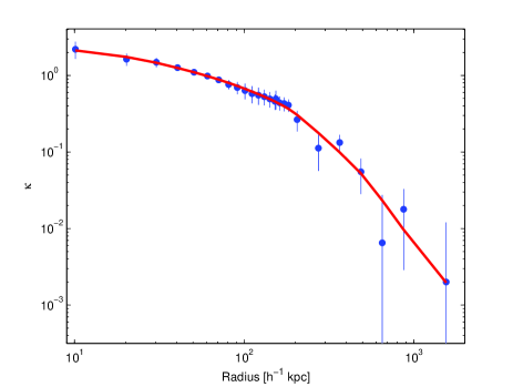
Figure 14: Our fit to the lensing data. The $\kappa$ profile obtained by our model-independent method (solid curve) is compared to the measured profile (points with error bars), where $\kappa$ is the 2D surface density in units of the critical density for lensing.

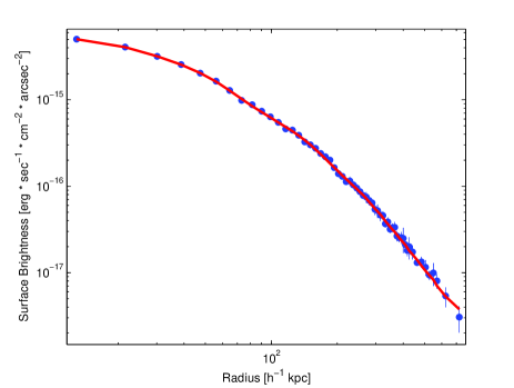
Figure 15: Our fit to the surface brightness data. The X-ray surface brightness profile obtained by the model-independent method (solid curve) is compared to the measured profile (points with error bars).

In this section we present the results of our model-independent analysis of the lensing and X-ray data. The numbers of data points used in the analysis were $N_{\kappa}=26$ and $N_{s}=58$ for lensing and surface brightness, respectively. Accordingly, the ratio of the number of free parameters for the total mass to that for the gas mass profile was set to $i/j\approx 26/58$. As our standard case, we chose 6 free parameters for the total mass density and 14 free parameters for the gas mass density. These relatively small numbers of model points ensured fairly smooth profiles that effectively average over the noise in the data. The fit to the lensing and surface brightness data can be seen in fig. 14 and fig. 15, respectively. Both of the fits are very good, as expressed in the low reduced $\chi^{2}$, i.e., $\chi^{2}_{\rm r}\equiv\chi^{2}/$dof. The reduced $\chi^{2}$ of the fit to the data was 28.1/64. The contribution of each data set within the total, simultaneous fit to both, was $\chi^{2}_{r}({\rm lensing})=4.7/20$ and $\chi^{2}_{r}({\rm surface\;brightness})=23.5/44$. This shows that we achieved a good fit to both data sets, and thus did not need a larger number of model points. The low $\chi^{2}_{\rm r}$, especially in the lensing case, suggests errors that are either overestimated or significantly correlated among the various data points, producing smoother data than expected given the errors. For a consistency check, we repeated the fits with different numbers of parameters, namely $i=5,j=11$ and $i=4,j=9$. In figures 4 – 6 we show the profiles of the total mass density, the gas mass density, and the temperature for the three free parameters sets, ($i=5,j=11$), ($i=6,j=14$) and ($i=4,j=9$). The figures clearly show that our results are insensitive to the precise number of adopted free parameters. To assess the degree of correlation between values of the projected fit parameters we have calculated the correlation matrix for $i=4,j=9$, which is specified in table 8 in the Appendix.

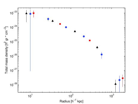
Figure 4: Results for the total mass density profile when different numbers of free parameters are used for the profiles of total mass ($i$) and gas ($j$). We consider $i=6$, $j=14$ (circles), $i=5$, $j=11$ (triangles), and $i=4$, $j=9$ (squares). All three cases had the same, fixed values for the smallest and largest radius; these sets of points have been offset for display purposes, the triangles to the left and the squares to the right.

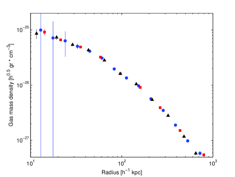
Figure 5: Results for the gas mass density profile when different numbers of free parameters are used. Sets of points are as in figure 4. The first and last points are offset as in figure 4.

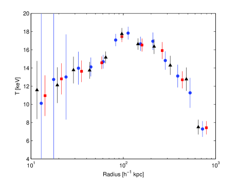
Figure 6: Results for the 3D temperature profile when different numbers of free parameters are used. Sets of points are as in figure 4. The first and last set of points are again offset as in figure 4.

We tested the effect of the form of extrapolation to large radii on the values obtained for the total mass density and the gas mass density. We checked the results for large changes in the extrapolation power-law index, i.e. $-2$ and $-4$ (compared to our standard assumption of $\rho\propto r^{-3}$). We used our standard number of free parameters, $6$ and $14$ for the total mass density and for the gas mass density, respectively. In each case the same extrapolation index was used for the total mass and the gas mass density in order to ensure a constant gas fraction at large radii. We expected a large change in the free parameter at the largest radius, which is the closest to the extrapolation. Using an extrapolation index $-2$ gave a value which is lower by $21\%$ and $11\%$ for the total mass density and gas mass density, respectively, at this last point. For an extrapolation index $-4$ there was $<1\%$ change in the total mass density value and $8\%$ in the gas mass density. In the gas mass density there was also a change in the innermost radius, $29\%$ and $36\%$ for an extrapolation index of $-2$ and $-4$, respectively; this change is not very significant due to the large errors at this radius. Taking a smaller number of free parameters lowers the errors of the gas mass density at the smaller radius and as a consequence also weakens the dependence on the extrapolation index. Thus, our results in general are not strongly dependent on the extrapolation index.

5.1 Total mass density

The values of our six free parameters of the total mass density and the deduced 3D mass are shown in table (3). As mentioned above the X-ray temperature data were not used. The surface density data were used, but their effect on the total mass profile is limited since $\rho_{\rm gas}$ appears on both sides of equation (1). Thus, the lensing data basically determined the derived 3D total mass density and the 3D mass profiles.

Table 3: Values of 3D mass density; errors are 1-$\sigma$ confidence.

$r$ [h-1 kpc]	$\rho_{\rm total}$ [$10^{-25}$ h2 gr/cm3]	$M_{\rm total}$ [$10^{12}$ h-1 $M_{\sun}$]
10.1	$90_{-90}^{+91}$	$0.91\pm 0.68$
27.7	$39\pm 11$	$7.3\pm 2.5$
75.9	$10.5\pm 1$	$48.3\pm 3.9$
208	$2.4\pm 0.4$	$252\pm 15$
568	$0.13\pm 0.07$	$679\pm 82$
1554	$0.0022_{-0.0022}^{+0.0049}$	$956\pm 180$

We also compared the total mass density profile obtained by the model-independent method to the that obtained by fitting particular models. We tested the NFW profile,

$$\rho=\frac{\rho_{0}}{\left(r/r_{s}\right)\left(1+r/r_{s}\right)^{2}}\ ,$$ (11)

and a core model,

$$\rho=\frac{\rho_{0}}{\left(1+(r/r_{s})^{2}\right)^{n}}\ ,$$ (12)

where $r_{s}$ is a scale radius. In the NFW profile $\rho_{0}$ and $r_{s}$ were free parameters, and in the core profile $\rho_{0}$, $r_{s}$, and $n$ were free parameters.

Table 4: The values of the parameters of the two total mass density models, NFW and core. The errors are 1-$\sigma$ confidence.

Parameter	NFW	core
$\rho_{0}$ [$10^{-25}$ h2 gr/cm3]	$9.6\pm 1.8$	$24.4\pm 4.5$
$r_{s}$ [h-1 kpc]	$175\pm 18$	$91\pm 17$
n	-	$1.43\pm 0.12$
$\chi^{2}/dof$	$15.3/(26-2)$	$13.3/(26-3)$

We chose these two profiles since they are frequently used and are significantly different both at small and at large radii. For simplicity, we fitted the two profiles only to the lensing data.

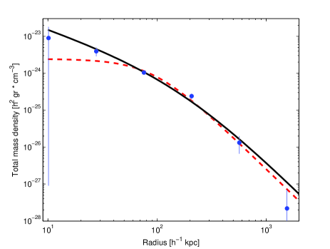
Figure 7: A comparison between the mass profile derived by the model-independent method to that using particular models. We compare the values obtained by our model-free analysis (points with error bars) to the results of assuming an NFW profile (solid curve) or a core plus power-law profile (dashed curve).

A comparison of the profiles to the six values we obtained in our main analysis (figure 7 and table 4) yields a fairly close agreement and implies that neither of the profiles is strongly excluded. Still, the measured profile as sampled by the six points is steeper at large radii than both models, in agreement with Broadhurst et al. (2005b). The core profile is too shallow at small radii and thus seems not to be a good fit to our deduced values of the mass density in this region.

The NFW fit gave a concentration parameter $C_{N}=12.2^{+0.9}_{-1}$, where $C_{N}=r_{\rm vir}/r_{s}$ in terms of the virial radius $r_{\rm vir}$ and the characteristic radius $r_{s}$ of the NFW profile. This is close to the value obtained by Broadhurst et al. (2005b), $C_{N}=13.7^{+1.4}_{-1.1}$, which was based only on a fit to the strong and weak lensing information. We also obtained from the NFW fit two characteristic radii for the cluster: $r_{200}$, the radius inside which the average density is $200$ times the critical density, and $r_{\rm vir}$, defined with a relative density of $116$, which is the density expected theoretically at $z=0.183$ in the $\Lambda$CDM model. The fit yielded $r_{200}=1.71$ h^-1 Mpc and $r_{vir}=2.14$ h^-1 Mpc.

In figure 8 we plot our derived 3D total mass profile from eq. (3) and the one derived in AM04 from XMM data. They used an NFW profile based on data out to $693$ h^-1 kpc. The two profiles agree at the small radii but disagree at larger radii. Our highest-radius point agrees with their profile, but at this radius we had to extrapolate the AM04 3D mass profile beyond their data range.

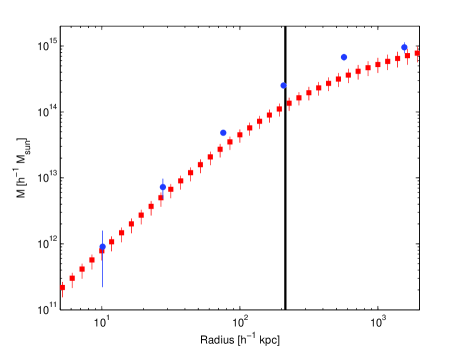
Figure 8: The derived 3D total mass profile. We compare our derived profile (dots) to the one derived by AM04 (squares). They used an NFW profile based on data out to $693$ h^-1 kpc. Both profiles are shown with 1-$\sigma$ errors. The vertical dotted line is at 0.1 $r_{\rm vir}$.

5.2 2D mass profile

The deduced 2D mass profile $M_{2D}(R)=2\pi\Sigma_{crit}\int_{0}^{R}\kappa(R^{\prime})R^{\prime}dR^{\prime}$, is compared with previous results in Figure 9. These include results from strong lensing (Tyson & Fischer 1995), the lensing magnification measured by the distortion of the background galaxy luminosity function (Dye et al. 2001), the lensing magnification measured by the deficit of red background galaxies (Taylor et al. 1998), the projected best-fit NFW model from X-ray data (AM04 via XMM), and the best-fit NFW model from weak gravitational shear analysis (Clowe & Schneider 2001; King et al. 2002). The latter analysis, although it is a weak lensing analysis, is the closest to the profile derived from X-ray data, but it appears to have underestimated the distortion signal derived in the other lensing analyses. This is probably caused by confusion between the cluster galaxies and the foreground or background galaxies. Thus, the X-ray analysis of AM04 (based on the X-ray temperature) gives a substantially lower 2D mass than the more reliable lensing analyses. This foreshadows the discrepancy that we find with the measured temperature (see section 5.5 below).

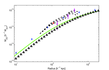
Figure 9: The derived 2D mass profile (6 diamonds) is compared to the gravitational lensing results from strong lensing (square, Tyson & Fischer 1995), distortion of background galaxy luminosity function (3 circles, Dye et al. 2001), deficit in number counts of red background galaxies (dashed curves, Taylor et al. 1998), projected best-fit NFW model from weak gravitational shear (triangles, King et al. 2002), and projected best-fit NFW model from X-ray data (solid curve, AM04) .

5.3 Gas density profile

The values of the derived gas mass density are shown in table 5. We compared our gas density profile to the one obtained by MME99. They fitted a single $\beta$ model to the surface brightness profile; in clusters where they suspected the presence of cooling flows the fit was to a double $\beta$ model (though with the same $\beta$ in both elements). They used two types of clues for the presence of cooling flows. First, when fitting a single $\beta$ model the surface brightness data points must be higher than the fitted curve in the inner region. Second, the cluster must appear relaxed, i.e., lacking obvious asphericity or substructure that would indicate a recent merger. Judging by their successful fit to a single $\beta$ model, they concluded that A1689 is not likely to have a cooling flow. Their fit is thus based on an assumed isothermal profile, and $0.3$ solar abundance. Figure 10 shows excellent agreement between our obtained gas density profile and the one obtained by MME99.

Table 5: Deduced values of the 3D gas mass density, and derived temperatures using the gas and total mass profiles together with the hydrostatic equilibrium equation. The errors are 1-$\sigma$ confidence.

$r$ [h-1 kpc]	$\rho_{\rm gas}$ [$10^{-26}$ h0.5 gr/cm3]	$T_{3D}$ [keV]
12.9	$9.9_{-9.9}^{+30.3}$	$10.1_{-10.1}^{+30.5}$
17.6	$7.2_{-7.2}^{+10.7}$	$12.7_{-12.7}^{+15.5}$
24.0	$6.4\pm 3.1$	$13.0\pm 4.7$
32.7	$5.06\pm 0.55$	$14.0\pm 1.8$
44.5	$4.12\pm 0.18$	$14.1\pm 1.0$
60.7	$3.09\pm 0.11$	$14.7\pm 0.75$
82.7	$1.96\pm 0.055$	$17.1\pm 0.7$
113	$1.35\pm 0.033$	$17.8\pm 0.7$
154	$0.97\pm 0.023$	$16.65\pm 0.78$
209	$0.567\pm 0.015$	$16.94\pm 0.96$
285	$0.35\pm 0.012$	$14.8\pm 1.0$
388	$0.19\pm 0.0079$	$13.1\pm 1.3$
529	$0.0982\pm 0.00067$	$11.3\pm 1.7$
721	$0.0586\pm 0.00057$	$7.29\pm 0.87$

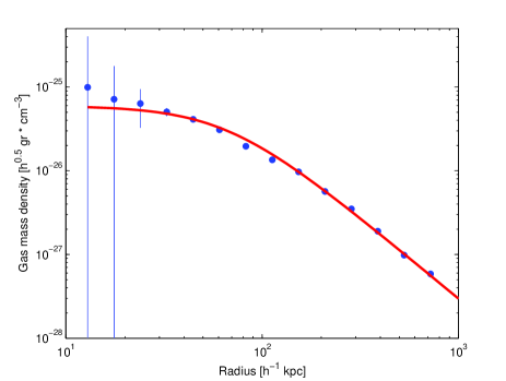
Figure 10: Our derived gas mass density profile (points with error bars) compared to the profile derived by MME99 (solid curve).

Table 6: Deduced values of the 3D gas mass at various radii. The errors are 1-$\sigma$ confidence.

$r$ [h-1 kpc]	$M_{\rm gas}$ [$10^{11}$ h-5/2 $M_{\sun}$]
12.9	$0.20_{-0.20}^{+0.60}$
17.6	$0.37_{-0.37}^{+0.70}$
24	$0.71\pm 0.57$
32.7	$1.44\pm 0.68$
44.5	$2.93\pm 0.64$
60.7	$5.85\pm 0.66$
82.7	$10.93\pm 0.65$
113	$19.46\pm 0.66$
154	$34.63\pm 0.67$
209	$59.3\pm 0.74$
285	$96.83\pm 0.88$
388	$151.5\pm 1.3$
529	$224.8\pm 2.5$
721	$328.4\pm 3.7$

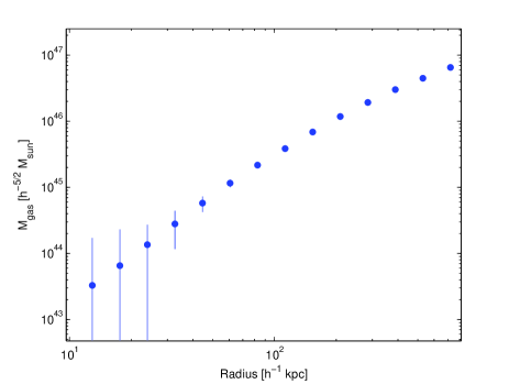
Figure 11: The gas mass profile derived from the best-fit gas density profile. All the values have error bars but some are too small to distinguish. These values are also listed in table (6).

5.4 Gas mass fraction

Having derived the total and gas mass densities, the gas fraction, $f_{\rm gas}=M_{\rm gas}/M_{\rm total}$, can then be determined upon integration. We can compare our value, $f_{\rm gas}(r=0.25r_{200})=0.0326\pm 0.0023$ h^-3/2, to Sanderson et al. (2003). They obtained for the $8-17$ keV range (see their figure 6) $f_{\rm gas}(r\cong 0.25r_{200})=0.041$ h^-3/2. Our value of $r_{200}$ is slightly different since it was derived from the NFW fit to the lensing data, whereas their value was deduced from the X-ray data. They obtained $r_{200}=2955$ h${}_{0.7}^{-1}=2068.5$ h^-1 kpc, and if we scale our result by their $r_{200}$ we get $f_{\rm gas}(r=0.25r_{200})=0.0359\pm 0.0024$ h^-3/2. This value is still somewhat lower than their $8-17$ keV value, but in good agreement if we look at the scatter of the gas fraction in their figure 4. In their figure 4 they plotted the values of the gas fraction of different clusters at $r=0.3r_{200}$ as a function of the cluster temperature. The gas fraction of hot clusters ranges from $\sim 0.035$ h^-3/2 to $\sim 0.06$ h^-3/2, with some $\sim 40\%$ uncertainty. AM04 found for A1689 $f_{\rm gas}(r=r_{2500})=0.044\pm 0.0049$ h^-3/2, which is in agreement with our value of $f_{\rm gas}(r=r_{2500})=0.0385\pm 0.0026$ h^-3/2. MME99 found for an ensemble of clusters with $T>5$ keV a $f_{\rm gas}(r=r_{500})=0.075$ h^-3/2, close to and slightly lower than the value in Sanderson et al. (2003), just as our gas fraction at $r=0.25r_{200}$ was a little lower than the value derived by Sanderson et al. (2003) at that radius.

Markevitch et al. (1999) examined two relaxed clusters, A2199 and A496, which are cooler than A1689 and have temperatures $\sim 4-5$ keV. They found $f_{\rm gas}(r=0.5\;h^{-1}\;{\rm Mpc})=0.0569\pm 0.0049$ h^-3/2 and $f_{\rm gas}(r=0.5\;h^{-1}\;{\rm Mpc})=0.0559\pm 0.006$ h^-3/2 for A2199 and A496, respectively. These values are slightly higher than in other papers. They claimed that their values are consistent with others including MME99, who found that $\langle f_{\rm gas}\rangle=0.0566$ h^-3/2 for clusters with $T<5$ keV. However, note that the Markevitch et al. values are at $r_{1000}$ while the MME99 values are at $r_{500}$.

The gas mass fraction was also determined from SZ measurements with BIMA and OVRO (Grego et al. 2001). The latter authors measured $f_{\rm gas}(r=65")$ and used a scaling relation in order to obtain $f_{\rm gas}(r=r_{500})$. They found for a sample of 18 clusters (assuming $\Omega_{m}=0.3$, $\Omega_{\Lambda}=0.7$) $f_{\rm gas}=0.081^{+0.009}_{-0.011}$ h^-1. These values are higher than obtained by X-ray measurements. For A1689, Grego et al. (2001) obtained $f_{\rm gas}(r=r_{500})=0.098^{+0.029}_{-0.033}$ h^-1, or more directly $f_{\rm gas}(r=65")=0.068^{+0.02}_{-0.023}$ $h^{-1}$. Our results yield $f_{\rm gas}(r=r_{500})=0.0482$ h^-3/2 and $f_{\rm gas}(r=65"=140\;h^{-1}\;{\rm kpc})=0.0222\pm 0.0009$ h^-3/2, much lower than in their paper. Some systematic discrepancy in the gas fraction from X-ray and SZ measurements is expected (Hallman et al. 2007). The difference can be due to the fact that $M_{\rm gas}({\rm SZ})\propto T^{-1}$ (where $T$ is the gas temperature as deduced from spectral X-ray measurements; Grego et al. 2001), since (the thermal component of) the SZ effect depends on the product of gas density and temperature. Thus, an underestimation of the temperature (see section 5.5) results in an $M_{\rm gas}({\rm SZ})$ that is higher than $M_{\rm gas}(\mbox{X})$, making $f_{\rm gas}({\rm SZ})$ higher than $f_{\rm gas}(\mbox{X})$. Expressing the difference in terms of the gas mass, Grego et al. (2001) obtained $M_{\rm gas}(r=65")=4.6_{-1.1}^{+0.8}\cdot 10^{12}$ h^-2 $M_{\odot}$ and we $M_{\rm gas}(r=65")=2.9\cdot 10^{12}$ h^-1 $M_{\odot}$. The ratio between the gas fraction derived by X-rays and the one derived by SZ also depends on clumpiness, where we define the clumping parameter as $C\equiv\langle n_{e}^{2}\rangle^{1/2}/\langle n_{e}\rangle$. The gas mass measured via X-ray is $M_{\rm gas}(\mbox{X})\propto C^{-1}$, i.e., the actual gas mass is lower than that apparently observed if the cluster is clumpy but this is not corrected for. The gas mass measured via SZ is not proportional to the clumping. Thus, correcting for clumping would further decrease $M_{\rm gas}(\mbox{X})/M_{\rm gas}({\rm SZ})$ by a factor of $\sim C$. This may indicate that the level of clumping in this cluster is low.

Finally, we also compared our results for the gas fraction to the simple theoretical models. In figure 12 we show the $f_{\rm gas}$ obtained by the parametrized models, NFW (solid curve) or core (dashed curve) for the total mass density and (in both cases) a double $\beta$ model for the gas mass density, compared to the profile obtained from our model-free method (points with error bars). In general the models are not far from our reconstructed values. At very large radii, extrapolated beyond the data points, the gas fraction derived by the models would diverge from the real, supposedly constant value at large radii, since $\rho_{\rm gas}\propto r^{~{}-2.2}$ and $\rho_{DM/total}\propto r^{-3}$. Instead, in our model-independent method the extrapolation of the gas density is $\rho_{\rm gas}\propto r^{-3}$, in order to give an asymptotic $f_{\rm gas}=$const at large radii. At radii of $\sim 200-500$ h^-1 kpc the $f_{\rm gas}$ obtained by the model-independent method tends to be slightly lower than the one obtained by the parametrized models. At small radii the NFW model fits better than the core model, though the core gives a better overall fit to the lensing data (see table 4).

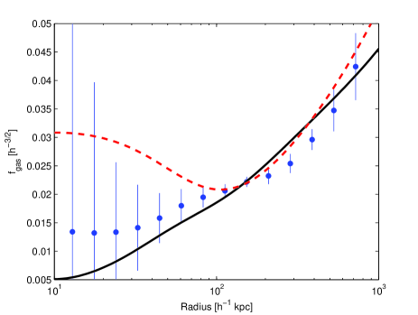
Figure 12: A comparison between the $f_{\rm gas}$ profile derived by our model-independent method (points with error bars) to the profile derived using parametrized models. We consider two simple models, NFW (solid curve) and a core profile (dashed curve) for the total mass, in each case with a double beta profile for the gas mass.

5.5 2D temperature profile

In figure 13 we compare the 2D temperature obtained by our model-free method to the measured 2D temperature. The measured 2D temperature is substantially lower. It has been found in numerical simulations that the spectroscopic temperature is typically lower than the one determined by hydrostatic equilibrium by a factor of $0.7-0.8$ (Rasia et al. 2005). Thus we also show in the figure the measured 2D temperature divided by 0.7 (upper solid curve). This factor explains most of the discrepancy in A1689. Kawahara et al. (2006) used cosmological hydrodynamical simulations to explain this discrepancy. They found that local inhomogeneities in the gas are largely responsible.

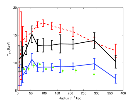
Figure 13: A comparison between the 2D temperature profile obtained from our model-independent method (dashed curve) to the profile measured from the X-ray spectrum (lower solid curve). Also shown are the measured temperature divided by 0.7 (upper solid curve) and the measured 2D temperature profile from AM04 (circles with error bars).

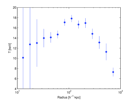
Figure 16: The 3D temperature profile as reconstructed by our model-independent method.

5.6 The entropy and polytropic index

Previous theoretical work has shown that the entropy profiles of non-radiative clusters approximately follow a power law with $K(r)\propto r^{1.1}$ (Tozzi & Norman 2001; Borgani et al. 2002; Voit et al. 2003). More recent detailed hydrodynamical simulations by Voit, Kay & Bryan (2005) confirmed the power law behavior of the entropy at $r>0.1r_{\rm vir}$. They also determined the normalization $N$, where $K(r)/K_{200}=N(r/r_{200})^{1.1}$, which was found to be $1.32\pm 0.03$ and $1.41\pm 0.03$ for SPH and AMR simulations, respectively. In the central region of the cluster, $<0.1r_{\rm vir}$, there are some claims for the existence of an entropy ”floor”, i.e., a limiting constant value. Voit et al. (2003) showed theoretically how an entropy floor can be attained; Voit, Kay & Bryan (2005) used simulations to find the level of this entropy floor. They found an entropy floor using an AMR code, but the value obtained with an SPH code was substantially lower (if at all present).

Observational comparisons of the entropy of clusters at small and at large radii show a departure from the predicted self-similarity. In the inner regions of low-mass clusters there appears to be a ”floor” in entropy of $\sim 135$ keV cm², with a higher value for high-mass clusters (Lloyd-Davies, Ponman, & Cannon 2000). This may represent a ”preheated” minimum level which Kaiser (1991) speculated may be due to the effect of star formation in early galaxies which preheat the IGM through galactic winds. This idea is strengthened by the ubiquitous presence of gas outflows in observations of high-redshift galaxies (Franx et al. 1997, Frye & Broadhurst 1998, Frye, Broadhurst & Benitez 2002, Pettini et al. 2001). Thus it seems natural to link this entropy floor with the winds from galaxy formation.

In figure 17 we plot $K/K_{200}$, where $K_{200}$ is the entropy at $r=r_{200}$. We find $r_{200}=1.7$ h^-1 Mpc and $r_{200}\cong 0.8r_{\rm vir}$. The value of our derived entropy at $0.1r_{\rm vir}$ agrees well with the one found by Lloyd-Davis, Ponman, & Cannon (2000), who used ROSAT and ASCA data. They assumed spherical symmetry and hydrostatic equilibrium, and a single beta model for the gas density along with a linear function for the temperature. For the DM density they used an NFW profile. Our derived entropy at $0.1r_{\rm vir}$, $K(r=0.1r_{\rm vir})=786\pm 33$ h^-1/3 keV cm², also agrees well with Ponman, Sanderson, & Finoguenov (2003), who also used ROSAT and ASCA data, assumed spherical symmetry and hydrostatic equilibrium, a single beta model for the gas density, and a linear function or a polytrope for the temperature. We fitted a power law to our entropy profile at all radii where we obtained the gas mass density (which includes points at $r<0.1r_{\rm vir}$). This fitted power law, which is shown in figure 17, is $K(r)/K_{200}=(0.95\pm 0.05)(r/r_{200})^{0.82\pm 0.02}$.

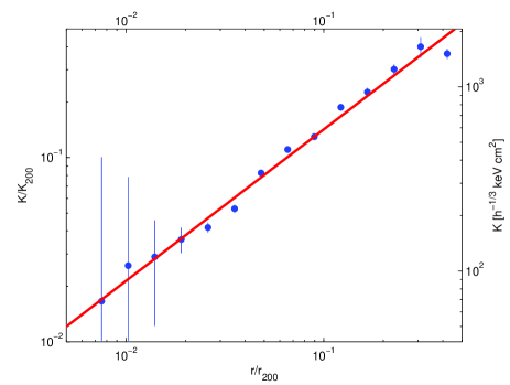
Figure 17: Our derived entropy profile (points with error bars) compared to the best-fit power law profile (solid curve).

Our X-ray data go up to $\sim 0.34r_{\rm vir}$, so obtaining a fit to the $(0.1-1)r_{\rm vir}$ range is not possible. In the available range $\sim(0.006-0.34)r_{\rm vir}$ the power law is a close fit, though the index is somewhat lower than the theoretical value of $1.1$. Excluding the entropy points at small radii, $r<0.1r_{\rm vir}$, would not substantially change the value of the power index, but then there are only four data points at $r>0.1r_{\rm vir}$. In the inner part ($r<0.1r_{vir}$) if the entropy is flattened then this occurs only at $r<0.02r_{vir}$. This is consistent with Tozzi & Norman (2001) who found that the flat entropy region in massive clusters ($M\sim 10^{15}$ $M_{\odot}$) occurs only at $r<0.01\;r_{200}$. Comparing our obtained values of the entropy at $r<0.1r_{\rm vir}$ to those in Voit, Kay & Bryan (2005), they are closer to the values obtained in the SPH simulations than in the AMR simulations. Our derived normalization $0.95\pm 0.05$ is somewhat lower than obtained by Voit, Kay, & Bryan (2005) in both types of simulations.

The deduced power law index is slightly lower than the value obtained from simulations (Tozzi & Norman 2001; Borgani et al. 2002; Voit et al. 2003; Voit, Kay, & Bryan 2005). The disagreement can be explained by the fact that we did not assume an NFW profile. Assuming an NFW profile gives $K(r)/K_{200}=(1.13\pm 0.39)(r/r_{200})^{1\pm 0.2}$. This is in good agreement with the ”expected” power law index of $1.1$. There is also a good agreement with the normalization obtained by simulations (Voit, Kay, & Bryan 2005). It has also been shown in simulations that as the amount of preheating increases, the power law index becomes flatter at radii beyond the flat inner region (Borgani et al. 2005).

In figure 18 we plot the adiabatic index. The solid curve is taken from Tozzi & Norman (2001). They used an NFW profile for the DM and assumed no cooling. They also assumed an external, initial adiabat for the entropy. Our derived adiabatic index profile is in reasonable agreement with the profile derived by Tozzi & Norman (2001).

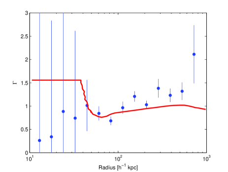
Figure 18: The adiabatic index deduced in this work (points with error bars), and the profile derived by Tozzi & Norman (2001) (solid curve).

5.7 The effect of the cD galaxy

Figures 13 and 16 show that the 2D and 3D temperature profiles peak at $r\sim 0.1r_{500}$ and decline at large radii. At smaller radii the temperature profile also declines. This decline of the temperature profile at small radii occurs within the region that includes emission from the cD galaxy. Since the gas in the cD is denser and colder than the cluster gas, it might be the cause for this decline at small radii. In order to evaluate the effect of the cD on the cluster we modeled the emission of the cD. We estimated the gas mass density profile by taking the profile of M87, which is the cD in the nearest cluster of galaxies. We thus fitted a double $\beta$ model (as Matsushita et al. 2002 did) to the surface brightness data in M87. The values of the best-fitted parameters of the gas number density of the cD are shown in table 7. Our obtained values agree well with the ones in Matsushita et al. (2002). For the evaluation of the cD mass profile we took $R_{e}=7.8$ h^-1 kpc, $r_{s}=10$ h^-1 kpc, $M_{\rm cD}=10^{13}$ $M_{\odot}$, and $M_{\rm stars}=5\cdot 10^{11}$ $M_{\odot}$ (for the mass profile see section 4.3).

Table 7: The values of the best fitted parameters of the gas number density of the cD assuming a double beta model for the gas mass density of cD. We fitted to the values taken from Matsushita et al. (2002)

Parameter	Value
$n_{e}(1,0)$ [$cm^{-3}$]	$0.117^{+0.016}_{-0.014}$
$r_{c,1}$ [arcmin]	$0.366^{+0.071}_{-0.064}$
$\beta_{1}$	$0.439^{+0.033}_{-0.025}$
$n_{e,2}(0)$ [$cm^{-3}$]	$6.3^{+0.8}_{-0.7}\cdot 10^{-3}$
$r_{c,2}$ [arcmin]	$5.41^{+0.31}_{-0.33}$
$\beta_{2}$	0.47(fixed)

We checked the innermost part of the cluster $r\lesssim 10$ h^-1 kpc. This is out of the data range and requires an extrapolation, so we extrapolated using particular profiles. We used NFW for the DM profile and a double $\beta$ model for the gas profile. In figure 19 we plot the emissivity of the cD galaxy and compare it to the emissivity of the cluster. The figure shows that the cD is dominant only at $r<4$ h^-1 kpc. Since the innermost surface brightness data point is at $4$ h^-1 kpc, the effect of the cD galaxy is likely minor, as expected in a rich cluster like A1689.

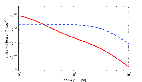
Figure 19: A comparison between the emissivity profiles of the cluster (dashed line) and of the cD galaxy (solid line). The cD emissivity profile is derived by assuming it is similar to that of M87.

We checked for an indication in the abundance profile that the cD contributes only at $<4$ h^-1 kpc (if at all). Note that the spatial resolution of Chandra is $\sim 0.5"$, which for the redshift of A1689 is $\sim 1.5$ h${}_{0.7}^{-1}$ kpc. Also the cD galaxy coincides with the X-ray centroid within $\sim 1.5"$ uncertainties (XW02). Figure 20 indicates that the abundance may be higher, $\sim 0.9$, in the core than in the outer region. However, this is not statistically significant due to the narrow annuli used which give high errors. The errors were calculated here after freezing the temperature and the normalization. If these parameters are allowed to vary, this will of course increase the errors in the abundance.

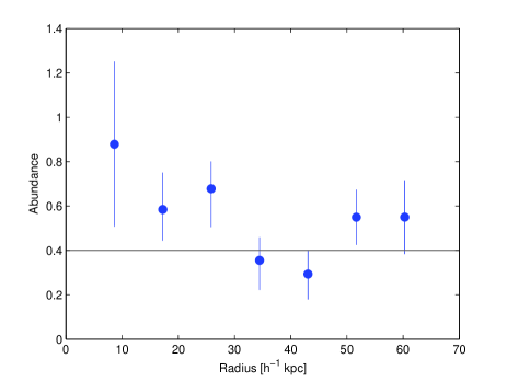
Figure 20: A comparison of the abundance (in solar units) within 4” annuli (points with error bars) to the average abundance of the cluster in a $3^{\prime}$ aperture (solid line). The errors may be underestimated (see text).

As expected from the low emissivity of the cD galaxy compared to that of the cluster, it is hard to see spectroscopically an indication of the cD. We fitted a double temperature model, WABS(MEKAL+MEKAL), to the $3^{\prime}$ aperture, where the abundance of the first component (the cD galaxy) was fixed to solar and the second (the cluster) to 0.4 solar (the average value in the cluster). We also fixed the Galactic absorption to be $2\cdot 10^{-20}$ cm^-2 as appropriate for this direction (Dickey & Lockman 1990). The resulting best fit is with two temperatures, a cold one $\sim 0.5$ keV and a hot one $\sim 10$ keV. This, however, might be due to the real multi-temperature nature of the cluster gas. Extracting a smaller region, where the cD flux should be less diluted by the cluster flux, gave about the same two temperatures but with high errors. Thus, spectroscopic fitting was inconclusive.

6 Discussion

The increasing quality of X-ray and optical imaging data motivates renewed and more thorough examinations of the physical nature of galaxy clusters as revealed by the very different processes of bremsstrahlung radiation and the gravitational deflection of light. In this paper we have examined the apparently relaxed cluster A1689, where only minimal substructure is evident from the dark matter, galaxy, and X-ray distributions and where the X-ray emission is smooth and symmetric. The longstanding claims of discrepancies in the total cluster mass estimated from these different kinds of analysis can now be investigated with greater precision, fewer assumptions, and in a more model-independent way.

There is a strong incentive to describe in analytical form the general nature of the total mass, gas, and temperature profiles. These quantities are inextricably bound up with the process of structure formation, including the nature of dark matter and the cooling history of the gas including interaction and merging of substructure. Thus, having an analytical form of the profiles is very useful. The most commonly examined profile for the dark matter, based on N-body simulations of collisionless dark matter, is the NFW profile. In contrast the most commonly fitted gas mass density or surface brightness profile, the $\beta$ model, is essentially empirically based. The temperature profile is often derived from the analytical expression of the gas density using the polytropic equation of state, or the gas is taken to be isothermal since the temperature gradient was undetectable with the old X-ray satellites. This way of analyzing the cluster can lead to substantial errors in the DM density, gas density, and temperature values and the derived quantities such as the overall mass.

As we discussed in the Introduction, the total mass profile can be independently determined from lensing measurements, or from X-ray measurements of the gas density and temperature profiles based on the assumption of hydrostatic equilibrium. (Clearly, the latter can be done also with spatially resolved S-Z measurements, when available.) The second basic assumption adopted in our analysis is spherical symmetry. Obviously, elongation along the line of sight is possible, but - as we have mentioned in the Introduction - this typically can introduce a 20% bias in the mass estimate. For a detailed discussion of the impact of triaxial cluster morphology, see Gavazzi (2005).

We have suggested here a model-independent method which uses free parameters and does not assume a specific profile for any mass component. The only hidden assumption is a linear (in log-log) interpolation between the free parameters; this just assumes a reasonable degree of smoothness in the profiles. The profiles are also extrapolated beyond the data, but we showed that the results are insensitive to the detailed extrapolation. We specifically used a simple power law extrapolation for both the total mass density and for the gas mass density, with the same power law index assumed in order to approach a constant gas fraction at large radii. Our model-independent method is the best way to obtain the values of the important parameters of clusters at radii where there are good quality data. Our model-independent method can and will be applied to joint analyses of measurements of other clusters.

Within the data range, the highest value of the 3D temperature (fig. 16) is 2–3 times higher than the lowest value. Specifically, the temperature profile peaks at $r\sim 0.1r_{500}$ and declines at both smaller and larger radii. The denser environment at the center of a cluster should naturally cause a decrease in the temperature there. We indeed find in this cluster that the 2D temperature decreases towards the center of the cluster, at $r<50-100$ $h^{-1}$ kpc (figure 13). This can be due to several mechanisms. First, the high gas number density in the center of the cluster causes a rapid loss of energy and a decrease in the temperature. As pressure support decreases, the gas should gravitate towards the bottom of the cluster potential well, i.e., the center of the cluster, in a so-called ”cooling flow” (Fabian 1994). A cooling flow should manifest in a detectable surface brightness enhancement in the X-ray emission from the central region of a cluster, $\sim 100-200$ kpc. Many studies have failed to find these cooling flows (MME99), at least not as expected in a simple or a standard cooling flow model (Fabian et al. 2001; Peterson et al. 2001). An explanation for this failure can be a more complicated mechanism which maybe includes reheating of the gas (e.g., by energetic particles; Rephaeli & Silk 1995), mixing, differential absorption, efficient conversion of cooling flow gas into low-mass stars, an inhomogeneous metallicity distribution (which is not the situation in A1689, at least not in terms of a radial gradient: fig. 2), or disruption of cooling flows by a recent subcluster merger (see discussion in Fabian et al. 2001; Peterson et al. 2001).

There are uncertainties about the criteria for finding cooling flows, and even with fixed criteria the decision whether cooling flows exist is still data dependent. At times the ”solution” has been to exclude the inner, problematic region. Finding the value of the gas mass density in the model-independent approach bypasses these two problems, the unknown physical processes and the data dependence, as it allows for an analysis with fewer prior assumptions. Another way to reduce the core temperature is through the effect of the cD galaxy that is often anchored at the cluster center. The cD galaxy has a lower temperature and is denser than the cluster so it can in principle be the main cause for the low temperature at the center. However, based on our our initial, limited study it seems unlikely that the cD has a major effect in A1689, since the emissivity of the cD dominates that of the cluster only below $r=4$ h^-1 kpc (fig. 19).

We have found a good fit to the observed 2D profiles of the lensing surface density and the X-ray surface brightness. Due to the smoothness of the profiles, we were able to fit the data with a relatively small number of free parameters. We have found a good agreement with previous results for all the parameters we have checked for A1689, including gas mass density, gas fraction profiles, measured temperature, adiabatic index, and abundance (except compared to AM04). The total mass density profile we obtained was essentially determined directly by the lensing data alone, with $\lesssim 1\%$ differences introduced by using the X-ray data as well. This is the case since we did not use the X-ray temperature as part of the fit.

We have shown that it is possible to obtain a model independent 3D mass profile for which very good agreement is found between the lensing mass profile and the X-ray emission profile. However, there is still a discrepancy between the temperature derived directly from (X-ray) measurements, and that deduced from a solution to the HEE, with the latter $\sim 30\%$ higher at all radii, as has already been determined by Mazzotta et al.(2004) and Rasia et al. (2005). Other phenomena, such as bulk motions, turbulence, and nonthermal degree of freedom may contribute to the pressure, and thus reduce the temperature with respect to the one obtained from assuming that thermal gas pressure is the only contributor. Specifically, Faltenbacher et al. (2005) claim that based on their high-resolution cosmological simulations - in which they identified and analyzed eight clusters at $z=0$ - about 10% of the total pressure support may be contributed by random gas bulk motions, which may affect temperature by up to 20%. It has also been suggested that X-ray luminous clumps of relatively low temperature may bias projected temperature measurements downward (Kawahara et al. 2006). In any case, as we have already mentioned this temperature discrepancy is much smaller than the mass discrepancy by a factor of $2-4$ encountered in previous (separate X-ray and lensing) analyses.

The derived entropy profile for A1689 has a power law form with no obvious central flattening, at least at $r>0.02r_{\rm vir}$, as expected for massive clusters from theoretical work (Tozzi & Norman 2001). The existence and the level of the entropy floor is still not completely clear in simulations, since different simulation methods give different results (Voit, Kay, & Bryan 2005). This is probably due to the limited resolution of simulations which is especially critical in the core of the cluster. Upcoming simulations with spatial resolution of $\sim 5$ kpc should give a better understanding of the entropy floor. Our derived radial slope is around $0.8$ rather than $1.1$, flatter than the prediction. Since using simple parametrized models for the DM and the gas gave a power law index of $1.1$, we believe the value of $0.8$ might be a more accurate result, which might be a reflection of a more complex gas dynamics and preheating history. Indeed, it has been suggested from simulations that preheating decreases the power law index in the region of our data (Borgani et al. 2005).

Appendix A Corrleations between parameter values

In our model-independent approach we have determined parameter values by fitting the projected mass, gas density, and temperature. Projection of the 3D quantities builds up correlations between their best-fit values in different radial bins. An illustration of the degree of such correlations is shown in table A1, which is the correlation matrix of the free parameters, taken from running four and nine free parameters for the total and gas mass density respectively. The correlation in the deduced 2D temperature is shown in table A2. The elements of the 2D temperature correlation matrix correspond to the 12 values of the 2D radii (fig. 13). In both tables the correlations are quite strong between adjacent elements. In the 2D temperature correlation matrix there are also strong correlations between elements which are not adjacent but are at small radii, i.e. the upper left part of the table.

Table 8: The $13\times 13$ correlation matrix for $i=4$, $j=9$ free parameters for the total mass and gas mass density, respectively.

	i=1	i=2	i=3	i=4	j=1	j=2	j=3	j=4	j=5	j=6	j=7	j=8	j=9
i=1	1.000	-0.342	0.197	-0.072	-0.026	0.036	0.034	0.028	0.040	0.026	0.026	0.001	-0.006
i=2	-0.342	1.000	-0.825	0.273	0.004	-0.005	-0.000	0.010	-0.008	-0.051	-0.074	-0.005	0.019
i=3	0.197	-0.825	1.000	-0.599	-0.002	0.002	-0.000	-0.005	0.030	0.075	0.091	-0.001	0.004
i=4	-0.072	0.273	-0.599	1.000	0.001	-0.002	-0.002	-0.003	-0.028	-0.045	-0.038	0.018	-0.074
j=1	-0.026	0.004	-0.002	0.001	1.000	-0.749	0.323	-0.152	0.057	-0.026	0.010	-0.003	0.002
j=2	0.036	-0.005	0.002	-0.002	-0.749	1.000	-0.613	0.266	-0.106	0.047	-0.018	0.006	-0.003
j=3	0.034	-0.000	-0.000	-0.002	0.323	-0.613	1.000	-0.643	0.238	-0.107	0.042	-0.014	0.007
j=4	0.028	0.010	-0.005	-0.003	-0.152	0.266	-0.643	1.000	-0.560	0.234	-0.095	0.031	-0.014
j=5	0.040	-0.008	0.030	-0.028	0.057	-0.106	0.238	-0.560	1.000	-0.590	0.223	-0.075	0.038
j=6	0.026	-0.051	0.075	-0.045	-0.026	0.047	-0.107	0.234	-0.590	1.000	-0.557	0.174	-0.086
j=7	0.026	-0.074	0.091	-0.038	0.010	-0.018	0.042	-0.095	0.223	-0.557	1.000	-0.492	0.226
j=8	0.001	-0.005	-0.001	0.018	-0.003	0.006	-0.014	0.031	-0.075	0.174	-0.492	1.000	-0.689
j=9	-0.006	0.019	0.004	-0.074	0.002	-0.003	0.007	-0.014	0.038	-0.086	0.226	-0.689	1.000

Table 9: The $12\times 12$ correlation matrix of the deduced 2D temperature for $i=4$, $j=9$ free parameters for the total mass and gas mass density, respectively. The raw and column numbers specify radial points (see fig. 13).

1.0000	0.9085	-0.6717	0.2874	-0.1372	-0.0423	0.0604	-0.0008	-0.0233	-0.0026	0.0050	-0.0005
0.9085	1.0000	-0.3046	0.1364	-0.0854	-0.0382	0.0264	0.0081	-0.0008	0.0044	0.0100	0.0093
-0.6717	-0.3046	1.0000	-0.3047	0.1225	0.0123	-0.0773	0.0206	0.0515	0.0162	0.0111	0.0219
0.2874	0.1364	-0.3047	1.0000	-0.3307	-0.1412	0.1199	0.0292	-0.0119	0.0156	0.0363	0.0304
-0.1372	-0.0854	0.1225	-0.3307	1.0000	0.2272	-0.3406	0.0566	0.1892	0.0501	0.0213	0.0626
-0.0423	-0.0382	0.0123	-0.1412	0.2272	1.0000	0.8048	0.0974	-0.1890	0.0403	0.1515	0.0908
0.0604	0.0264	-0.0773	0.1199	-0.3406	0.8048	1.0000	0.3025	-0.0556	0.0577	0.1344	0.1047
-0.0008	0.0081	0.0206	0.0292	0.0566	0.0974	0.3025	1.0000	0.9125	0.2147	0.0351	0.2234
-0.0233	-0.0008	0.0515	-0.0119	0.1892	-0.1890	-0.0556	0.9125	1.0000	0.4082	0.1285	0.2108
-0.0026	0.0044	0.0162	0.0156	0.0501	0.0403	0.0577	0.2147	0.4082	1.0000	0.6956	0.2024
0.0050	0.0100	0.0111	0.0363	0.0213	0.1515	0.1344	0.0351	0.1285	0.6956	1.0000	0.7934
-0.0005	0.0093	0.0219	0.0304	0.0626	0.0908	0.1047	0.2234	0.2108	0.2024	0.7934	1.0000

References

- Allen (1998) Allen, S. W. 1998, MNRAS , 296, 392
- Andersson & Madejski (2004) Andersson, K. E., & Madejski, G. M. 2004, ApJ , 607, 190 (AM04)
- Arieli, Rephaeli & Norman (2008) Arieli, Y., Rephaeli, Y., & Norman, M. L. 2008, in preparation
- Arnalte Mur et al. (2006) Arnalte Mur, P., Ellis, S. C., & Colless, M. 2006, Publications of the Astronomical Society of Australia, 23, 33
- Bohringer et al. (1994) Bohringer, H., Briel, U. G., Schwarz, R. A., Voges, W., Hartner, G., & Trumper, J. 1994, Nature , 368, 828
- Borgani et al. (2002) Borgani, S., Governato, F., Wadsley, J., Menci, N., Tozzi, P., Quinn, T., Stadel, J., & Lake, G. 2002, MNRAS , 336, 409
- Borgani et al. (2005) Borgani, S., Finoguenov, A., Kay, S. T., Ponman, T. J., Springel, V., Tozzi, P., & Voit, G. M. 2005, MNRAS , 361, 233
- Bradač et al. (2006) Bradač, M., et al. 2006, ApJ , 652, 937
- Broadhurst et al. (1995) Broadhurst, T. J., Taylor, A. N., & Peacock, J. A. 1995, ApJ , 438, 49
- Broadhurst et al. (2005) Broadhurst, T., et al. 2005, ApJ , 621, 53
- Broadhurst et al. (2005) Broadhurst, T., Takada, M., Umetsu, K., Kong, X., Arimoto, N., Chiba, M., & Futamase, T. 2005, Ap. J. Lett. , 619, L143
- Brown & Bregman (2001) Brown, B. A., & Bregman, J. N. 2001, ApJ , 547, 154
- Bullock et al. (2001) Bullock, J. S., Kolatt, T. S., Sigad, Y., Somerville, R. S., Kravtsov, A. V., Klypin, A. A., Primack, J. R., & Dekel, A. 2001, MNRAS , 321, 559
- Cavaliere et al. (2005) Cavaliere, A., Lapi, A., & Rephaeli, Y. 2005, ApJ , 634, 784
- Clowe et al. (2004) Clowe, D., Gonzalez, A., & Markevitch, M. 2004, ApJ , 604, 596
- Clowe et al. (2006) Clowe, D., Bradač, M., Gonzalez, A. H., Markevitch, M., Randall, S. W., Jones, C., & Zaritsky, D. 2006, Ap. J. Lett. , 648, L109
- Clowe & Schneider (2001) Clowe, D., & Schneider, P. 2001, A&A , 379, 384
- Czoske et al. (2002) Czoske, O., Moore, B., Kneib, J.-P., & Soucail, G. 2002, A&A , 386, 31
- Dickey & Lockman (1990) Dickey, J. M., & Lockman, F. J. 1990, , 28, 215
- Dupke et al. (2007) Dupke, R. A., Mirabal, N., Bregman, J. N., & Evrard, A. E. 2007, ApJ , 668, 781
- Dye et al. (2001) Dye, S., Taylor, A. N., Thommes, E. M., Meisenheimer, K., Wolf, C., & Peacock, J. A. 2001, MNRAS , 321, 685
- Fabian (1994) Fabian, A. C. 1994, , 32, 277
- Fabian et al. (2001) Fabian, A. C., Mushotzky, R. F., Nulsen, P. E. J., & Peterson, J. R. 2001, MNRAS , 321, L20
- Faltenbacher et al. (2005) Faltenbacher, A., Kravtsov, A. V., Nagai, D., & Gottlöber, S. 2005, MNRAS , 358, 139
- Franx et al. (1997) Franx, M., Illingworth, G. D., Kelson, D. D., van Dokkum, P. G., & Tran, K.-V. 1997, Ap. J. Lett. , 486, L75
- Frye & Broadhurst (1998) Frye, B., & Broadhurst, T. 1998, Ap. J. Lett. , 499, L115
- Frye et al. (2002) Frye, B., Broadhurst, T., & Benítez, N. 2002, ApJ , 568, 558
- Gavazzi et al. (2003) Gavazzi, R., Fort, B., Mellier, Y., Pelló, R., & Dantel-Fort, M. 2003, A&A , 403, 11
- Gavazzi et al. (2004) Gavazzi, R., Mellier, Y., Fort, B., Cuillandre, J.-C., & Dantel-Fort, M. 2004, A&A , 422, 407
- Gavazzi (2005) Gavazzi, R. 2005, A&A , 443, 793
- Grego et al. (2001) Grego, L., Carlstrom, J. E., Reese, E. D., Holder, G. P., Holzapfel, W. L., Joy, M. K., Mohr, J. J., & Patel, S. 2001, ApJ , 552, 2
- Hallman et al. (2007) Hallman, E. J., Burns, J. O., Motl, P. M., & Norman, M. L. 2007, ApJ , 665, 911
- Hayashi & White (2006) Hayashi, E., & White, S. D. M. 2006, MNRAS , 370, L38
- Hennawi et al. (2007) Hennawi, J. F., Dalal, N., Bode, P., & Ostriker, J. P. 2007, ApJ , 654, 714
- Hernquist (1990) Hernquist, L. 1990, ApJ , 356, 359
- Jannuzi et al. (1997) Jannuzi, B. T., Yanny, B., & Impey, C. 1997, ApJ , 491, 146
- Jee et al. (2007) Jee, M. J., et al. 2007, ApJ , 661, 728
- Jing & Suto (2002) Jing, Y. P., & Suto, Y. 2002, ApJ , 574, 538
- Kaiser (1991) Kaiser, N. 1991, ApJ , 383, 104
- Kawahara et al. (2007) Kawahara, H., Suto, Y., Kitayama, T., Sasaki, S., Shimizu, M., Rasia, E., & Dolag, K. 2007, ApJ , 659, 257
- King et al. (2002) King, L. J., Clowe, D. I., & Schneider, P. 2002, A&A , 383, 118
- Kneib et al. (2003) Kneib, J.-P., et al. 2003, ApJ , 598, 804
- Lloyd-Davies et al. (2000) Lloyd-Davies, E. J., Ponman, T. J., & Cannon, D. B. 2000, MNRAS , 315, 689
- Markevitch et al. (1999) Markevitch, M., Vikhlinin, A., Forman, W. R., & Sarazin, C. L. 1999, ApJ , 527, 545
- Markevitch et al. (2002) Markevitch, M., Gonzalez, A. H., David, L., Vikhlinin, A., Murray, S., Forman, W., Jones, C., & Tucker, W. 2002, Ap. J. Lett. , 567, L27
- Markevitch et al. (2004) Markevitch, M., Gonzalez, A. H., Clowe, D., Vikhlinin, A., Forman, W., Jones, C., Murray, S., & Tucker, W. 2004, ApJ , 606, 819
- Katgert et al. (2004) Katgert, P., Biviano, A., & Mazure, A. 2004, ApJ , 600, 657
- Matsushita et al. (2002) Matsushita, K., Belsole, E., Finoguenov, A., Bohringer, H. 2002, A&A , 386, 77
- Mazzotta et al. (2004) Mazzotta, P., Rasia, E., Moscardini, L., & Tormen, G. 2004, MNRAS , 354, 10
- Medezinski et al. (2007) Medezinski, E., et al. 2007, ApJ , 663, 717
- Milosavljević et al. (2007) Milosavljević, M., Koda, J., Nagai, D., Nakar, E., & Shapiro, P. R. 2007, Ap. J. Lett. , 661, L131
- Miralda-Escude & Babul (1995) Miralda-Escude, J., & Babul, A. 1995, ApJ , 449, 18
- Mohr et al. (1999) Mohr, J. J., Mathiesen, B., & Evrard, A. E. 1999, ApJ , 517, 627 (MME99)
- Mushotzky & Scharf (1997) Mushotzky, R. F., & Scharf, C. A. 1997, Ap. J. Lett. , 482, L13
- Oguri et al. (2005) Oguri, M., Takada, M., Umetsu, K., & Broadhurst, T. 2005, ApJ , 632, 841
- Okabe & Umetsu (2007) Okabe, N., & Umetsu, K. 2007, ArXiv Astrophysics e-prints, arXiv:astro-ph/0702649
- Peterson et al. (2001) Peterson, J. R., et al. 2001, A&A , 365, L104
- Pettini et al. (2001) Pettini, M., Shapley, A. E., Steidel, C. C., Cuby, J.-G., Dickinson, M., Moorwood, A. F. M., Adelberger, K. L., & Giavalisco, M. 2001, ApJ , 554, 981
- Ponman et al. (2003) Ponman, T. J., Sanderson, A. J. R., & Finoguenov, A. 2003, MNRAS , 343, 331
- Randall et al. (2007) Randall, S. W., Markevitch, M., Clowe, D., Gonzalez, A. H., & Bradac, M. 2007, ArXiv e-prints, 704, arXiv:0704.0261
- Rasia et al. (2005) Rasia, E., Mazzotta, P., Borgani, S., Moscardini, L., Dolag, K., Tormen, G., Diaferio, A., & Murante, G. 2005, Ap. J. Lett. , 618, L1
- Rephaeli & Silk (1995) Rephaeli, Y., & Silk, J. 1995, ApJ , 442, 91
- Romanowsky et al. (2003) Romanowsky, A. J., Douglas, N. G., Arnaboldi, M., Kuijken, K., Merrifield, M. R., Napolitano, N. R., Capaccioli, M., & Freeman, K. C. 2003, Science, 301, 1696
- Sanderson et al. (2003) Sanderson, A. J. R., Ponman, T. J., Finoguenov, A., Lloyd-Davies, E. J., & Markevitch, M. 2003, MNRAS , 340, 989
- Sharon et al. (2005) Sharon, K., Broadhurst, T. J., Benitez, N., Coe, D., Ford, H., & ACS Science Team 2005, Gravitational Lensing Impact on Cosmology, 225, 167
- Silk (2003) Silk, J. 2003, MNRAS , 343, 249
- Taylor et al. (1998) Taylor, A. N., Dye, S., Broadhurst, T. J., Benitez, N., & van Kampen, E. 1998, ApJ , 501, 539
- Tozzi & Norman (2001) Tozzi, P., & Norman, C. 2001, ApJ , 546, 63
- Tyson & Fischer (1995) Tyson, J. A., & Fischer, P. 1995, Ap. J. Lett. , 446, L55
- Vikhlinin (2006) Vikhlinin, A. 2006, ApJ , 640, 710
- Vikhlinin et al. (2005) Vikhlinin, A., Markevitch, M., Murray, S. S., Jones, C., Forman, W., & Van Speybroeck, L. 2005, ApJ , 628, 655
- Voigt & Fabian (2006) Voigt, L. M., & Fabian, A. C. 2006, MNRAS , 368, 518
- Voit et al. (2003) Voit, G. M., Balogh, M. L., Bower, R. G., Lacey, C. G., & Bryan, G. L. 2003, ApJ , 593, 272
- Voit (2005) Voit, G. M. 2005, Reviews of Modern Physics, 77, 207
- Voit et al. (2005) Voit, G. M., Kay, S. T., & Bryan, G. L. 2005, MNRAS , 364, 909
- Wu & Fang (1997) Wu, X.-P., & Fang, L.-Z. 1997, ApJ , 483, 62
- Wu et al. (1998) Wu, X.-P., Chiueh, T., Fang, L.-Z., & Xue, Y.-J. 1998, MNRAS , 301, 861
- Xue & Wu (2002) Xue, S.-J., & Wu, X.-P. 2002, ApJ , 576, 152 (XW02)