Stability of liquid ridges on chemical micro- and nanostripes

Abstract

We analyze the stability of sessile filaments (ridges) of nonvolatile liquids versus pearling in the case of externally driven flow along a chemical stripe within the framework of the thin film approximation. The ridges can be stable with respect to pearling even if the contact line is not completely pinned. A generalized stability criterion for moving contact lines is provided. For large wavelengths and no drive, within perturbation theory, an analytical expression of the growth rate of pearling instabilities is derived. A numerical analysis shows that drive further stabilizes the ridge by reducing the growth rate of unstable perturbations, even though there is no complete stabilization. Hence the stability criteria established without drive ensure overall stability.

I Introduction

In the last decade substantial efforts have been invested in integrating chemical processes into microfluidic systems known as “labs on a chip” stone01 ; mitchell01 ; giordano01 . These microfluidic devices do not only allow for cheap mass production but they can also operate with much smaller quantities of reactants and reaction products than standard laboratory equipments.

In this context both closed and open channel systems are considered for fluid transport. While closed channels are prone to clogging by, e.g., colloids or large biopolymers, the fluid in open channel systems has less friction because it is in contact with less substrate material, and production is possibly cheaper. The substrate surfaces can be structured chemically by printing or photographic techniques. Conceptually, the liquid is guided by lyophilic stripes on an otherwise lyophobic substrate gau99 ; darhuber01 ; dietrich05 ; zhao02 , i.e., it is confined by laterally varying substrate potentials, acting as “chemical walls”.

Here we analyze the stability of homogeneously filled chemical channels with respect to pearling, i.e., breakup into a string of droplets. For all contact angles, on homogeneous substrates sessile filaments (ridges) of nonvolatile liquids are unstable with respect to pearling, even in the presence of line tension brinkmann02 ; brinkmann05 ; mechkov07 . However, in the cases that the contact line is infinitely stiff or pinned, e.g., at the edges of a chemical channel formed by a lyophilic stripe on an otherwise lyophobic substrate, the instability is suppressed if the contact angle of the liquid-vapor interface with the substrate is smaller than $90^{\circ}$ davis80 ; brinkmann04 . Molecular dynamics simulations have confirmed this even at the nano-scale koplik06a .

From these results it is not clear whether complete pinning is required to stabilize a liquid ridge. In an actual sample the three phase contact angle will not vary step-like at the channel edge. One rather expects a gradual transition, which leads to a partial stabilization: the contact line can move but the lateral variation of the effective contact angle will impose a restoring force.

In this paper we use a mesoscopic hydrodynamic model to describe a nonvolatile fluid on a chemical stripe with such partial stabilization by realistic (i.e., not step-like) edges. We use a numerical scheme based on the thin film approximation, assuming a sharp liquid-gas interface, partial wetting on both the stripe and the embedding substrate, small contact angles, and smooth lateral variations of the disjoining pressure. Analytical estimates can be obtained within appropriate macroscopic approximations, the validity of which we discuss in the context of finite size issues.

In accordance with King et al. king06 , without drive and on a homogeneous substrate we find that cylinder-like sessile ridges are stationary but prone to a Rayleigh-Plateau type pearling instability. We generalize the analytical macroscopic stability criterion for liquid ridges on chemical channels with sharp boundaries brinkmann02 ; gau99 to the case of smooth chemical steps. A linear stability analysis allows us to account for the occurrence of large-wavelength pearling, both numerically and analytically. The presence of a chemical stripe partially stabilizes the ridge with respect to pearling. The analytical criterion for the stability of a pinned ridge is in good accordance with the stability domain found numerically. We also find a quantitative agreement between the growth rate of long-wavelength pearling obtained from numerical stability analysis and its corresponding analytical expression obtained by a perturbative analysis.

External drive applied along the ridge always has an overall stabilizing effect. However, drive never completely stabilizes an unstable liquid ridge but merely shifts the domain of unstable modes to larger wave lengths.

In the next section II we introduce the system we consider as well as the numerical method we use, along with a discussion of finite size effects. In Sec. III we introduce the dimensionless thin film equation and the parametrization of the chemical stripe. We analyze the stationary solutions in Sec. IV and their linear stability in Sec. V. We summarize and conclude in Sec. VI.

II Description of the system

Figure 1: Schematic view of the investigated system. The substrate is topographically flat, invariant in the $y$ direction, chemically heterogeneous and $2\,L$-periodic in the $x$ direction. A liquid ridge forms above the lyophilic stripe (grey) of width $2\,x_{0}$ centered on the $y$-axis and a wetting film covers the surrounding lyophobic regions (black). A body force aligned with the $y$-axis (caused, e.g., by a substrate tilt) generates flow along the stripe. The local film thickness at time $t$ is given by $\tilde{H}(x,y,t)$. Depending on the characteristics of the chemical stripe, the ridge may be subject to pearling instabilities (exaggerated).

As illustrated in Fig. 1 we consider a viscous, incompressible, and nonvolatile fluid on a partially wetting substrate featuring a straight “chemical channel”, i.e., a lyophilic stripe with macroscopic axial extension separating two lyophobic domains. The equilibrium contact angle is smaller on the channel than on the surrounding, macroscopically wide, homogeneous substrate. For reasons given below, our analysis requires a finite spatial extent $2\,L$ in the transverse $x$ direction. For convenience we assume periodic boundary conditions at $x=\pm L$ . $L$ is taken to be large enough so that the stripe of width $2\,x_{0}$ can be considered as isolated. In this “chemical channel” a liquid ridge of local thickness can be formed if the amount of liquid is sufficiently large. The local thickness $\widetilde{H}(x,y,t)$ includes possible variations in the vicinity of the ridge-like stationary solution.

For such a configuration, the film has an almost uniform thickness $H_{\text{film}}=\widetilde{H}(\pm L,y,t)$ far from the stripe and one can define the excess cross sectional area

$$V_{\text{ex}}\left(x,y\right)=\int_{-L}^{L}\mathrm{d}x\left[\widetilde{H}(x,y,t)-H_{\text{film}}\right]$$ (1)

of the liquid in the channel. For $y$-invariant stationary solutions this quantity corresponds to the excess volume of liquid per unit length on top of the wetting film and thus adequately characterizes the extra amount of liquid in the system independently of the finite lateral size $2\,L$.

We consider a finite lateral system size for the following reason. Given a configuration in which a macroscopic ridge is in stable mechanical equilibrium with the wetting film on a substrate of finite width, extending the system size $2\,L$ at constant excess cross-section eventually leads to an unstable configuration: upon transferring liquid from the ridge into the wetting film the pressure inside the ridge increases more than in the wetting film and the ridge will drain into the film. Therefore the only globally stable configuration on arbitrarily large substrates is a basically flat wetting film with a slightly increased thickness above the channel bauer99d .

Thus the existence of stable ridges is formally a pure finite size effect. However, as will be discussed in Sec. IV, the limit of stability versus pearling at a given system size can correspond to a width of the ridge which is small with respect to the lateral extent of the system. Hence there is a wide range of configurations for which the quantities relevant for the dynamics of the ridge are primarily determined by macroscopic quantities such as the excess cross-section $V_{\mathrm{ex}}$, which do not depend on the system size.

Within our approach the thin film around the liquid ridge plays an auxiliary role. It facilitates the mobility of the edges of the ridge, but contributes negligibly to the dynamics within an appropriately chosen range of configurations.

A body force aligned with the channel (e.g., gravity if the substrate is tilted as illustrated in Fig. 1 — the component normal to the substrate can be neglected) drives the liquid along the chemical stripe. Our goal is to establish and discuss both analytically and numerically the conditions of linear stability of a driven flow in a homogeneously filled channel, in particular with respect to pearling.

Since liquid ridges with contact angles larger than $90^{\circ}$ are unstable even for pinned contact lines, we restrict our analysis to small contact angles using the thin film approximation oron97 . As will be shown below, the translational invariance of the base state effectively reduces the corresponding boundary value problem to a set of ordinary differential equations for the base state and to an eigenvalue problem for ordinary differential equations for the linear stability analysis. An analytical analysis is possible in the limit of large wavelengths of the pearling perturbation and without drive.

In the general case, we solve the equations numerically using the software Auto2000 auto . Within this numerical approach, instead of looking for a non-trivial solution in a complicated system, one starts with a simple configuration for which the solution is known. In the present case the latter is a flat wetting film on a homogeneous substrate. By gradually incrementing the system parameters towards non-trivial values, one is able to explore a domain of non-trivial solutions containing the simple starting point. In the present case, the most important system parameters are the chemical contrast between the channel and the embedding substrate, the excess cross-section, drive, and the wavenumber of the perturbation. As for the explicit dependence of the substrate heterogeneity on the lateral coordinate $x$, treating $x$ as a part of the solution vector renders the system autonomous as required by Auto2000.

III Thin film dynamics

In the limit of small gradients (i.e., long wavelengths), the dynamics of a thin film of a Newtonian, nonvolatile viscous liquid is well described by the standard thin film equation for the local film thickness $\tilde{H}(x,y,t)$ (see, e.g., Ref. oron97 ). In view of future purposes, we decompose it into a conservation equation (2a), an expression (2b) for the lateral flow $\mathbf{\tilde{J}}$, and an equation (2c) for the local pressure $\tilde{P}$ :

$$\frac{\partial\tilde{H}\left(x,y,t\right)}{\partial t} = -\mathbf{\nabla}\cdot\tilde{\mathbf{J}}\left[x,\tilde{H}\left(x,y,t\right)\right]\,,$$ (2a)

$$\tilde{\mathbf{J}}\left(x,\tilde{H}\right) = -\frac{Q(\tilde{H})}{\eta}\mathbf{\nabla}\left[\tilde{P}(x,\tilde{H})-\rho gy\right]\,,$$ (2b)

$$\tilde{P}\left(x,\tilde{H}\right) = -\Pi(x,\tilde{H})-\sigma\mathbf{\nabla}^{2}\tilde{H}\,.$$ (2c)

The pressure in Eq. (2c) is the sum of the Laplace pressure, which is proportional to the surface tension coefficient $\sigma$, and the disjoining pressure $\Pi(x,\tilde{H})=-\partial\Phi(x,\tilde{H})/\partial\tilde{H}$. We choose [c.f. Eq. (3)] the same functional form for the effective interface potential $\Phi(x,\tilde{H})$ as frequently used in the context of wetting phenomena (see, e.g., Ref. degennes85 and Refs. dietrich88 and dietrich91 for refined versions). However, the effective interface potential is an equilibrium concept and the dynamics in a wetting film a few molecular layers thick is certainly not given by hydrodynamical equations. In this sense the repulsive part of $\Pi$ (or $\Phi$) serves the purpose of keeping the liquid film thickness nonzero even on the lyophobic substrate and thus allows the three phase contact line to move even in the absence of hydrodynamic slip at the liquid-substrate interface. Moreover, as described below, the variation of the contact angle between the channel and the substrate is encoded in the $x$-dependence of $\Phi$. The third aspect taken care of by $\Phi$ is to include the influence of long-ranged dispersion forces on the dynamics in the channel. Thus we do not expect Eq. (2) to be an accurate description of the microscopic dynamics near the contact line and in the wetting layer; rather, it bears some conceptual similarities with a phase field equation (a numerical method introduced in the context of crystal growth, see, e.g., Ref. langer80 ) for the three phase contact line. In particular, here it is not necessary to take the location of the edge into account explicitly. Also, since we do not discuss wetting transitions within this model, we do not expect a strong dependence of our results on details of $\Phi$, in particular not on the precise form of its short-ranged repulsive part and of other subdominant terms.

The additional pressure term $\rho\,g\,y$ in Eq. (2b) models the applied drive with acceleration $g$ of the mass density $\rho$. The mobility factor $\frac{Q(\tilde{H})}{\eta}=\frac{\tilde{H}^{3}}{3\eta}$ results from the integration of the Poiseuille type velocity profile over the vertical coordinate. Here we neglect drag by a vapor phase on the liquid-vapor interface and slip at the substrate noslip .

The thickness $\tilde{H}$, the pressure $\tilde{P}$, and the flow $\tilde{\mathbf{J}}$ depend on the transverse coordinate $x$. Since the chemical heterogeneity of the substrate is symmetric with respect to $x=0$ and the driving force is aligned with the $y$ axis, the stationary configurations exhibit the same symmetry.

Here we focus on the symmetric pearling mode (see Fig. 1) and thus we consider only the interval $x\in[0,L]$. Due to symmetry and the $2L$-periodicity, odd-order derivatives of the film thickness with respect to $x$ vanish at $x=0$ and $x=L$, for both the stationary profile and the perturbation.

In the following the viscosity $\eta$, the surface tension $\sigma$, and the mass density $\rho$ can be set to 1 by rescaling time, the lateral coordinates $(x,y)$, and the drive, respectively drive . The remaining degree of freedom, i.e., the scale of the vertical coordinate, is used to set a certain thickness to 1, which simplifies the expressions of $\Phi$ and $\Pi$ appearing in our model (see below).

The effective interface potential we use to model partial wetting is a two-term power law with attraction ($A(x)>0$) at long range and repulsion ($B(x)>0$) at short range:

$$\Phi\left(x,\tilde{H}\right)=-\frac{1}{2}\frac{A(x)}{\widetilde{H}^{2}}+\frac{1}{8}\frac{B(x)}{\widetilde{H}^{8}}.$$ (3)

The two terms follow from integrating the liquid-liquid and liquid-substrate Lennard-Jones pair potentials dietrich91 , assuming a homogenous substrate. We model a chemically inhomogeneous substrate by effective amplitudes $A(x)$ and $B(x)$, accounting for a local equilibrium wetting film thickness $a(x)=\left[\frac{B(x)}{A(x)}\right]^{1/6}$ and an ensuing effective local contact angle dietrich88

$$\theta_{\mathrm{eq}}(x)=\arccos\left\{1+\Phi\left[x,a\left(x\right)\right]/\sigma\right\}\\ =\arccos\left\{1-\frac{3A(x)}{8\sigma\left[a(x)\right]^{2}}\right\}\,.$$ (4)

Since in the present study we do not assign a quantitative meaning to the residual film but use it in order to facilitate contact line mobility, for numerical convenience we choose $B(x)\propto A(x)$, so that $a=\mathrm{const}$ is uniform over the whole substrate. According to Eq. (4) the contact angle contrast is then provided by the amplitude $A(x)$, which we refer to as the Hamaker constant, incorporating the commonly used prefactor $\left(6\pi\right)^{-1}$ degennes85 ; dietrich88 . Thus, within our model for the chemical heterogeneity and the thin film approximation, Young’s law provides a local relation between the equilibrium contact angle and the Hamaker constant:

$$A(x)=\frac{4}{3}a^{2}\sigma\left[\theta_{\text{eq}}(x)\right]^{2}\,.$$ (5)

In order to describe a chemical channel we choose $A(x)$ to be a smooth, $2\,L$-periodic function of the transverse coordinate $x$, symmetric around $x=0$, with well-defined plateau values both inside the stripe ($A_{\text{in}}$ for $\left|x\right|\ll x_{0}$) and on the surrounding substrate ($A_{\text{out}}$ for $x_{0}\ll\left|x\right|$). At the edges of the stripe, $A(x)$ varies smoothly over an effective step width $w$. A chemical channel is thus characterized by the stripe width $2\,x_{0}$, the step width $w$, and the chemical contrast $A_{\text{out}}-A_{\text{in}}$. For the subsequent numerical analysis we choose the following explicit functional form for $A(x)$:

$$A(x) = A_{\text{in}}+\frac{A_{\text{out}}-A_{\text{in}}}{2}\left[1-\tanh f(x)\right]$$ (6a)

$$f(x) = 2L\frac{\cos\frac{\pi x}{L}-\cos\frac{\pi x_{0}}{L}}{\pi w\sin\frac{\pi x_{0}}{L}}.$$ (6b)

The corresponding structure of the chemical step near the channel edge is illustrated in Fig. 2.

Figure 2: Present model of the chemical step of width $w=1$ with $A_{\text{out}}=4$ and $A_{\text{in}}=1$ as used in the numerical analysis. In the limiting case of infinite lateral extent $2L$, Eq. (6b) reduces to $f(x)=2\frac{x-x_{0}}{w}$. (a) Effective interface potential $\Phi$ and disjoining pressure $\Pi$ at the channel center $x=0$ [see Eqs. (6b), (8), and (10)]. (b) Laterally varying amplitude $A(x)$ as defined in Eq. (6). (c) Contour plot of the effective interface potential $\Phi$ near the channel edge. Note that the position $\tilde{H}=1$ of the minimum of $\Phi$ as a function of $\tilde{H}$ is independent of $x$.

In order to rescale the thin film equation, we take the residual film thickness $a$ as the vertical length scale of the problem so that in these units $\Phi$ attains its minimum at $\tilde{H}=1$. We also take $A_{\mathrm{in}}$ as a reference Hamaker constant. Equations (2a-c) then yield a lateral length scale $\lambda=a^{2}\sqrt{\sigma/A_{\mathrm{in}}}$, a pressure scale $A_{\mathrm{in}}/a=\sigma a/\lambda^{2}$, a time scale $\tau=\frac{\eta\,\lambda^{4}}{\sigma\,a^{3}}$, an acceleration scale $\gamma=\frac{\sigma\,a}{\rho\,\lambda^{3}}$, and a scale factor for the slopes: $\delta=\frac{a}{\lambda}\ll 1$. We note that these scales, just like $a$ and $A_{\mathrm{in}}$, are arbitrary (but suitable) and merely provide a consistent way to render the equations dimensionless with a minimal set of independent system parameters left. For example, the lateral length scale $\lambda$ is given by $\lambda=\sqrt{6}\xi_{\parallel}$, where $\xi_{\parallel}=\sqrt{\sigma/\frac{\partial^{2}\Phi}{\partial\tilde{H}^{2}}(a)}$ is the lateral correlation length of the interfacial height-height correlation function in thermal equilibrium dietrich88 .

Accordingly, in the following all quantities are dimensionless (i.e., effectively, $\sigma$, $\eta$, and $\rho$ are set to 1). In order to avoid clumsy notations from now on we use the same symbols for the dimensionless quantities so that the dimensionless evolution equation is given by

$$\frac{\partial\widetilde{H}\left(x,y,t\right)}{\partial t} = -\mathbf{\nabla}\cdot\widetilde{\mathbf{J}}\left[x,\widetilde{H}\left(x,y,t\right)\right]$$ (7a)

$$\widetilde{\mathbf{J}}\left(x,\widetilde{H}\right) = -Q(\widetilde{H})\,\mathbf{\nabla}\left[\widetilde{P}(x,\widetilde{H})-g\,y\right]$$ (7b)

$$\widetilde{P}\left(x,\widetilde{H}\right) = -\Pi(x,\widetilde{H})-\mathbf{\nabla}^{2}\widetilde{H}$$ (7c)

where $\Pi$ and $Q$ are defined as

$$\Pi\left(x,\tilde{H}\right)=-\frac{\partial\Phi}{\partial\widetilde{H}}=-A(x)\left(\frac{1}{\widetilde{H}^{3}}-\frac{1}{\widetilde{H}^{9}}\right)$$ (8)

and

$$Q=\widetilde{H}^{3}/3\,,$$ (9)

while the rescaled Hamaker constant $A(x)$ takes the form:

$$A(x)=1+\frac{A_{\text{out}}/A_{\text{in}}-1}{2}\left[1-\tanh f(x)\right].$$ (10)

Since the slopes have been rescaled by $\delta=a/\lambda\ll 1$, they are no longer small. In particular, the rescaled contact angle $\bar{\theta}_{\mathrm{eq}}(x)=\theta_{\mathrm{eq}}/\delta=\frac{1}{2}\sqrt{3A(x)}$ equals $\bar{\theta}_{\mathrm{in}}=\frac{1}{2}\sqrt{3}$ inside the stripe and $\bar{\theta}_{\mathrm{out}}=\frac{1}{2}\sqrt{3A_{\mathrm{out}}/A_{\mathrm{in}}}$ outside the stripe. In the following we adopt the overbarred notation for the rescaled contact angle in order to avoid confusion.

IV Stationary solution

For the stationary solution of Eq. (7) there is only flow along the channel and the system is translationally invariant in the $y$ direction. The stationary film profile $\tilde{H}_{\mathrm{stat}}=H(x)$ is given by

$$-\Pi\left[x,H(x)\right]-H^{\prime\prime}(x)=P,$$ (11)

which is the same equation as the one characterizing the equilibrium profile in the absence of flow. Here the pressure $P$ is independent of $x$, $y$, and t, and it is a free parameter which is determined by the excess amount $V_{\text{ex}}$ of liquid present in the channel. The local current is $\mathbf{J}=(0,J_{y}(x),0)$, with $J_{y}(x)=g\,Q\left[H(x)\right]$.

With the disjoining pressure in Eq. (8) a trivial solution of Eq. (11) is $H=1$ and $P=0$. Homogeneous continuation allows us to reach numerically the non-trivial solutions $H(x)$ by continuously varying the parameters of the problem, i.e., $P$ (or $V_{\text{ex}}$) and the chemical contrast $A_{\text{out}}-A_{\text{in}}$. As long as $A_{\mathrm{out}}-A_{\mathrm{in}}=0$ , parameters such as the effective edge width $w$ do not affect the trivial solution and thus can be set to desired values before the continuation.

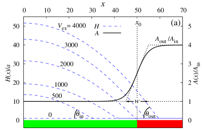
Figure 3: (a) Stationary cross section profiles of the liquid ridge on a chemical channel of half width $x_{0}=50$ and with edges of effective width $w=10$ for excess cross-sections $V_{\text{ex}}=$ 0, 500, 1000, 2000, 3000, and 4000 [see Eq. (1)]. Also shown is the lateral dependence of the Hamaker constant $A$ in units or $A_{\mathrm{in}}$ and its main features as given by Eq. (6). $A/A_{\mathrm{in}}=1$ and $A/A_{\mathrm{in}}=A_{\mathrm{out}}/A_{\mathrm{in}}=4$ correspond to $\theta_{\text{in}}=\frac{\sqrt{3}}{2}\delta$ and $\theta_{\text{out}}=\sqrt{3}$$\delta$, respectively ($\delta=a/\lambda$ is the scale factor for the slopes, with the lateral scale $\lambda=a^{2}/\sqrt{\sigma/A_{\mathrm{in}}}$). (b) $\left(P,V_{\text{ex}}\right)$ for the same values of $A_{\text{in}}$ and $A_{\text{out}}$ as in (a) for $w=10$ (dashed line, with dots indicating those systems which the profiles in (a) correspond to), $20$ (dash-dotted line), and $30$ (solid line) . The thinner lines correspond to the power laws $P\propto V_{\mathrm{ex}}^{-1/2}$ given by Eqs. (5) and (15) for ridges resting on homogeneous substrates corresponding to the outside of the channel (dash-double-dotted) and to the inside of the channel (dotted). For $w\gtrsim 30$ , $P(V_{\text{ex}})$ is monotonic while for $w\lesssim 30$ there is a range of cross-sections for which $\frac{\mathrm{d}P}{\mathrm{d}V_{\text{ex}}}>0$.

First, we analyze the pressure $P$ as a function of the excess cross-section $V_{\text{ex}}$ [see Eq. (1)] and how it is affected by the chemical heterogeneity of the substrate [see Fig. 3(b)]. Each point $\left(V_{\text{ex}},P\right)$ corresponds to a liquid ridge [Fig. 3(a)] centered around the axis of the chemical channel. The outer part of the substrate is covered by a film of thickness close to $1$, which is governed by the disjoining pressure. In the central region of the ridge, the thickness is large so that due to the vanishing of $\Pi$ for large $H$ the profile is determined by the capillary term $H^{\prime\prime}(x)$ in Eq. (11). The edges of the liquid ridge can be located inside the channel (i.e., at $\left|x\right|<x_{0}$), be “pinned” at the chemical steps (i.e., at $\left|\left|x\right|-x_{0}\right|\leq w$), or “spill” onto the surrounding substrate (i.e., at $\left|x\right|>x_{0}$). In that latter case, the channel will have little effect on the system, and a spilling ridge has properties similar to those of a ridge on a homogeneous substrate without a chemical channel.

The major features of the $\left(V_{\mathrm{ex}},P\right)$ diagram in Fig. 3(b) are the following. If the edge of a large ridge (i.e., apex height $\gg 1$) is well inside or well outside the channel, $P(V_{\mathrm{ex}})$ exhibits a power law $P\propto V_{\mathrm{ex}}^{-1/2}$ with a prefactor which increases with the equilibrium contact angle $\bar{\theta}_{\mathrm{eq}}$ . In the semi-macroscopic limit the prefactor is given by Eqs. (5) and, c.f., (15). For edges pinned at sufficiently sharp chemical steps (i.e., for sufficiently small $w$) the crossover between the power laws corresponding to the inner and outer parts of the channel features a change of sign for the slope $\frac{\mathrm{d}P}{\mathrm{d}V_{\mathrm{ex}}}$. The latter feature is important for the main focus of our study, because $\frac{\mathrm{d}P}{\mathrm{d}V_{\mathrm{ex}}}>0$ will turn out as the criterion of ridge stability.

In the following we first analyze a ridge on a homogeneous substrate, governed by capillarity and resting on a film the thickness of which is determined by the effective interface potential. From these semi-macroscopic considerations we derive the power law $P\propto V_{\mathrm{ex}}^{-1/2}$ and discuss features and limitations of the semi-macroscopic model which will be relevant for the pearling instability to be discussed in Sec. V.

Assuming that the expression for $P$ in Eq. (7c) reduces to $-\mathbf{\nabla}^{2}H$ for the ridge, and to $-\Pi$ for the wetting film, we obtain, for a homogeneous substrate, the following simple shape for a ridge of half-width $r$:

$$H(x)=\left\{\begin{array}[]{ccl}H_{\mathrm{film}}+\frac{P}{2}\left(r^{2}-x^{2}\right)&\text{if}&\left|x\right|<r\,,\\ H_{\mathrm{film}}&\text{if}&r<\left|x\right|\,.\end{array}\right.$$ (12)

The wetting film thickness $H_{\mathrm{film}}=1+P/\left(8\bar{\theta}_{\mathrm{eq}}^{2}\right)$ is obtained by solving $-\Pi(H_{\mathrm{film}})=P$ for $H_{\mathrm{film}}\approx 1$ and $P\ll 1$. The half-width $r$ is determined by the contact angle according to $\tan(\bar{\theta})=\left|\frac{\partial H}{\partial x}(x=r)\right|\delta$ so that $\bar{\theta}=\theta/\delta\simeq P\,r$. The contact angle $\bar{\theta}$ of the ridge depends on the pressure $P$ via $H_{\mathrm{film}}$:

$$\bar{\theta}=\frac{1}{\delta}\arccos\left[1+\Phi(H_{\mathrm{film}})/\sigma\right]\,.$$ (13)

However, to leading order in $P$ this is simply the equilibrium contact angle $\bar{\theta}_{\mathrm{eq}}=\frac{1}{\delta}\arccos\left[1+\Phi(a)/\sigma\right]$ given by Eq. (5) and the first correction is quadratic in $P$.

In order to justify the auxiliary role of the thin film despite the intrinsic lateral finite-size effect (see Sec. II), we investigate that regime in which the macroscopic characteristics of $H(x)$ dominate. For the shape given by Eq. (12) and with $P=\bar{\theta}/r$ one obtains for the cross-section $V=\int_{-L}^{L}H(x)\mathrm{d}x$ and the excess cross-section $V_{\mathrm{ex}}$ the following expressions:

$$V-V_{\mathrm{ex}}=2\,L\,\left(1+\frac{P}{8\,\bar{\theta}^{2}}\right)=2\,L\,\left(1+\frac{1}{8\,\bar{\theta}\,r}\right)$$ (14)

and

$$V_{\mathrm{ex}}=\frac{2}{3}Pr^{3}=\frac{2}{3}\bar{\theta}r^{2}=\frac{2}{3}\bar{\theta}^{3}/P^{2}.$$ (15)

Equation (15) implies that for fixed $\bar{\theta}$ one has $P\propto V_{\mathrm{ex}}^{-1/2}$. In order to ensure that the film at $x=\pm L$ is indeed flat, one has to choose the system size $L$ much larger than the ridge width $2\,r$, i.e., $L\gg r$. Moreover, the scaled thickness of the film outside the ridge should be close to its equilibrium value $1$, which requires $r\,\bar{\theta}\gg 1/8$, independently of $L$. As long as these two criteria are satisfied, the excess cross-section $V_{\mathrm{ex}}$ will be, by construction, independent of the system size $2\,L$.

As we shall show in Sec. V, $\frac{\mathrm{d}P}{\mathrm{d}V}$ and $\int Q\,\mathrm{d}x$ are two key quantities which determine the stability of the liquid ridge. To a good approximation both should be independent of the system size.

For the pressure $P$ this means that the derivative with respect to the total cross-section $V$ should be approximately equal to the derivative with respect to the excess cross-section $V_{\mathrm{ex}}$. From Eqs. (14) and (15) one obtains the ratio of the derivatives with respect to $V_{\mathrm{ex}}$ and $V$:

$$\frac{\mathrm{d}P}{\mathrm{d}V_{\mathrm{ex}}}\,\left(\frac{\mathrm{d}P}{\mathrm{d}V}\right)^{-1}=\frac{\mathrm{d}V}{\mathrm{d}V_{\mathrm{ex}}}\\ =1+2L\frac{\mathrm{d}}{\mathrm{d}V_{\mathrm{ex}}}\left(\frac{P}{8\bar{\theta}^{2}}\right)=1-\frac{3\,L}{16\,\bar{\theta}^{2}\,r^{3}},$$ (16)

where the substrate characteristics $L$ and $\bar{\theta}$ are kept constant. This poses an upper bound on the system size: $3\,L\ll 16\,\bar{\theta}^{2}\,r^{3}$, which quantifies the lateral finite-size effect outlined in Sec. II: if the width $2\,r$ of a ridge is small enough with respect to the total system size $2L$, the surrounding film can drain liquid from the ridge while acquiring less additional pressure than the shrunk ridge. This basic instability of stationary ridges (or drops) on arbitrarily large substrates is a consequence of the smoothly varying effective interface potential $\Phi$.

For the shape given in Eq. (12) one can also calculate the integral over $x$ of the mobility factor $Q(H)=\frac{H^{3}}{3}$. For sufficiently large ridges (such that $P$ is small and thus the film thickness is close to $1$, i.e., $r\,\bar{\theta}\gg 1/8$) one obtains

$$\int\limits_{-L}^{L}Q\left[H(x)\right]\,\mathrm{d}x=\frac{2\,L}{3}+\frac{2}{3}\,\bar{\theta}r^{2}+\frac{4}{15}\,\bar{\theta}^{2}r^{3}+\frac{4}{105}\bar{\theta}^{3}r^{4}.$$ (17)

The last term on the right-hand side is the excess mobility integral which can be written in terms of $V_{\mathrm{ex}}=\frac{2}{3}\bar{\theta}r^{2}$ as

$$\left[\int Q\mathrm{d}x\right]_{\text{ex}}=\int\limits_{-L}^{L}Q\left[H(x)-H_{\mathrm{film}}\right]\,\mathrm{d}x=\frac{3\,\bar{\theta}}{35}V_{\mathrm{ex}}^{2}.$$ (18)

The second and the third term on the right hand side of Eq. (17) are negligible: the respective ratios with the excess mobility integral are $\propto(\bar{\theta}\,r)^{-2}$ and $\propto(\bar{\theta}\,r)^{-1}$, respectively, and hence small in the limit of large $r$ considered here (see above). For $\bar{\theta}^{3}r^{4}\gg\frac{35}{2}L$ the excess mobility integral dominates the contribution from the film. A similar argument can be formulated in the presence of slippage at the substrate, i.e., for a more general expression of $Q$.

The lower bound on $L$ is thus $\propto r$ (so that the liquid ridge does not interfere with its periodic images), while the upper bounds are $\propto r^{3}$ [see the text after Eq. (16)] and $\propto r^{4}$ (see above). This implies that for every large enough $r$ one can find a range of system sizes $L$ within which the key quantities of the linear stability (as discussed in the following section) are independent of $L$ and of the macroscopic ridge cross-section $V_{\mathrm{ex}}$.

V Linear stability analysis

In order to assess the stability of a liquid ridge on a chemical channel, we consider the time evolution of small perturbations of the stationary film thickness as well as the corresponding small perturbations of the pressure and the flows. Since the base state is translationally invariant in the $y$ direction, we consider perturbations with the form of plane waves:

$$\widetilde{H}(x,y,t) = H(x)+\varepsilon\,h(x)\,e^{\omega\,t-i\,k\,y},$$ (19a)

$$\widetilde{P}(x,y,t) = P+\varepsilon\,p(x)\,e^{\omega\,t-i\,k\,y},$$ (19b)

$$\widetilde{J}_{x}(x,y,t) = 0+\varepsilon\,j_{x}(x)\,e^{\omega\,t-i\,k\,y},$$ (19c)

$$\widetilde{J}_{y}(x,y,t) = J_{y}(x)+\varepsilon\,j_{y}(x)\,e^{\omega\,t-i\,k\,y},$$ (19d)

with $\varepsilon\ll 1$ . Insertion into Eqs. (7a-c) and expansion to first order in $\varepsilon$ leads to the following linear eigenvalue problem for the complex growth rate $\omega(k)$:

$$\omega(k)\,h = -\frac{\mathrm{d}j_{x}}{\mathrm{d}x}-k^{2}\,Q\,p+i\,k\,g\,\left.\frac{\mathrm{d}Q}{\mathrm{d}\widetilde{H}}\right|_{H}h\,,$$ (20a)

$$j_{x} = -Q\,\frac{\mathrm{d}p}{\mathrm{d}x}\,,$$ (20b)

$$p = \left(k^{2}-\left.\frac{\partial\Pi}{\partial\widetilde{H}}\right|_{H}\right)\,h-\frac{\mathrm{d}h^{\prime}}{\mathrm{d}x}\,,$$ (20c)

$$h^{\prime} = \frac{\mathrm{d}h}{\mathrm{d}x}\,.$$ (20d)

In order to solve this problem numerically by continuation from a simple configuration, one must integrate Eq. (11) for the stationary profile and the linearized equations (20) together. As in Sec. (IV), we render the system autonomous by introducing $s=\frac{x}{L}$ and converting $x$ into a component of the solution vector. This leads to the following first-order system of non-linear equations:

$$\frac{\mathrm{d}}{\mathrm{d}s}\left(\begin{array}[]{c}x\\ H\\ H^{\prime}\\ h\\ h^{\prime}\\ p\\ j_{x}\end{array}\right)=L\,\left(\begin{array}[]{c}1\\ H^{\prime}\\ -\Pi-P\\ h^{\prime}\\ \left(k^{2}-\frac{\partial\Pi}{\partial H}\right)h-p\\ -j_{x}/Q\\ -\left(\omega-ikg\frac{\mathrm{d}Q}{\mathrm{d}H}\right)h-k^{2}Qp\end{array}\right).$$ (21)

We note that $h$, $h^{\prime}$, $p$, and $j_{x}$ are in general complex valued functions of $s$. Only for $g=0$ there are real solutions.

The spectrum is semi-discrete. The wavevector $k$ along the $y$ direction is continuous, while the solutions of Eq. (21) for a given $k$ are generated by a discrete family of modes due to the finite lateral extent $L$. We are primarily interested in the varicose or pearling mode, which is obtained by continuation from the fundamental symmetric mode, which in the simple case of a homogeneous substrate covered by a film of thickness $H=1$ corresponds to perturbations in the $y$ direction only:

$$h = 1\,,$$ (22)

$$j_{x} = 0\,,$$ (23)

$$p = k^{2}+6A\,,$$ (24)

$$\omega(k) = ikg-k^{2}\left(k^{2}+6A\right)\,.$$ (25)

Since $A=\frac{4}{3}\,\bar{\theta}^{2}>0$, $\mathrm{Re}\,\omega=-k^{2}\left(k^{2}+6A\right)<0$ and for any $k\neq 0$ the fundamental symmetric mode is unconditionally stable on a homogeneous substrate covered by a flat residual film. It is only in homogeneous situations that this mode (i.e., a plane wave along the $y$-direction) has no nodes along the $x$-direction [see, c.f., Eq. (30)].

V.1 Systems without drive: $g=0$

The Rayleigh-Plateau instability occurs for long wavelengths, i.e., $k\rightarrow 0$. For large $k$, however, surface tension will stabilize all perturbations and we expect $\omega(k)\sim-k^{4}$ in this limit. In order to assess the stability of a liquid ridge, we therefore focus on the limit $k\to 0$. Since the mode with $k=0$ is marginally stable due to volume conservation, we have to infer the stability or instability of a ridge from the eigenvalue for small nonzero values of $k$.

Figure 4: Part (a) shows the $\left(P,V_{\text{ex}}\right)$ diagram of the stationary solutions for a given substrate heterogeneity ($A_{\text{in}}=1$, $A_{\text{out}}=4$, $w=10$, $x_{0}=50$; compare Fig. 3). In this case the chemical steps are sharp enough for a change of sign of $\frac{\mathrm{d}P}{\mathrm{d}V_{\text{ex}}}$ in a finite interval of excess cross sections $V_{\mathrm{ex}}$. As function of $V_{\mathrm{ex}}$ part (b) shows the growth rate $\mathrm{Re}\,\omega(k;V_{\text{ex}})$ [divided by $k^{2}$ and multiplied by $P(V_{\text{ex}})$] of long-wavelength varicose modes for several small values of $k$. The stability window of the varicose mode corresponds to the range where $\frac{\mathrm{d}P}{\mathrm{d}V_{\text{ex}}}>0$. Note that for small wave numbers $k$ and large $V_{\text{ex}}$, $P\,\omega(V_{\text{ex}},k)/k^{2}$ approaches a plateau [with a value predicted by Eq. (35) to be $\frac{9}{35}=0.26$; for large $V_{\mathrm{ex}}$ one has $\bar{\theta}_{\mathrm{eq}}^{2}=3A_{\mathrm{out}}/4=3$, which is consistent with the observed value]. On the present scales the curves for $k\lesssim 10^{-3}$ would be barely distinguishable from the one for $k=10^{-3}$. For $k=0.01$ a typical stabilization can be seen for $V_{\mathrm{ex}}\gtrsim 17000$, as the wavelength corresponding to $k$ becomes short with respect to the ridge width. For $k=0.1$ a finite-size effect is observed for $V_{\mathrm{ex}}\gtrsim 2500$: in this case the mode does no longer correspond to a bulging of the ridge but to system-wide perturbations of the film, which are stable.

Figure 4 shows the pressure $P$ for a chemical channel with $w=10$ [compare Fig. 3(b)] and the (purely real) growth rate $\omega$ of long-wavelength perturbations [determined numerically by solving Eq. (21)] as a function of the excess cross-section $V_{\mathrm{ex}}$. We emphasize two features of this figure.

First, the juxtaposition of the two graphs clearly suggests $\frac{\mathrm{d}P}{\mathrm{d}V_{\mathrm{ex}}}>0$ as a stability criterion for large-wavelength deformations of the ridge. All long-wavelength modes possess a stability domain [$\omega(k;V_{\text{ex}})<0$], which includes the range of $V_{\mathrm{ex}}$ for which $\frac{\mathrm{d}P}{\mathrm{d}V_{\mathrm{ex}}}>0$. These are also the cross-sections for which the edges of the ridge are pinned at the channel edge (see Fig. 3).

Second, for values of $V_{\mathrm{ex}}$ for which the edges of the base state of the liquid ridge are well outside the chemical channel, $\omega(V_{\mathrm{ex}},k)\,P(V_{\mathrm{ex}})/k^{2}$ converges to a constant independent of $V_{\mathrm{ex}}$ for $k\to 0$. This is characteristic for ridges resting on homogeneous substrates, and we shall derive a corresponding analytic expression below.

The first observation has a simple explanation. A long wavelength perturbation corresponds to a periodic arrangement of liquid bumps separated by thinned regions. For small $k$, the transition regions between the bumps and the thinned regions can be ignored and the pressure in such a bump is approximately given by the pressure in a homogeneous ridge of corresponding cross section. If $\frac{\mathrm{d}P}{\mathrm{d}V}>0$, the pressure in the thicker part will be larger than in the thinner part and the liquid will flow from the bump to the thin part, leveling the perturbation. If, on the other hand, $\frac{\mathrm{d}P}{\mathrm{d}V}<0$, the pressure in the bump will be smaller than in the thin part, the bump will be inflated (for the same reason as a small soap bubble inflates a larger one), and the perturbation will grow.

In the following we shall confirm the phenomenological stability criterion $\frac{\mathrm{d}P}{\mathrm{d}V}>0$ by a perturbation analysis for small $k$ of the eigenvalue problem formulated in Eq. (20). To this end, for $g=0$ we write Eq. (20) as a differential equation of fourth order for $h(x;k)$:

$$\omega(k)\,h(x;k)=\left(\hat{F}+\hat{K}\right)\,h(x;k)$$ (26)

with the $k$-independent linear operator

$$\hat{F}=-\frac{\partial}{\partial x}Q(H)\frac{\partial}{\partial x}\left(\frac{\partial\Pi}{\partial H}+\frac{\partial^{2}}{\partial x^{2}}\right)$$ (27)

and the $k$-dependent linear operator

$$\hat{K}=k^{2}\,Q(H)\,\left(\frac{\partial\Pi}{\partial H}+\frac{\partial}{\partial x^{2}}-k^{2}\right)+k^{2}\frac{\partial}{\partial x}\left[Q(H)\frac{\partial}{\partial x}\right].$$ (28)

Both $\hat{F}$ and $\hat{K}$ act on $h(x;k)$ via multiplication followed by $\frac{\partial}{\partial x}$. With the usual scalar product $\langle\phi|\psi\rangle=\frac{1}{2\,L}\int_{-L}^{L}\bar{\phi}(x)\,\psi(x)\,\mathrm{d}x$ in the space of $2\,L$-periodic complex valued functions, where the overbar indicates complex conjugation, the adjoint operator to $\hat{F}$ is

$$\hat{F}^{\dagger}=-\left(\frac{\partial\Pi}{\partial H}+\frac{\partial^{2}}{\partial x^{2}}\right)\,\frac{\partial}{\partial x}\left[Q(H)\frac{\partial}{\partial x}\right]\,.$$ (29)

By construction, $\hat{F}$ and $\hat{F}^{\dagger}$ have the same discrete spectrum of eigenvalues $\omega_{n}(k=0)$ and the eigenfunctions $f_{n}(x)$ (of $\hat{F}$) and $f_{n}^{*}(x)$ (of $\hat{F}^{\dagger}$, also called left eigenfunctions of $\hat{F}$) to different eigenvalues are orthogonal, i.e., $\langle f_{n}^{*}|f_{m}\rangle=\delta_{nm}$. (Recall that $\bar{f}_{n}$, not $f_{n}^{*}$, is the complex conjugate to $f_{n}$.) Since both operators commute with the parity operator, in the following we can restrict our analysis to modes symmetric with respect to $x=0$. As we already observed for the numerical solution, the mode relevant for the pearling instability is the fundamental symmetric mode. By differentiating Eq. (11) with respect to $P$ one can show that $\frac{\mathrm{d}H}{\mathrm{d}P}(x)=\frac{\mathrm{d}H}{\mathrm{d}V}(x)/\frac{\mathrm{d}P}{\mathrm{d}V}$ is an eigenfunction of $\hat{F}$ corresponding to the eigenvalue $\omega_{0}(k=0)=0$. The normalized set of fundamental modes is then

$$f_{0}(x)=2\,L\,\frac{\mathrm{d}H(x)}{\mathrm{d}V}\quad\text{and}\quad f_{0}^{*}(x)=1\,.$$ (30)

Although $f_{0}(x)$ is the fundamental mode, in the interval $[0,L]$ it can have a (single) zero at the edge of the ridge. On the ridge $\frac{\mathrm{d}H(x)}{\mathrm{d}V}$ is positive, whereas on the surrounding flat film it is negative if $\frac{\mathrm{d}P}{\mathrm{d}V}<0$. One can show that $\langle f_{0}^{*}|f_{0}\rangle=1$ by swapping the integration with respect to $x$ and the differentiation with respect to $V$. The model shape given by Eq. (12), where $H_{\mathrm{film}}=1+P/\left(8\,\bar{\theta}_{\mathrm{eq}}^{2}\right)$, provides an instructive illustration.

For small $k$, we assume that the fundamental eigenmode $h_{0}\left(x;k\right)$ differs only slightly from $f_{0}(x)$ and we can expand it (up to a normalization constant which we do not need to consider) in terms of eigenfunctions of $\hat{F}$:

$$h_{0}(x;k)=f_{0}(x)+\sum\limits_{n>0}a_{n}(k)\,f_{n}(x)\,,$$ (31)

with expansion coefficients $a_{n}(k)$ of order $k$. One obtains the lowest order correction to $\omega_{0}(k)$ by inserting $h_{0}(x;k)$ from Eq. (31) into Eq. (26) and projecting the result onto $f_{0}^{*}$, keeping only terms up to order $k^{2}$. With $\langle f_{0}^{*}|f_{0}\rangle=1$ one finds

$$\omega_{0}(k)=\omega_{0}(0)+k^{2}\,\left\langle f_{0}^{*}\left|Q(H)\left(\frac{\partial\Pi}{\partial H}+\frac{\partial^{2}}{\partial x^{2}}\right.\right)f_{0}\right\rangle\\ +k^{2}\,\left\langle f_{0}^{*}\left|\frac{\partial}{\partial x}\left[Q(H)\frac{\partial}{\partial x}f_{0}\right]\right.\right\rangle.$$ (32)

The nature of $f_{0}$ implies $\omega_{0}(0)=0$ as detailed previously. The integrand in the scalar product in the last term is a total derivative so that for a $2\,L$-periodic function this term vanishes. For the first scalar product on the right hand side the integrand reduces to $Q(H)\,\frac{\mathrm{d}P}{\mathrm{d}V}$ which implies

$$\omega_{0}(k)=-k^{2}\,\frac{\mathrm{d}P}{\mathrm{d}V}\,\int\limits_{-L}^{L}Q\left[H(x)\right]\,\mathrm{d}x\,.$$ (33)

We note that Eq. (33) is valid for a general expression of the mobility factor $Q(H)$, not only for the no-slip case studied numerically. In general the velocity field is such that $Q(H)>0$, so that the integral in Eq. (33) is positive. This confirms the observation made for the numerical solution and supports the heuristic argument given at the beginning of this subsection, i.e., that the stationary ridge is stable for $\frac{\mathrm{d}P}{\mathrm{d}V}>0$. A similar discussion can be carried out for a more general mobility factor which could depend explicitly on $x$.

For the macroscopic ridge described by Eq. (12) one has $\frac{\mathrm{d}P}{\mathrm{d}V}\approx\frac{\mathrm{d}P}{\mathrm{d}V_{\mathrm{ex}}}=\frac{\mathrm{d}P}{\mathrm{d}r}/\frac{\mathrm{d}V_{\mathrm{ex}}}{\mathrm{d}r}$. The generalization of Eq. (15) to heterogeneous substrates by introducing an effective local contact angle $\bar{\theta}_{\mathrm{eq}}(x)$ leads, at the ridge edge ($x=r$), to $P=\bar{\theta}_{\mathrm{eq}}(r)/r$ and $V_{\mathrm{ex}}=\frac{2}{3}\,r^{2}\,\bar{\theta}_{\mathrm{eq}}(r)$. Since the equilibrium contact angle inside the channel is smaller than outside one has $\mathrm{d}\bar{\theta}_{\mathrm{eq}}(r)/\mathrm{d}r>0$ and therefore $\mathrm{d}V_{\mathrm{ex}}/\mathrm{d}r>0$. However, the pressure as a function of the half ridge width $r$ can be nonmonotonous. From $\frac{\mathrm{d}P}{\mathrm{d}r}=\left[\mathrm{d}\bar{\theta}_{\mathrm{eq}}(r)/\mathrm{d}r-\bar{\theta}_{\mathrm{eq}}(r)/r\right]/r$ one obtains as a macroscopic stability criterion

$$\frac{1}{\bar{\theta}_{\mathrm{eq}}(r)}\,\frac{\mathrm{d}\bar{\theta}_{\mathrm{eq}}(r)}{\mathrm{d}r}=\frac{\mathrm{d}\ln\bar{\theta}_{\mathrm{eq}}(r)}{\mathrm{d}r}>\frac{1}{r}.$$ (34)

For a homogeneous substrate $\omega_{0}(k)$ can be determined in the macroscopic limit discussed in Sec. IV. For a given contact angle $\bar{\theta}_{\mathrm{eq}}$ Eqs. (15) and (18) yield

$$\omega_{0}(k)=k^{2}\,\frac{1}{7}\sqrt{\frac{3\,\bar{\theta}_{\mathrm{eq}}^{5}}{2}}\,\sqrt{V_{\text{ex}}}=k^{2}\,\frac{\bar{\theta}_{\mathrm{eq}}^{4}}{35}\,\frac{1}{P}$$ (35)

as a function of $V_{\text{ex}}$ or $P$, respectively. These relations provide an understanding for the numerical observation in Fig. 4 that for small $k$ the growth rate rescaled by $k^{2}/P$ approaches a constant as $V_{\mathrm{ex}}\to\infty$, i.e., in the limit of a homogeneous substrate.

V.2 Systems with drive: $g\neq 0$

Figure 5: For reference purposes part (a) corresponds to the rotated Fig. 4(b), obtained for the case without drive, with the curve for $k=0.1$ removed. Part (b) traces the two zeros of $\text{Re}\,\,\omega(k)$ as a function of the drive $g$ by showing the isolines of $\text{Re}\,\,\omega(k;V_{\text{ex}},g)=0$ for selected small values of $k$. Ridges with cross-sections between the horizontal lines are stable. Other ridges are unstable with respect to pearling, with the marginally stable wavelength depending on the drive. The channel parameters are the same as in Fig. 4.

Figure 6: (a) Curve of marginal stability, $\text{Re}\,\,\omega(k;g,V_{\text{ex}})=0$, in the $g$-$k$-plane (full line) for $V_{\text{ex}}=10^{4}$ (i.e., outside the stability region for $g=0$, see Fig. 5) and the same channel parameters as in Figs. 4 and 5. For large $g$, the drive required to stabilize modes with large wavelengths is proportional to $1/k$. The straight dashed line is a fit $k\propto 1/g$ to the curve for $g>10^{3}$. (b) The growth rate $\text{Re}\,\,\omega(k;g,V_{\text{ex}})$ as function of $g\,k$ for the same ridge and several values $g$. For large $g$ the curves approach a limiting curve $\omega_{\infty}(g\,k;V_{\text{ex}})$, which depends on $g$ and $k$ only via the product $g\,k$.

Figure 5(b) shows the isolines $\text{Re}\,\,\omega(k;g,V_{\text{ex}})=0$ in the $g$-$V_{\text{ex}}$-plane for several values of $k$. For $g=0$, the corresponding values of $V_{\mathrm{ex}}$ are the zeros of the curves in Fig. 4(b), repeated for convenience in Fig. 5(a). For small values of $k>0$, as function of $g$ the isolines follow the two horizontal lines, which mark the lower and upper cross-sections for which $\frac{\mathrm{d}P}{\mathrm{d}V_{\text{ex}}}=0$, up to larger values of $g$ before they turn away from these lines. However, they never penetrate the range of cross-sections between the two horizontal lines. Thus ridges in this range of excess cross-sections remain stable also under drive. For ridges with $V_{\mathrm{ex}}$ outside of this range Fig. 5(b) leads to the following conjectures. For any $V_{\mathrm{ex}}$, modes with a given $k$ are stabilized by a large enough drive $g>g_{c}(k,V_{\mathrm{ex}})$ (see below). On the other hand, for every ridge and every finite value of $g$ there is a sufficiently small wave number $k_{c}(g,V_{\mathrm{ex}})$ such that modes with smaller wave numbers $k<k_{c}(g,V_{\mathrm{ex}})$ are unstable. Therefore drive cannot stabilize a liquid ridge versus pearling as such, but it shifts the critical wavelength for the onset of instability to larger values. Hence with driven flow we expect the appearance of larger pearls which also emerge further apart from each other.

For $g\neq 0$ one needs the full eigenvalue spectrum $\omega_{n}(k)$, for all $n\geq 0$, in order to compute the lowest order correction to $\omega_{0}(0)$ for small $k$ in the perturbation analysis presented in Subsec. V.1. However, for large $g$ and small $k$ we expect that the last term in Eq. (20a), i.e., the term proportional to $g$, dominates the eigenvalue problem, which turns $\omega(k,g)$ into a function of $g\,k$. We have confirmed this expectation numerically. Figure 6(a) shows the stability boundary for a given ridge cross-section $V_{\mathrm{ex}}$ in the $g$-$k$-plane. For large $g$ the critical wave number $k_{c}(g,V_{\mathrm{ex}})$, for which $\mathrm{Re}\,\omega\left[k_{c}(g,V_{\mathrm{ex}});g,V_{\mathrm{ex}}\right]=0$, is indeed proportional to $1/g$ . Modes with smaller $k$ (or longer wavelength) require a larger drive to be stabilized. However, for every drive $g$ there are unstable modes. For a given cross-section $V_{\mathrm{ex}}$ and increasing values of $g$ Fig. 6(b) shows the growth rate $\mathrm{Re}\,\omega(k;g,V_{\mathrm{ex}})$ as a function of $g\,k$ for increasing values of $g$. As expected the curves converge to a limiting curve $\omega_{\infty}(g\,k;V_{\mathrm{ex}})$. Interestingly, $\omega_{\infty}(g\,k;V_{\mathrm{ex}})\sim(g\,k)^{2}$ for large as well as for small values of $g\,k$, but with different prefactors (positive for $gk\lesssim 10^{-10}$, negative for $gk\gtrsim 10^{-9}$).

VI Summary and conclusions

As illustrated in Fig. 1, we have used the lubrication approximation in order to analyze the stability of nonvolatile liquid ridges versus pearling in the case of driven flow along a chemical stripe with smooth edges (see Fig. 2). Such ridges can be stable versus pearling even though their contact lines are not completely pinned (see Fig. 3). In an analytic perturbation analysis for small wave numbers $k$ as well as numerically (see Fig. 4) we have confirmed $\frac{\mathrm{d}P}{\mathrm{d}V}>0$ as the corresponding stability criterion, i.e., a ridge is stable versus pearling if the pressure $P$ in the ridge increases with its cross-section $V$. If the ridge is guided by a chemical channel with smooth edges, which can be characterized by a laterally varying effective contact angle $\theta_{\mathrm{eq}}(x)$, we find the stability criterion $\frac{\mathrm{d}\ln\theta_{\mathrm{eq}}(x)}{\mathrm{d}x}>\frac{1}{x}$ where $x$ is the lateral distance from the center of the stripe. This criterion for the chemical design of the stripe also holds if a body force aligned with the channel drives the liquid.

We find a stabilizing effect of drive (see Fig. 5). Stable modes remain stable under drive but the critical wavenumbers $k_{c}$ (such that modes with $k<k_{c}$ are unstable) decrease with drive. Therefore, whenever the ridge is indeed subject to the pearling instability, we expect the size of the emerging pearls and the distance between them to increase with drive. For any finite drive, there is a nonzero range of long wavelengths for which the modes are unstable. Hence the pearling instability cannot be suppressed by flow. These findings are in agreement with the results in Ref. koplik06a for well-filled ridges with large contact angles $\geq 90^{\circ}$ and a fixed contact line. However, in contrast to the case of well-filled ridges, in the thin film limit the maximum of the growth rate $\text{Re}\,\,\omega$ of unstable modes does not increase with drive (see Fig. 6).

We thank M. Brinkmann for fruitful discussions. M. Rauscher acknowledges financial support from the priority program SPP 1164 “Micro and Nano Fluidics” of the Deutsche Forschungsgemeinschaft under grant number RA 1061/2-1.

References

- (1) N. Giordano and J.-T. Cheng, J. Phys.: Condens. Matter 13, R271 (2001).
- (2) P. Mitchell, Nature Biotech. 19, 717 (2001).
- (3) H. A. Stone and S. Kim, AIChE J. 47, 1250 (2001).
- (4) A. A. Darhuber, S. M. Troian, and W. W. Reisner, Phys. Rev. E 64, 031603 (2001).
- (5) S. Dietrich, M. N. Popescu, and M. Rauscher, J. Phys.: Condens. Matter 17, S577 (2005).
- (6) H. Gau, S. Herminghaus, P. Lenz, and R. Lipowsky, Science 283, 46 (1999).
- (7) B. Zhao, J. S. Moore, and D. J. Beebe, Anal. Chem. 74, 4259 (2002).
- (8) M. Brinkmann, J. Kierfeld, and R. Lipowsky, J. Phys.: Condens. Matter 17, 2349 (2005).
- (9) M. Brinkmann and R. Lipowsky, J. Appl. Phys. 92, 4296 (2002).
- (10) S. Mechkov, G. Oshanin, M. Rauscher, M. Brinkmann, A. M. Cazabat, and S. Dietrich, Europhysics Lett., 80, 66002 (2007).
- (11) M. Brinkmann, J. Kierfeld, and R. Lipowsky, J. Phys. A: Math. Gen. 37, 11547 (2004).
- (12) S. H. Davis, J. Fluid Mech. 98, 225 (1980).
- (13) J. Koplik, T. S. Lo, M. Rauscher, and S. Dietrich, Phys. Fluids 18, 032104 (2006).
- (14) J. R. King, A. Münch, and B. Wagner, Nonlinearity 19, 2813 (2006).
- (15) C. Bauer, S. Dietrich, and A. O. Parry, Europhysics Lett. 47, 474 (1999).
- (16) A. Oron, S. H. Davis, and S. G. Bankoff, Rev. Mod. Phys. 69, 931 (1997).
- (17) Auto is a publicly available software for continuation and bifurcation problems in ordinary differential equations originally written in 1980 and widely used in the dynamical systems community. Project homepage: http://sourceforge.net/projects/auto2000/
- (18) P. G. de Gennes, Rev. Mod. Phys. 57, 827 (1985).
- (19) S. Dietrich, in Phase Transitions and Critical Phenomena, edited by C. Domb and. J. L. Lebowitz, (Academic, London, 1988), Vol. 12, p. 1.
- (20) S. Dietrich and M. Napiórkowski, Phys. Rev. A 43, 1861 (1991).
- (21) J. S. Langer, Rev. Mod. Phys. 52, 1 (1980).
- (22) In practice, the velocity profile is affected by the heterogeneous chemical properties of the substrate, in particular via the Navier slip length. This would lead to an explicit dependence of the mobility factor on the transverse coordinate . However, in our study we assume, unless mentioned otherwise, that the no-slip condition is fulfilled on the whole substrate, leading to the simple expression , which depends on only via . Some analytical results still hold for general and explicitly -dependent expressions for .
- (23) Here the picture of gravitational drive [Eq. (2b)] is used as an example, but the present study covers any kind of driving force acting on the bulk.