The corona and upper transition region of $\epsilon$ Eridani

Abstract

We present analyses of observations of $\epsilon$ Eridani (K2 V) made with the Low Energy Transmission Grating Spectrometer on Chandra and the Extreme Ultraviolet Explorer, supplemented by observations made with the Space Telescope Imaging Spectrograph, the Far Ultraviolet Spectroscopic Explorer and the Reflection Grating Spectrometer on XMM-Newton. The observed emission lines are used to find relative element abundances, to place limits on the electron densities and pressures and to determine the mean apparent emission measure distribution. As in the previous paper by simjordan03a, the mean emitting area as a function of the electron temperature is derived by comparisons with a theoretical emission measure distribution found from energy balance arguments. The final model has a coronal temperature of $3.4\times 10^{6}$ K, an electron pressure of $1.3\times 10^{16}$ cm${}^{-3}$K at $T_{\rm e}=2\times 10^{5}$ K and an area filling factor of 0.14 at $3.2\times 10^{5}$ K. We discuss a number of issues concerning the atomic data currently available. Our analyses are based mainly on the latest version of CHIANTI (v5.2). We conclude that the Ne/O relative abundance is 0.30, larger than that recommended from solar studies, and that there is no convincing evidence for enhanced coronal abundances of elements with low first ionization potentials.

1 Introduction

$\epsilon$ Eri (K2 V) is a nearby dwarf star that has been observed over a wide spectral range, from the infrared to X-ray wavelengths. Its fundamental parameters have been discussed by drakesmith93, where references to earlier work can be found, and more recently by difolco04 and ap04. difolco04 have derived the diameter of $\epsilon$  Eri from interferometric measurements and have also made models to check the self-consistency of their adopted parameters. A more recent measurement by difolco07 gives a radius that is smaller by only 0.008 $R_{\odot}$. The values of the parameters adopted here are given in Table 1 and are from difolco04, although these are also consistent with those found by drakesmith93, to within the combined uncertainties. Compared with the Sun, $\epsilon$ Eri has a shorter rotational period (11.68 d) (donahue96), a larger spatially averaged magnetic field (165 G) (rueedi97) and larger stellar surface emission line fluxes. It is, therefore, ideal for studies of a stellar outer atmosphere under conditions of higher mean magnetic activity than the Sun.

Observations with IRAS showed that $\epsilon$ Eri has an infrared excess, indicating the presence of dust; more recently a planet and a debris disk have been detected (hatzes00; greaves05). Further studies of the dust have been made by difolco07. Combining the above rotational period with $v\sin i=1.7$ km s${}^{-1}$ and $R_{*}=0.743R_{\odot}$ (difolco04), leads to $i=32^{\circ}$, similar to the value of 25${}^{\circ}$ suggested by greaves05 for the inclination of the debris disc to the plane of the sky.

Here we make use of observations at ultraviolet to X-ray wavelengths, as summarized in Table 2. In previous work we used observations with the Space Telescope Imaging Spectrograph (STIS) on the Hubble Space Telescope to identify forbidden lines of Fe xii (jordan01a) and to determine the electron pressure ($P_{\rm e}$) in the transition region (jordan01b). Including observations with the Far Ultraviolet Spectroscopic Explorer (FUSE), we have modelled the chromosphere and transition region, up to an electron temperature ($T_{\rm e}$) of $\simeq 3\times 10^{5}$ K (simjordan05).

Observations with the Extreme Ultraviolet Explorer (EUVE) have been analysed by a number of authors. schmitt96 used lines of iron to derive the emission measure distribution (EMD) at above $T_{\rm e}\simeq 6\times 10^{5}$ K and also placed limits on the electron density ($n_{\rm e}$) in the upper transition region from lines of Fe xiii and Fe xiv. laming96 used the same spectra to derive emission measures from lines of a range of elements and concluded that if any trends in abundances with the first ionization potential (FIP) were present, they were not significantly larger than in the solar corona. sf03 included further EUVE spectra and also derived the EMD. They found much larger values of $n_{\rm e}$ from lines of Fe xix and Fe xxi that are now superseded. simjordan03a used the line fluxes measured by schmitt96 to derive the EMD from the iron lines alone, adopting a more recent (smaller) value of the interstellar absorption by dring97 and using CHIANTI (v4) (dere97; young03) for line excitation atomic data. They compared the apparent EMD with that calculated from an energy balance in which the net thermal conductive flux was set equal to the local radiative energy loss and hence derived the fractional emitting area as a function of $T_{\rm e}$ ($\simeq 0.2$ at $2\times 10^{5}$ K).

High-resolution X-ray observations of $\epsilon$ Eri have been made with both the Low Energy Transmission Grating Spectrograph (LETGS) on Chandra and the Reflection Grating Spectrometer (RGS) on XMM-Newton. The former observations have been reduced and analysed by sf04 and wood06, who derived the EMD and relative element abundances, making use of the Astrophysical Plasma Emission Database (APED v1.3) (smith01) and CHIANTI (v4.2), respectively. Because there have been changes in the atomic data available, we have made our own analysis of the above spectra and the EUVE spectra, using CHIANTI (v5.2) (landi06). We have also made our own measurements of the X-ray line fluxes. $\epsilon$ Eri was included in a survey of stellar coronal densities by ness02, using LETGS spectra, and in a study of coronal opacities by ness03a, using LETGS and RGS spectra. Comparisons with these earlier results are made in later sections.

The first aim of the present work is to use all the available observations and up-to-date atomic data to derive the mean EMD, the relative element abundances and the electron densities and pressures. The mean EMD is then used in conjunction with new theoretical EMDs to refine the earlier values of the mean emitting areas.

Section 2 describes the X-ray observations used and the data reduction. Limits on $n_{\rm e}$ and $P_{\rm e}$ are discussed in Section 3, since these are required in deciding on the identification of some lines and in the analysis of some line fluxes. The identifications of particular lines are discussed in Section 4, in conjunction with the emission measures derived and some issues related to the atomic data. Section LABEL:S5 describes how the mean EMD and the relative element abundances were derived. In Section LABEL:S6, the theoretical EMD and the fractional areas occupied by the emitting regions are derived, using the method set out in simjordan03a. Our main conclusions are summarized in Section LABEL:S7.

Table 1: Stellar parameters adopted.

Distance${}^{a}$	Mass${}^{b}$	Radius${}^{b}$	$\log g_{*}^{b}$	$\log N_{\rm H}^{c}$
(pc)	($M_{\odot}$)	($R_{\odot}$)
3.218	$0.9\,\pm\,0.1$	$0.743\,\pm\,0.01$	$4.65\,\pm\,0.1$	$17.88\,\pm\,0.07$

${}^{a}$ The Hipparcos catalogue esa97.
${}^{b}$ difolco04; $g_{*}$ in cm s${}^{-2}$. ap04 give a value of $\log g_{*}=4.621$.
${}^{c}$ dring97; $N_{\rm H}$ in cm${}^{-2}$.

2 Observations and data reduction

2.1 X-ray observations

We use the Chandra LETGS spectra (ObsID 1869) that had an exposure time of 105.3 ks. We have also examined the spectra obtained with the XMM-Newton RGS instrument (ObsID 0112880501) that have an exposure time of 13 ks. These spectra are available from the Chandra and XMM-Newton archives.

The LETGS projects the dispersed spectrum onto a microchannel plate detector. The detector is placed behind the grating in a manner such that the non-dispersed photons (zeroth order) are recorded in the middle of the detector, with the two dispersion directions appearing as spectra in the plus and minus directions. There is overlap between the first-order spectra and the various higher-order spectra of shorter wavelengths and care must be taken to exclude higher order lines or to account for line blending when this occurs in important first-order lines. In the lists of lines given in Tables 3 and 4, purely higher-order lines are excluded and blends with first-order lines are noted.

2.2 Data reduction

We extracted the LETGS spectra on the plus and minus sides separately and calculated the effective areas using the standard CIAO tools (v3.2). The measurement of line fluxes was carried out with the CORA program developed by newi02. This accounts for the particular problems of low-count photon statistics (see, e.g., ness01). After trying several approaches we used a fixed line width (FWHM- Full width at half maximum) of 0.060 Å, since intrinsic stellar line widths are not resolvable.

As noted by others (see the extensive discussion in chung04), the apparent wavelengths of lines can differ between the plus and minus sides, leading to larger linewidths when the spectra in the plus and minus side spectra are summed. The line fluxes given in Tables 3 and about half of those in 4 are derived from the summed spectra, using variable line widths of between 0.053 and 0.080 Å, although the larger widths usually occur only at wavelengths above 90 Å. We have checked that these fluxes do not differ significantly from the averages of the fluxes in the individual plus and minus side spectra. Some lines are not observed, or are poorly observed, in one of the two spectra. In this case only one spectrum is used; the wavelengths of such lines are given in italic script in Table 4. We also give the effective areas adopted so that the original count rates can be recovered.

All the line fluxes have then been corrected for absorption in the interstellar medium (ISM) using a hydrogen column density of $\log N_{\rm H}$(cm${}^{-2}$) = 17.88 from dring97, lower than that used by sf03 who adopted a value of 18.1. The absorption model also includes He i, He ii and other abundant elements. Uncertainties in the line fluxes arise not only from the statistical measurement errors calculated by the CORA program, but also from the line widths adopted and the source continuum. The line widths in the LETGS spectra can be approximated by Moffat profiles (Lorentzians with an exponent $\beta$ = 2.4; drake04). The source continuum can be accounted for in CORA by adding a background (in counts s${}^{-1}$ Å${}^{-1}$) to the line templates. By varying the source background we found that in many cases, the dominant source of the uncertainty in line fluxes arises from the choice of the source background. The specific case of the lines of O vii is discussed in Section 3.

The APED (smith01) and CHIANTI (v5.2) (landi06) data bases were consulted in making the line identifications (see also Section 4). Lines marked with b are possibly blended but the identification of the main additional contributor is not certain and these lines are not used in the analyses of line fluxes. Blending between first-order lines occurs in several important cases. The methods used to find the relative contributions are discussed in Section 4. Fluxes were measured for all lines, but since our aim is to establish a reliable EMD a number of weak lines are not included in Tables 3 and 4, unless they have particular significance for our studies. A fuller list of lines present has been published by sf04.

There are systematic differences between laboratory and observed wavelengths above about 80 Å (where the observed wavelengths are too large), owing to the treatment of detector plate gaps (see chung04). Since we are not analyzing line shifts and are using only well identified lines in this region, we have not attempted to correct these wavelengths.

In reducing the RGS1 and RGS2 spectra we used Lorentzian line profiles to approximate the instrumental line profiles and used a fixed FWHM of 0.06 Å. The only use we have made of these spectra is in comparisons between LETGS and RGS fluxes where line blending is not significant, because the instrumental wings to the lines prevents accurate deblending.

2.3 Other observations; potential variability of $\epsilon$ Eri

In later sections we will be using spectra obtained with the EUVE, STIS and FUSE. Table 2 gives the dates on which these observations were made.

Table 2: Dates of observations used.

Instrument	Date
LETGS	2001 March 21
RGS	2003 January 19
EUVE	1993 October 22/23
STIS	2000 March 9
FUSE	2000 December 8

baliunas83; baliunas95 have studied the Ca ii emission lines over various time scales and find no clear single activity cycle. The monthly variations in the S-index cover a total amplitude of $\simeq 24$ per cent, so that the chromospheric emission does not show substantial variations. simjordan05 found no significant differences between the fluxes in transition region lines observed with the International Ultraviolet Explorer (IUE) in 1981 and with the STIS in 2000.

Table 3: Line fluxes measured from the LETG spectrum of $\epsilon$ Eri. See Section 2 for details.

$\lambda$	Flux${}^{a}$	A${}_{\rm eff}$	$\lambda^{e}$	Ion	Transition
(Å)		(cm${}^{2}$)	(Å)
6.65	8.39 $\pm$ 2.77	44.1	6.65	Si xiii	1s${}^{2}\,{}^{1}$S${}_{0}$–1s2p ${}^{1}$P${}_{1}$
–6.74			6.69	Si xiii	1s${}^{2}\,{}^{1}$S${}_{0}$–1s2p ${}^{3}$P${}_{1,2}$
			6.74	Si xiii	1s${}^{2}\,{}^{1}$S${}_{0}$–1s2s ${}^{3}$S${}_{1}$
8.42	3.68 $\pm$ 0.66	38.2	8.42	Mg xii	1s ${}^{2}$S${}_{1/2}$–2p ${}^{2}$P${}_{1/2,3/2}$
9.17	12.6 $\pm$ 2.5	32.5	9.17	Mg xi	1s${}^{2}\,{}^{1}$S${}_{0}$–1s2p ${}^{1}$P${}_{1}$
–9.31			9.23	Mg xi	1s${}^{2}\,{}^{1}$S${}_{0}$–1s2p ${}^{3}$P${}_{1,2}$
			9.31	Mg xi	1s${}^{2}\,{}^{1}$S${}_{0}$–1s2s ${}^{3}$S${}_{1}$
10.23	4.20 $\pm$ 0.75	28.7	10.24	Ne x	1s ${}^{2}$S${}_{1/2}$–3p ${}^{2}$P${}_{1/2,3/2}$
11.27	4.69 $\pm$ 0.74	28.5	11.25	Fe xvii	2p${}^{6}\,{}^{1}$S${}_{0}$–2p${}^{5}$(${}^{2}$P)5d ${}^{3}$D${}_{1}~{}^{b}$
11.55	5.58 $\pm$ 0.75	29.1	11.55	Ne ix	2s${}^{2}\,{}^{1}$S${}_{0}$–1s3p ${}^{1}$P${}_{1}~{}^{b}$
12.14	29.5 $\pm$ 1.4	28.7	12.14	Ne x	1s ${}^{2}$S${}_{1/2}$–2p ${}^{2}$P${}_{1/2,3/2}$
	$\sim 27$%${}^{c}$		12.12	Fe xvii	2p${}^{6}\,{}^{1}$S${}_{0}$–2p${}^{5}$4d ${}^{1}$P${}_{1}$
12.29	7.18 $\pm$ 0.80	28.5	12.26	Fe xvii	2p${}^{6}\,{}^{1}$S${}_{0}$–2p${}^{5}$(${}^{2}$P)4d ${}^{3}$D${}_{1}$
13.45	22.9 $\pm$ 1.05${}^{d}$	29.4	13.45	Ne ix	1s${}^{2}\,{}^{1}$S${}_{0}$–1s2p ${}^{1}$P${}_{1}$
13.55	7.57 $\pm$ 0.60${}^{d}$	29.4	13.55	Ne ix	1s${}^{2}\,{}^{1}$S${}_{0}$–1s2p ${}^{3}$P${}_{1,2}$
13.70	16.1 $\pm$ 0.9${}^{d}$	29.4	13.70	Ne ix	1s${}^{2}\,{}^{1}$S${}_{0}$–1s2s ${}^{3}$S${}_{1}$
13.83	3.67 $\pm$ 0.41	29.4	13.82	Fe xvii	2s${}^{2}$2p${}^{6}\,{}^{1}$S${}_{0}$–2s2p${}^{6}$3p${}^{1}$P${}_{1}$ ${}^{b}$
14.21	10.9 $\pm$ 0.9	29.5	14.21	Fe xviii	2p${}^{5}\,{}^{2}$P${}_{3/2}$–2p${}^{4}$(${}^{1}$D)3d ${}^{2}$D${}_{5/2}$
–14.26			14.26	Fe xviii	2p${}^{5}\,{}^{2}$P${}_{3/2}$–2p${}^{4}$3d${}^{2}$S${}_{1/2}$ ${}^{b}$
14.38	4.19 $\pm$ 0.69	29.6	14.37	Fe xviii	2p${}^{5}\,{}^{2}$P${}_{3/2}$–2p${}^{4}$(${}^{3}$P)3d ${}^{2}$D${}_{5/2}$ ${}^{b}$
15.02	52.1 $\pm$ 1.6	30.3	15.02	Fe xvii	2p${}^{6}\,{}^{1}$S${}_{0}$–2p${}^{5}$(${}^{2}$P)3d ${}^{1}$P${}_{1}$
15.19	7.98 $\pm$ 0.84	30.4	15.18	O viii	1s$\,{}^{2}$S${}_{1/2}$–4p$\,{}^{2}$P${}_{1/2,3/2}$ ${}^{b}$
15.27	21.8 $\pm$ 1.1	30.5	15.26	Fe xvii	2p${}^{6}\,{}^{1}$S${}_{0}$–2p${}^{5}$(${}^{2}$P)3d ${}^{3}$D${}_{1}$${}^{b}$
16.01	17.1 $\pm$ 1.0	29.9	16.01	O viii	1s ${}^{2}$S${}_{1/2}$–3p ${}^{2}$P${}_{1/2,3/2}$
	$\sim 19$%${}^{c}$		16.01	Fe xviii	2p${}^{5}\,{}^{2}$P${}_{3/2}$–2p${}^{4}$(${}^{3}$P)3s ${}^{2}$P${}_{3/2}$
16.09	5.80 $\pm$ 0.67	30.2	16.08	Fe xviii	2p${}^{5}\,{}^{2}$P${}_{3/2}$–2p${}^{4}$(${}^{3}$P)3s ${}^{4}$P${}_{5/2}$
16.77	30.4 $\pm$ 1.2	30.6	16.78	Fe xvii	2p${}^{6}\,{}^{1}$S${}_{0}$–2p${}^{5}$(${}^{2}$P)3s ${}^{1}$P${}_{1}$
17.05	77.0 $\pm$ 3.0	25.7	17.05	Fe xvii	2p${}^{6}\,{}^{1}$S${}_{0}$–2p${}^{5}$(${}^{2}$P)3s ${}^{3}$P${}_{1}$
–17.10			17.10	Fe xvii	2p${}^{6}\,{}^{1}$S${}_{0}$–2p${}^{5}$(${}^{2}$P)3s ${}^{3}$P${}_{2}$
18.63	7.79 $\pm$ 1.26	26.3	18.63	O vii	1s${}^{2}\,{}^{1}$S${}_{0}$–1s3p ${}^{1}$P${}_{1}$ ${}^{b}$
18.97	88.2 $\pm$ 1.9	26.5	18.97	O viii	1s ${}^{2}$S${}_{1/2}$–2p ${}^{2}$P${}_{1/2,3/2}$
21.61	41.5 $\pm$ 1.5	17.3	21.60	O vii	1s${}^{2}\,{}^{1}$S${}_{0}$–1s2p ${}^{1}$P${}_{1}$
21.81	9.60 $\pm$ 0.83	17.0	21.81	O vii	1s${}^{2}\,{}^{1}$S${}_{0}$–1s2p ${}^{3}$P${}_{1,2}$
22.11	27.3 $\pm$ 1.3	17.0	22.10	O vii	1s${}^{2}\,{}^{1}$S${}_{0}$–1s2s ${}^{3}$S${}_{1}$
24.79	10.8 $\pm$ 0.9	16.8	24.78	N vii	1s ${}^{2}$S${}_{1/2}$–2p ${}^{2}$P${}_{1/2,3/2}$
28.47	3.53 $\pm$ 0.55	15.6	28.47	C vi	1s${}^{2}$S${}_{1/2}$–3p ${}^{2}$P${}_{1/2,3/2}$
28.79	3.56 $\pm$ 0.55	15.3	28.79	N vi	1s${}^{2}\,{}^{1}$S${}_{0}$–1s2p ${}^{1}$P${}_{1}$
29.09	$<2.50$	15.0	29.08	N vi	1s${}^{2}\,{}^{1}$S${}_{0}$–1s2p ${}^{3}$P${}_{1,2}$
29.54	$<2.80$	14.1	29.53	N vi	1s${}^{2}\,{}^{1}$S${}_{0}$–1s2s ${}^{3}$S${}_{1}$
30.45	4.37 $\pm$ 0.64	12.1	30.47	S xiv	2s ${}^{2}$S${}_{1/2}$–3p ${}^{2}$P${}_{1/2,3/2}$
			30.45	Ca xi	2p${}^{6}\,{}^{1}$S${}_{0}$–2p${}^{5}$3d ${}^{1}$P${}_{1}$
32.24	2.47 $\pm$ 0.52	13.5	32.24	S xiii	2s${}^{2}$ ${}^{1}$S${}_{0}$–2s3p ${}^{1}$P${}_{1}$ ${}^{b}$
32.56	3.70 $\pm$ 0.55	13.3	32.56	S xiv	2p ${}^{2}$P${}_{3/2}$–3d ${}^{2}$D${}_{3/2,5/2}$
33.55	2.47 $\pm$ 0.49	12.8	33.55	S xiv	2p ${}^{2}$P${}_{3/2}$–3s ${}^{2}$S${}_{1/2}$
33.74	17.1 $\pm$ 1.0	12.8	33.74	C vi	1s ${}^{2}$S${}_{1/2}$–2p ${}^{2}$P${}_{1/2,3/2}$
35.69	4.17 $\pm$ 0.55	12.3	35.67	S xiii	2s2p ${}^{1}$P${}_{1}$–2s3d ${}^{1}$D${}_{2}$ ${}^{b}$
37.61	2.14 $\pm$ 0.49	10.4	37.60	S xiii	2s2p ${}^{1}$P${}_{1}$–2s3s ${}^{1}$S${}_{0}$ ${}^{b}$
40.27	3.35 $\pm$ 0.78${}^{d}$	5.5	40.27	C v	1s${}^{2}\,{}^{1}$S${}_{0}$–1s2p ${}^{1}$P${}_{1}$
43.76	2.89 $\pm$ 0.27	25.9	43.76	Si xi	2s${}^{2}\,{}^{1}$S${}_{0}$–2s3p ${}^{1}$P${}_{1}$ ${}^{b}$
44.02	3.75 $\pm$ 0.29	26.1	44.02	Si xii	2p ${}^{2}$P${}_{1/2}$–3d ${}^{2}$D${}_{3/2}$ ${}^{b}$
44.17	5.47 $\pm$ 0.34	26.1	44.18	Si xii	2p ${}^{2}$P${}_{3/2}$–3d ${}^{2}$D${}_{3/2,5/2}$
45.51	1.30 $\pm$ 0.21	25.7	45.52	Si xii	2p ${}^{2}$P${}_{1/2}$–3s ${}^{2}$S${}_{1/2}$
45.69	2.01 $\pm$ 0.24	25.6	45.69	Si xii	2p ${}^{2}$P${}_{3/2}$–3s ${}^{2}$S${}_{1/2}$

${}^{a}$ Fluxes are in $10^{-14}$ erg cm${}^{-2}$ s${}^{-1}$.
${}^{b}$ Likely to be blended.
${}^{c}$ The percentage contribution to the total flux given.
${}^{d}$ Fluxes after deblending.
${}^{e}$ Wavelengths from CHIANTI (v5.2).

Table 4: Continuation from Table 3.

$\lambda$	Flux${}^{a}$	A${}_{\rm eff}$	$\lambda^{e}$	Ion	Transition
(Å)		(cm${}^{2}$)	(Å)
49.21	3.79 $\pm$ 0.29	24.4	49.22	Si xi	2s2p ${}^{1}$P${}_{1}$–2s3d ${}^{1}$D${}_{2}$
50.36${}^{d}$	4.96 $\pm$ 0.49	10.9	50.36	Fe xvi	3s ${}^{2}$S${}_{1/2}$–4p ${}^{2}$P${}_{3/2}$
	$\sim 29$%${}^{c}$		50.34	3${}^{\rm rd}$	order 16.78 Å
50.55	3.75 $\pm$ 0.44	10.9	50.52	Si x	2p ${}^{2}$P${}_{1/2}$–3d ${}^{2}$D${}_{3/2}$
	$\sim 51$%${}^{c}$		50.57	Fe xvi	3s ${}^{2}$S${}_{1/2}$–4p ${}^{2}$P${}_{1/2}$
50.69	2.83 $\pm$ 0.39	10.9	50.69	Si x	2p ${}^{2}$P${}_{3/2}$–3d ${}^{2}$D${}_{5/2,3/2}$
52.32	2.16 $\pm$ 0.36	10.4	52.30	Si xi	2s2p ${}^{1}$P${}_{1}$–2s3s ${}^{1}$S${}_{0}$
52.90	2.24 $\pm$ 0.37	10.4	52.91	Fe xv	3s${}^{2}\,{}^{1}$S${}_{0}$–3s4p ${}^{1}$P${}_{1}$
54.14	2.84 $\pm$ 0.38	10.2	54.13	Fe xvi	3p ${}^{2}$P${}_{1/2}$–4d ${}^{2}$D${}_{3/2}$
54.72	4.78 $\pm$ 0.46	10.1	54.71	Fe xvi	3p ${}^{2}$P${}_{3/2}$–4d ${}^{2}$D${}_{5/2,3/2}$
57.90	2.11 $\pm$ 0.48	9.2	57.92	Mg x	2s ${}^{2}$S${}_{1/2}$–3p ${}^{2}$P${}_{1/2,3/2}$
59.40	2.97 $\pm$ 0.44	8.0	59.40	Fe xv	3s3p ${}^{1}$P${}_{1}$–3s4d ${}^{1}$D${}_{2}$
62.88	2.73 $\pm$ 0.43	7.7	62.87	Fe xvi	3p ${}^{2}$P${}_{1/2}$–4s ${}^{2}$S${}_{1/2}$
63.15	1.07 $\pm$ 0.34	7.7	63.15	Mg x	2p$\,{}^{2}$P${}_{1/2}$–3d ${}^{2}$D${}_{3/2}$
63.31	2.80 $\pm$ 0.44	7.7	63.31	Mg x	2p ${}^{2}$P${}_{3/2}$–3d ${}^{2}$D${}_{5/2,3/2}$
63.73	6.20 $\pm$ 0.57	7.6	63.71	Fe xvi	3p ${}^{2}$P${}_{3/2}$–4s ${}^{2}$S${}_{1/2}$
65.86	1.06 $\pm$ 0.37	7.3	65.85	Mg x	2p ${}^{2}$P${}_{3/2}$–3s ${}^{2}$S${}_{1/2}$
66.25	3.78 $\pm$ 0.51	7.2	66.25	Fe xvi	3d ${}^{2}$D${}_{3/2}$–4f ${}^{2}$F${}_{5/2}$
			66.30	3${}^{\rm rd}$	order 22.10 Å
66.35	5.91 $\pm$ 0.60	7.1	66.36	Fe xvi	3d ${}^{2}$D${}_{5/2}$–4f ${}^{2}$F${}_{7/2,5/2}$
69.60	1.07 $\pm$ 0.25	14.3			$b$
69.68	5.47 $\pm$ 0.41	14.3	69.68	Fe xv	3s3p ${}^{1}$P${}_{1}$–3s4s ${}^{1}$S${}_{0}$
72.32	$<1.14$	13.5	72.31	Mg ix	2s2p ${}^{1}$P${}_{1}$–2s3d ${}^{1}$D${}_{2}$
73.48	2.70 $\pm$ 0.53	13.0	73.47	Fe xv	3s3d ${}^{1}$D${}_{2}$–3s4f ${}^{1}$F${}_{3}$
			73.48	Ne viii	2p ${}^{2}$P${}_{1/2}$–4d ${}^{2}$D${}_{3/2}$
76.04	1.32 $\pm$ 0.27	12.2	76.02	Fe xiv	3d ${}^{2}$D${}_{3/2}$–4f ${}^{2}$F${}_{5/2,3/2}$
76.13	1.21 $\pm$ 0.27	12.2	76.15	Fe xiv	3d ${}^{2}$D${}_{5/2}$–4f ${}^{2}$F${}_{7/2}$
76.53	1.61 $\pm$ 0.28	12.0		?
			76.50	Fe xvi	3d ${}^{2}$D${}_{5/2}$–4p ${}^{2}$P${}_{3/2}~{}^{b}$
77.74	$<0.63$	11.7	77.74	Mg ix	2s2p ${}^{1}$P${}_{1}$–2s3s ${}^{1}$S${}_{0}$
88.11	5.07 $\pm$ 0.89	9.5	88.08	Ne viii	2s ${}^{2}$S${}_{1/2}$–3p ${}^{2}$P${}_{3/2}$
–88.15			88.12	Ne viii	2s ${}^{2}$S${}_{1/2}$–3p ${}^{2}$P${}_{1/2}$
93.97	7.08 $\pm$ 0.51	8.8	93.92	Fe xviii	2s${}^{2}$2p${}^{5}\,{}^{2}$P${}_{3/2}$–2s2p${}^{6}\,{}^{2}$S${}_{1/2}$
98.15	1.68 $\pm$ 0.34	7.6	98.12	Ne viii	2p ${}^{2}$P${}_{1/2}$–3d ${}^{2}$D${}_{3/2}$
98.28	3.90 $\pm$ 0.45	7.6	98.26	Ne viii	2p ${}^{2}$P${}_{3/2}$–3d ${}^{2}$D${}_{5/2}$
			98.27	Ne viii	2p ${}^{2}$P${}_{3/2}$–3d ${}^{2}$D${}_{3/2}$
101.62	1.43 $\pm$ 0.36	7.1	101.55	Fe xix	2s${}^{2}$2p${}^{4}\,{}^{3}$P${}_{2}$–2s2p${}^{5}\,{}^{3}$P${}_{1}$
104.00	2.57 $\pm$ 0.41	6.9	103.94	Fe xviii	2s${}^{2}$2p${}^{5}\,{}^{2}$P${}_{1/2}$–2s2p${}^{6}\,{}^{2}$S${}_{1/2}$
108.42	2.54 $\pm$ 0.41	6.8	108.36	Fe xix	2s${}^{2}$2p${}^{4}\,{}^{3}$P${}_{2}$–2s2p${}^{5}\,{}^{3}$P${}_{2}$
132.93	$<4$	3.9	132.84	Fe xx	2s${}^{2}$2p${}^{3}\,{}^{4}$S${}_{3/2}$–2s2p${}^{4}\,{}^{4}$P${}_{5/2}$
141.09	2.57 $\pm$ 0.57	4.0	141.04	Ca xii	2s${}^{2}$2p${}^{5}\,{}^{2}$P${}_{3/2}$–2s2p${}^{6}\,{}^{2}$S${}_{1/2}$
150.16	$<2.17$	3.6	150.12	O vi	2s ${}^{2}$S${}_{1/2}$–3p ${}^{2}$P${}_{3/2,1/2}$
152.25	2.82 $\pm$ 0.57	3.6	152.15	Ni xii	3p${}^{5}\,{}^{2}$P${}_{3/2}$–3p${}^{4}$(${}^{3}$P)3d  ${}^{2}$D${}_{5/2}$
				Ni xii	3p${}^{5}\,{}^{2}$P${}_{3/2}$–3p${}^{4}$(${}^{3}$P)3d  ${}^{2}$P${}_{1/2}$
154.25	1.57 $\pm$ 0.50	3.6	154.16	Ni xii	3p${}^{5}\,{}^{2}$P${}_{3/2}$–3p${}^{4}$(${}^{3}$P)3d  ${}^{2}$D${}_{3/2}$
171.17	13.0 $\pm$ 1.7	1.2	171.07	Fe ix	3p${}^{6}\,{}^{1}$S${}_{0}$–3p${}^{5}$3d ${}^{1}$P${}_{1}$

${}^{a}$ Fluxes are in $10^{-14}$ erg cm${}^{-2}$ s${}^{-1}$.
${}^{b}$ Likely to be blended.
${}^{c}$ The percentage contribution to the total flux given.
${}^{d}$ Wavelengths in italics indicate flux measurements on one side only.
${}^{e}$ Wavelengths from CHIANTI (v5.2).

Regarding variations in emission from the upper transition region and corona, sf03, using the EUVE Deep Survey Imager, observed similar mean levels of counts in the 80 Å to 180 Å passband in 1993 and 1995, although some variations of the order of $\pm 30$ per cent were observed over a time interval of hours. Similarly, sf04 show light curves obtained from the LETGS observations that exhibit variations amounting to about $\pm 21$ per cent over 28 hours. The only systematic difference between the LETGS and EUVE observations is that the fluxes of lines of iron in stages of ionization greater than Fe xviii are lower in the LETGS spectra, suggesting that the star had less hot active region material at that time. For the lines observed in both the RGS1 and RGS2 spectra, the mean RGS fluxes are on average a factor of only 1.06 larger than those derived from the LETGS spectra. We conclude that significant uncertainties should not be introduced by combining observations made on different dates.

3 The electron pressure

jordan01b measured a number of density-sensitive line flux ratios in their STIS spectrum of $\epsilon$ Eri and used these to investigate $P_{\rm e}$ and to assess the available atomic data (in CHIANTI v3.01 and relevant papers). Throughout the present work we define $P_{\rm e}=N_{\rm e}T_{\rm e}$ cm${}^{-3}$ K. Values of $\log P_{\rm e}=15.69\,\pm\,0.1$ at $\log T_{\rm e}\simeq 4.5$ and $\simeq 15.67$ at $\log T_{\rm e}\simeq 5.15$ were obtained from the transition region lines of Si iii and O iv, respectively, although for O iv, the four independent ratios gave values of $\log P_{\rm e}$ between $15.28\,\pm\,0.08$ and $16.16\,\pm\,0.17$. The overall mean value of $\log P_{\rm e}=15.68$ was consistent with the lower and upper limits provided by lines of C iii, O v and Fe xii.

We have re-examined all the pressures derived using CHIANTI (v5.2), since some changes were made following the discussions in jordan01b. There have been no changes to the data for the lines of C iii and Si iii. The pressures found from the ratios involving the O iv 1401-Å line are now slightly lower ($\log P_{\rm e}=16.01\,\pm\,0.17$ and $15.98\,\pm\,0.20$), but the discordant low pressures derived from ratios involving the blended line at 1404 Å are unchanged, and there are still problems with the lines of S iv. A pressure can now be found from the lines of O v at 1218 Å and 1371 Å, and is $\log P_{\rm e}=15.95^{+0.18}_{-0.24}$. If the pressures from the ratios involving the O iv 1401-Å line are preferred, then the mean electron pressure at around $\log T_{\rm e}=5.3$ becomes $\simeq 15.97\,\pm\,0.2$. It should be noted that if material at pressures up to about $\log P_{\rm e}=16.30$ were present, this could be detected from the line flux ratios used.

In models of the chromosphere and transition region by simjordan05, a turbulent pressure term derived from the observed non-thermal line widths (jordan01b) is included in the equation of hydrostatic equilibrium. This results in small increases in $P_{\rm e}$ with increasing $T_{\rm e}$ above $3\times 10^{4}$ K, where the Si iii lines are formed. The pressures now derived from the transition region lines are consistent with this behaviour, to within the uncertainties given above. In our theoretical models of the upper transition region and inner corona (and in those by simjordan03a), $P_{\rm e}$ continues to rise by a few per cent until $\log T_{\rm e}\simeq 5.8$ (see Section LABEL:S6). Only a small difference in $P_{\rm e}$ is expected between $\log T_{\rm e}=5.3$ and 6.3, where the lines of O vii are mainly formed.

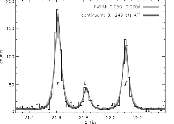
Figure 1: The spectral region including the O vii triplet. The light grey shade indicates the best fits when the background is fixed at 10 counts Å${}^{-1}$ and the line width is varied between values of 0.050 Å – 0.070 Å. The dark grey shade indicates the best fits when the line width is fixed at 0.053 Å and the background is varied between values of 0 – 249 counts Å${}^{-1}$.

In the X-ray spectra, the ratio of the fluxes in the forbidden line (f) (1s2s ${}^{3}$S – 1s${}^{2}$ ${}^{1}$S) and the intersystem line (i) (1s2p ${}^{3}$P${}_{1,2}$ – 1s${}^{2}$ ${}^{1}$S) in the He i-like ions is potentially sensitive to $n_{\rm e}$ (gj69). Of the He i-like ions observed with the LETGS, only O vii has lines that are sufficiently strong and unblended to use in a measurement of $n_{\rm e}$. Because of the importance of the measured flux ratio we have varied the continuum level and line widths used in extracting the fluxes, in order to obtain realistic error bars. The spectrum and these fits are shown in Fig. 1. The mean observed ratio is 2.88 ${}^{+0.57}_{-0.34}$. Provided the same widths are used for both lines, uncertainties in the widths have less effect than those in the choice of continuum. The range of the observed ratio is 2.535 – 3.455, compatible with the ratio of 3.06 measured by sf04, who allowed explicitly for contributions from what they regarded as weak unidentified lines.

Using CHIANTI (v4.2), at $T_{\rm e}=2\times 10^{6}$ K, the observed ratio of 2.88 leads to $\log P_{\rm e}=16.35$, with a range of 16.54 – 16.00. The lower limit is consistent with the pressure found from the transition region lines at $\log T_{\rm e}=5.3$. This pressure is essentially the same as the value of $\log P_{\rm e}=16.33$ found in an earlier analysis by ness02, which was adopted by sf04. (Using atomic data from APED gives essentially the same results.) CHIANTI (v4.2) predicts a ratio of 3.9 in the low-density limit, but does not include recombination to the n = 2 levels, either directly or via cascades. Early work by gj73 showed that including both radiative and di-electronic recombination tends to increase the predicted ratio in the low-density limit, but by only a relatively small amount; collisional excitation followed by cascades is more important. They predicted a low-density limit of 3.64. blum72 found larger effects from recombination, but according to gj73 they overestimated the contributions from di-electronic recombination.

The most recent version of CHIANTI (v5.2) gives the option of including radiative recombination as a process populating the excited states. The implementation of radiative recombination in CHIANTI (v5.2) is not correct, since it does not take into account recombination to the 1s2p ${}^{3}$P${}_{0}$ level (landi06) and hence omits an important process for populating the 1s2s ${}^{3}$S level. This leads to lower values of the f/i ratio at a given value of $n_{\rm e}$. In particular, the value of f/i at low densities ($R_{o}$) becomes $\simeq 3.35$.

pordu00 have given radiative and di-electronic recombination rate coefficients and effective collision strengths for populating the n = 2 levels, including the effects of cascades from n $>$ 2 in all cases. At $\log T_{\rm e}=6.3$ their calculations predict a value of $R_{o}=3.82$, a little smaller than that found from CHIANTI (v4.2). Compared with the work by gj73, pordu00 find larger contributions from collisional excitations, followed by cascades, to levels with n $>$ 2. Using the calculations by pordu00 (but neglecting the small contribution from recombination, since this causes only a small increase in $R_{o}$) leads to pressures that are similar to those from CHIANTI (v4.2) ($\log P_{\rm e}=16.38$, with a range from 16.56 to 15.93). Here the lower limit is compatible with the pressure found at around $\log T_{\rm e}=5.3$, without considering the error bars.

At present, the origin of the higher optimum pressure found from the O vii lines is not clear, but we think that it is in part due to remaining uncertainties in the atomic data, as well as those in the flux measurements. A fuller atomic model for the He i-like ions is clearly needed in CHIANTI. Ideally, the value of $R_{o}$ should be established from observations of the quiet solar corona, where the density is expected to be sufficiently low to give this limiting ratio. gj73 used an observed ratio of 3.6 in this manner, although blum72 quote higher ratios of 3.78 and 3.92. Unfortunately, the LETGS spectra of $\alpha$ Cen A (ness02), where a solar-like pressure might be expected, do not have sufficient flux in the O vii lines to measure $R_{o}$ to within useful limits.

The EUVE lines of Fe xiv are formed around $\log T_{\rm e}=6.25$, within the range over which the O vii lines are formed. laming96 found $\log P_{\rm e}=15.25$ from the lines at 211.33 Å and 219 Å, but the latter is weak and blended. Using the 211.33-Å and 264.78-Å lines, schmitt96 found $\log P_{\rm e}=15.55$, still lower than that indicated by the O vii and transition region lines.

A number of other line ratios are sensitive to $n_{\rm e}$, because the relative populations of the levels in the ground term are not given by the Boltzmann population (e.g. lines in the B i-like isoelectronic sequence and lines of iron). The densities derived depend on the overall form of the EMD and relative element abundances and are discussed in Section 4.5 and Section 4.6.1.

In the calculations that follow in Sections 4 and  LABEL:S5 we have explored the results using pressures of $\log P_{\rm e}=15.30$, 15.68 and 16.10. In Section LABEL:S6 we require the theoretical models to produce a value of $\log P_{\rm e}=15.97\,\pm\,0.20$ at $\log T_{\rm e}=5.3$.

4 Emission measure loci and line identifications

The identifications of the strong lines in the LETGS range are well known. In identifying other lines, and to check for blends, we used both APED (ATOMDB v1.3.1) and the CHIANTI database (v5.2) (landi06) to explore which transitions might be present at a given wavelength. Emission measure loci (EMLs) were then calculated for possible candidates, including any dependence on $P_{\rm e}$.

For a spherically symmetric atmosphere, the line flux observed at the Earth is given by

$$F_{21}=\frac{R_{*}^{2}}{d^{2}}\frac{hc}{\lambda}\frac{n_{E}}{n_{\rm H}}\int\frac{n_{2}}{n_{ion}}\frac{A_{21}}{n_{\rm e}}\frac{n_{ion}}{n_{\rm E}}G(r)f(r)n_{\rm e}n_{\rm H}{\rm d}r$$ (1)

where $G(r)$ is the fraction of photons not intercepted by the star, $f(r)=r^{2}/R_{*}^{2}$ and $d$ is the distance to the star. The excited and lower levels are $2$ and $1$, respectively (where $1$ is not necessarily the ground state); $n_{E}/n_{\rm H}$ is the abundance of the element relative to hydrogen, taken as constant over the region of line formation; $n_{ion}/n_{E}$ is the relative ion population; $n_{\rm H}$ is the hydrogen number density; $A_{21}$ is the spontaneous transition probability and the integration is over the radial distance, d$r$.

Equation (1) can be rewritten as

$$F_{21}\simeq g(n_{\rm e},T_{\rm e})\int n_{\rm e}n_{\rm H}G(r)f(r){\rm d}r$$ (2)

where $g(n{\rm e},T_{\rm e})$ includes all other terms in equation (1). Provided any dependence on $P_{\rm e}$ is taken into account, the emission measure locus (EML) gives the value of the apparent emission measure ($EM=\int n_{\rm e}n_{\rm H}~{}G(r)~{}f(r)$ d$r$) that would be required to account for all the observed flux, at each value of $T_{\rm e}$ in turn. The loci therefore provide useful constraints on the mean EMD, since if this exceeds the minimum of a locus by more than a small factor, too much flux will be predicted when the mean EMD is used to predict the line fluxes.

It is important to note that loci from lines of different isoelectronic sequences can have different variations of $g(T_{\rm e})$ with $T_{\rm e}$, owing to the systematic differences in $n_{ion}/n_{E}$ as a function of $T_{\rm e}$. Otherwise, if a line with a broad $g(T_{\rm e})$ function were compared with one with a narrow $g(T_{\rm e})$ function, an incorrect relative element abundance would be deduced. These differences are taken into account in finding the mean EMD (see Section LABEL:S5).

Values of $n_{2}A_{21}/n_{\rm e}$ have been calculated using CHIANTI (v5.2). The relative ion populations for iron have been taken from aray92. For O vi, the calculations given in simjordan05 have been adopted, since these include the density dependence of di-electronic recombination. All other values are taken from arot85. The element abundances initially adopted and the corrections to these required by the observations are discussed in Section LABEL:S5.

The lines of elements other than iron are now discussed according to their isoelectronic sequence. Comparisons have been made between observed and predicted line flux ratios (or relative EMLs) using a single temperature for the line formation and also using the total fluxes predicted using the final EMD. Unless otherwise stated, both approaches give the same results. Although only the lines that we regard as the most reliable are used to determine the mean EMD, we calculate the predicted fluxes in all the lines discussed below and later compare these with the observed fluxes.

4.1 Hydrogen-like lines

The (unresolved) Lyman $\alpha$ lines of C vi, N vii, O viii, Ne x and Mg xii are all observed, although the Mg xii lines are weak. The Ne x lines at 12.13 + 12.14 Å are blended with a line of Fe xvii at 12.12 Å. Another line of Fe xvii is observed at 12.27 Å. The ratio of these two Fe xvii lines does not depend significantly on $T_{\rm e}$ so we have used the line at 12.27 Å to predict the flux in the line at 12.12 Å. This results in 73 per cent of the observed total flux in the line at 12.13 Å being due to Ne x.

The Lyman $\beta$ lines are observed in O viii (at 16.01 Å) and Ne x (at 10.23 Å), but the former is blended with a line of Fe xviii at 16.00 Å. Another line of Fe xviii at 16.07 Å has been used to find the contribution of the 16.00-Å line to the total flux. The ratio of the Fe xviii lines is slightly sensitive to $T_{\rm e}$, and their temperature of optimum formation could lie between $\log T_{\rm e}=6.5$ and 6.8. The total predicted fluxes show that 81 per cent of the observed line at 16.01 Å is due to O viii. The ratio of the observed flux in O viii Lyman $\beta$ to that in the Lyman $\alpha$ line is then a factor of 1.2 larger than that predicted using the mean EMD. In Ne x, the observed Lyman $\beta$ to Lyman $\alpha$ ratio is a factor of 1.4 larger than predicted.

4.2 Helium-like lines

The resonance (r), intersystem (i) and forbidden line (f) of C v lie in a region of low and rapidly varying effective area and a real signal is observed only in the r line at 40.27 Å. However, this is slightly blended with the third order of the Ne ix r-line and it is hard to determine a reliable flux (ness01). The uncertainty in the flux given in Table 3 includes the results of varying the background and line width. The r-line of N vi is present, although rather weak; the i and f-lines are not sufficiently above the local noise level to be useful. The lines of O vii are relatively strong and their use in constraining $P_{\rm e}$ has been discussed in Section 3. Note that the contribution from radiative recombination has been included when predicting the fluxes in the singlet lines of all the He i-like ions.

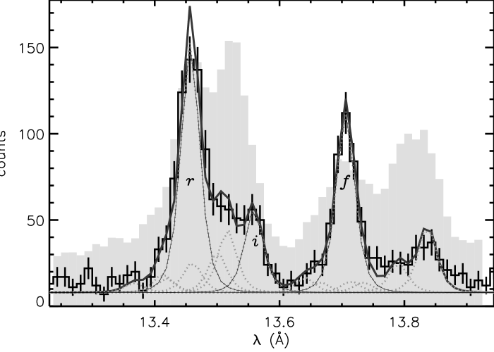
Figure 2: The spectral region around the Ne ix triplet in $\epsilon$ Eri and Capella (light grey shade), rescaled to match the peak flux in the r line. The contributions from the lines of Fe xvii, xviii and xix in $\epsilon$ Eri are shown by dotted lines. Those for the r, i and f lines are shown by full lines. The blending in $\epsilon$ Eri is clearly far less severe than in Capella. The method of fitting is described in the text. The fluxes derived for the Ne ix lines, and their uncertainties, are given in Table 3.

The lines of Ne ix are also relatively strong, but are blended to various degrees with lines of Fe xvii, xviii and xix. A comparison between the LETGS spectra of $\epsilon$ Eri and Capella, shown in Fig. 2, indicates that the blends with lines of iron are less important than in Capella. In $\epsilon$ Eri, the Fe xvii line at 13.83 Å is significantly weaker than the Ne ix f line and the Fe xix + xxi blend at 13.51 Å is significantly weaker than the r line. The de-blending problem is therefore less severe than in Capella. The procedure used is as follows: the amplitudes and wavelengths of the lines observed in Capella using the High Energy Transmission Grating Spectrograph (HETGS) (see ness03a) are used to predict the counts in the LETGS spectra, taking into account the resolution and effective area of the LETGS; the lines of Fe xvii and Fe xviii are grouped together, as are the lines of Fe xix, while the lines of Ne ix are treated individually; the amplitudes of the 2 groups and 3 individual lines are scaled iteratively to obtain the best fit to the LETGS spectrum of $\epsilon$ Eri and hence the fluxes in the Ne ix lines are determined. The fits made are shown in Fig. 2. The analyses of all lines of neon and other lines of iron shows that the relative weakness of the blended iron lines in $\epsilon$ Eri arises from both the lower EMD above $\log T_{\rm e}=6.6$ and a lower Fe/Ne relative abundance. Given the de-blending process, in particular for the i-line, it is difficult to make a reliable interpretation of the relative fluxes in the Ne ix r, i and f lines.

The r and f lines are present in Mg xi and Si xiii, but the i lines cannot be distinguished. In extracting fluxes we have summed over the r, i and f lines. The predicted fluxes are lower limits, since the contribution to the populations of excited states from dielectronic recombination is not yet included in CHIANTI (v5.2), and contributions from satellite lines are not yet included for Mg xi.

The 1s3p ${}^{1}$P – 1s${}^{2}$ ${}^{1}$S transition in O vii is present as a weak line at 18.63 Å, but is blended with a weaker line. The same transition in Ne ix might also be present at 11.54 Å. These weak lines are not used in deriving the mean EMD.

4.3 Lithium-like lines

In the region below 170 Å the transitions observed in the Li i-like ions are those between the n = 3 and n = 2 levels (3p – 2s, 3d – 2p, 3s – 2p). The 3p – 2s (unresolved) lines in O vi at 150.1 Å are present in the minus direction spectrum, but are barely above the instrumental noise level in the plus direction spectrum. The measured flux is very sensitive to the background adopted and provides only an upper limit to the EML. Although the 3p – 2s lines are not included in the derivation of the mean EMD, this reproduces the observed flux to within a factor of 1.1. The 2p – 2s transitions are both observed (around 1032 Å and 1038 Å) in spectra obtained with FUSE in 2000 December. They are useful in constraining the EMD between $\log T_{\rm e}=5.5$ and 6.1 (see Section LABEL:S5).

In Ne viii the 3p – 2s and 3d – 2p transitions are observed at around 88.1 Å and 98.2 Å, respectively. Although the 3s – 2p transitions are just present around 103.1 Å, they are too weak to yield a reliable flux. The 4d – 2p transitions occur around 73.5 Å  but on the basis of the calculated EMLs, the line observed is identified as one of Fe xv. heroux72 suggested that in the solar spectrum, the lines around 88.1 Å are blended with lines of Fe xi and identify a line at 86.88 Å with the strongest member of the multiplet (at solar densities). At the higher value of $n_{\rm e}$ in $\epsilon$ Eri, the line at 86.88 Å should still be the strongest member of the multiplet, but is not observed. We have rejected the possibility of a second order line of Si xii at 88.04 Å because a stronger second order Si xii line at 88.34 Å is not present. Thus significant blending with these Ne viii lines seems unlikely. Note that the relevant lines of Fe xi are not yet included in either CHIANTI or APED. heroux72 also suggested that both of the lines at 98.11 Å and 98.26 Å are blended with other lines in the solar spectrum. In $\epsilon$ Eri, to within the measurement uncertainties, the two lines have the expected wavelength separation and almost the theoretical flux ratio, so there is no obvious evidence of substantial blending.

The lines in Mg x are all weak. The 3p – 2s multiplet at 57.90 Å is not resolved; only the summed flux is used. The 3d – 2p transitions at 63.30 Å + 63.31 Å and 63.16 Å are observed only in the minus direction spectrum, owing to a chip gap in the plus direction. We use only the blend of transitions at around 63.3 Å in deriving the EMD, since the weaker line at 63.16 Å is barely above the noise level. The 3s – 2p lines at 65.67 Å and 65.85 Å have an incorrect flux ratio in the minus side spectrum and summed spectra, suggesting that the intrinsically weaker line at 65.67 Å is blended. Also, the line at 65.85 Å might be blended with another line at around 65.93 Å  making it difficult to extract a reliable flux; these two Mg x lines are excluded from the derivation of the mean EMD.

In Si xii the 3p – 2s lines lie around 40.93 Å  in the region of the instrumental absorption edge, and are not observable. The 3d – 2p transitions at 44.02 Å and 44.17 Å are observed as moderately strong lines. The observed ratio of the stronger to weaker components is about 1.5, instead of the predicted value of 1.99. We use only the stronger line, on the grounds that the weaker line might be blended. The 3s – 2p lines at 45.52 Å and 45.69 Å are also observed, but are not used in deriving the mean EMD, as they are weak and blended with other weak lines or instrumental noise.

There are weak lines that are possibly due to S xiv. A line at 32.56 Å corresponds to the stronger component of the 3d – 2p transitions. Another at 30.46 Å corresponds to the 3p – 2s transitions, but the 2p${}^{5}$3d ${}^{1}$P – 2p${}^{6}$ ${}^{1}$S transition in Ca xi occurs at 30.47 Å and could contribute to the measured flux. These lines were not used in deriving the mean EMD.

In Ne viii the ratio of the observed flux from the 3p – 2s transitions to that in the 3d – 2p transitions is about a factor of 1.5 larger than predicted. This suggests that the atomic models or atomic data for the lithium-like ions would bear closer examination.

4.4 Beryllium-like lines

No lines of Mg ix are observed. Because it is useful to constrain the EMD at around $10^{6}$ K, we have used the background level at 72.31 Å and 77.74 Å (the wavelengths of the 2s3d – 2s2p and 2s3s – 2s2p transitions, respectively), to find the upper limit to their EMLs.

Three singlet lines of Si xi are observed; the 2s3p – 2s${}^{2}$ line at 43.76 Å, the 2s3d – 2s2p line at 49.22 Å and the 2s3s – 2s2p line at 52.30 Å (but the latter only in the plus side spectrum). Only the 52.30-Å line appears to be unblended.

The strongest transition (2s3d – 2s2p) in S xiii is observed at 35.67 Å; other transitions are present, but are barely above the noise level.

4.5 Boron-like lines

The 3d – 2p lines of Si x lie at 50.69 Å (${}^{2}$P${}_{3/2}$ – ${}^{2}$D${}_{5/2,3/2}$) and 50.52 Å (${}^{2}$P${}_{1/2}$ – ${}^{2}$D${}_{3/2}$). As in Fe xiv (jordan65), the ratio of these lines depends on $n_{\rm e}$, since the relative populations of the ground ${}^{2}$P levels have a Boltzmann distribution only at large values of $n_{\rm e}$. The line at 50.52 Å is blended with a line of Fe xvi at 50.55 Å and careful deblending is required. Using the procedure described in Section LABEL:S4.6.3, the ratio of the deblended fluxes in the 50.69 and 50.52-Å lines is $1.52\,\pm\,0.26$. Using CHIANTI (v5.2) and the mean EMD, the predicted integrated fluxes give ratios of 1.51 at $\log P_{\rm e}=15.68$, 1.18 at $\log P_{\rm e}=15.30$ and 1.78 at $\log P_{\rm e}=16.10$. Thus a value of $\log P_{\rm e}$ close to 15.68 gives the best fit, but the uncertainty in the flux ratio just includes $\log P_{\rm e}=16.10$. The flux in the unblended Si x line at 50.69 Å is also weakly dependent on $n_{\rm e}$ (compared with the $n_{\rm e}^{2}$ dependence of most lines). At $\log P_{\rm e}=15.68$, the flux predicted by CHIANTI (v5.2) is a factor of 1.3 larger than that observed and a pressure of $\log P_{\rm e}\leq 15.30$ would be required to fit the observed flux. Predicted flux ratios are in general more accurate than absolute fluxes, since they do not depend on abundances or ion fractions, so there may be small problems with the atomic data.

The corresponding lines of S xii are not observed.

4.6 Lines from iron ions

We now discuss the lines of iron according to their stage of ionization.

4.6.1 Fe ix to Fe xiv

For these ions we rely on the $\Delta n=0$ transitions observed with the EUVE, although the Fe ix line is also observed with the LETGS. We also discuss the Fe xii forbidden lines that are observed with the STIS. At present, neither CHIANTI (v5.2) nor APED include all transitions of the type $\Delta n=1$ in these ions. We have updated earlier calculations of the EMLs by using CHIANTI (v5.2) (including those by simjordan03a, who used CHIANTI v4).

The lines of Fe ix to xiv used are all sensitive to $n_{\rm e}$, either through the departure from Boltzmann populations in the levels of the ground term, or from the population of higher metastable states. Apart from the blended lines of Fe xiii at 203.83 Å  the derived EMLs all increase with increasing $n_{\rm e}$. The stronger 203.83-Å line ends on an excited level of the ground term and thus has the opposite behaviour. To give a smoothly increasing EMD from all the lines of Fe x to xv would require a value of $\log P_{\rm e}\leq 15.30$; at higher pressures the Fe xiii locus lies below the mean value. Since there is no other evidence of such a low pressure, there might be small problems with the atomic data for Fe xiii in CHIANTI (v5.2) or in the EUVE line fluxes. With the inclusion of more levels in the atomic models of these ions, it might be possible to derive a value of $P_{\rm e}$.

The resonance line of Fe ix at 171.07 Å leads to a relatively low EML, irrespective of pressures in the range from $\log P_{\rm e}=$ 15.3 to 16.1. Even at $\log P_{\rm e}=16.10$, the mean EMD leads to a flux that is larger than the value observed with the EUVE by a factor of 1.8. The 171-Å line falls near the long wavelength limit of the LETGS and the short wavelength limit of the EUVE medium wavelength spectra; for both instruments there are significant uncertainties in the flux calibration at 171 Å and these could be one origin of the above discrepancy. As discussed by laming96, the ion balance calculations by arot85 lead to a larger EML than that found from the calculations by aray92. Near the peak emissivity, the difference between these calculations is a factor of 1.6, which would remove much of the discrepancy. However, the calculations by aray92 are expected to be more accurate. The final model can be used to estimate the line centre opacity. This is close to 1; although scattering of photons out of the line of sight could occur, detailed radiative transfer calculations are needed to find the effect on the spatially integrated line fluxes.

The atomic data for Fe xii have been revised since the work by jordan01a; jordan01b, who used CHIANTI (v3.01), and by simjordan03a, who used CHIANTI (v4.2). We have therefore re-examined the difference between the fluxes predicted by CHIANTI (v5.2) for the forbidden lines at 1242 and 1349 Å and the EUVE lines in the blend around 196 Å. For the lines at 1242 Å and at around 195 Å, jordan01a found a difference of a factor of 3 between their EMLs. This is now reduced to a factor of 1.8 (at $\log P_{\rm e}=15.68$) or 2.2 and 1.5 (at $\log P_{\rm e}=15.30$ and 16.10, respectively). The small dependence on $P_{\rm e}$ arises from a small increase in the forbidden line fluxes, and a small decrease in the EUV line fluxes, with increasing $P_{\rm e}$. Using the absolute line fluxes and the mean EMD, the agreement between the observed and predicted fluxes for the EUV lines is very good (to within a factor of 1.1 over the above range of $P_{\rm e}$) but the flux in the line at 1242 Å is predicted to be smaller than that observed, by the factors given above. Although differences in the fluxes arising from the different dates of the observations cannot be ruled out, neither can small corrections to the level populations for the forbidden lines (see below).

The ratio of the fluxes in the Fe xii forbidden lines at 1242 Å and 1349 Å is insensitive to $\log P_{\rm e}$ over the range from about 15.0 to 16.0, but is useful in placing an upper limit on $P_{\rm e}$. In $\epsilon$ Eri the observed ratio is 1.88 ($\pm\,0.2$) (and other main-sequence stars show a similar ratio) (jordan01a). Using a single temperature of $\log T_{\rm e}=6.15$, CHIANTI (v3.01) leads to $\log P_{\rm e}=15.72$, with an upper limit of 16.17. CHIANTI (v4.2) leads to $\log P_{\rm e}=15.53$, with an upper limit of 16.07. But CHIANTI (v5.2) leads to a pressure of $\log P_{\rm e}=14.21$, which is much lower than the transition region pressure found in Section 3. The upper limit is 15.80, which is consistent with the transition region pressure (15.97 $\pm 0.20$), but not with the pressure of $\log P_{\rm e}=16.14$ found in the final model at $\log T_{\rm e}=6.15$. At present we suggest that the atomic data used in CHIANTI (v3.01) or (v4.2) give a better fit to the forbidden line flux ratio than do those in CHIANTI (v5.2) (see storey05).

The value of the Fe xii forbidden line flux ratio provides a very sensitive test of the atomic data for these lines. E.g. jordan01b pointed out that the ratio of 2.7 predicted by binello01 could not be correct. It is also of interest to compare the population of the 3p${}^{3}$ ${}^{2}$P${}_{1/2}$ level from CHIANTI (v5.2) with that predicted empirically by gj75 on the basis of solar observations. At $T_{\rm e}=1.65\times 10^{6}$ K and $n_{\rm e}=3\times 10^{8}$ cm${}^{-3}$, CHIANTI (v5.2) gives a level population (relative to that of the ion) of $2.9\times 10^{-4}$, whereas the solar observations led to values between 3.3 and 5.1 $\times 10^{-4}$. Thus there is other observational support for a larger ${}^{2}$P${}_{1/2}$ population.

Given that the final EMD peaks around the temperature where Fe xv and xvi are formed, one might expect lines of Fe xiv to be present in the X-ray region. There are four weak lines around 76 Å that are also present in the LETGS spectra of Procyon (raassen02), $\alpha$ Cen A and B (raassen03) and Capella (sf04). In $\epsilon$ Eri the lines are at 75.91 Å, 76.04 Å, 76.13 Å and 76.53 Å. We propose that the lines at 76.04 Å and 76.13 Å are due to the 3d ${}^{2}$D – 4f ${}^{2}$F transitions in Fe xiv, but owing to the absence of these lines in CHIANTI or APED we cannot check this through derived EMLs. raassen03 have also proposed this identification for lines in $\alpha$ Cen A and B. In Procyon, a line at 75.98 Å may well be due to Fe x (raassen02), but in $\epsilon$ Eri the EMD is relatively smaller where such lines are formed. Using our final EMD, none of the four possible lines of Fe xiv between 75.69 Å and 76.82 Å are predicted to be observable. A line of Fe xvi occurs at 76.50 Å but the next strongest member of the multiplet at 76.80 Å is absent (see also Section 4.6.3).

4.6.2 Fe xv

The resonance line at 284.2 Å is observed as a strong line with the EUVE. Using our final EMD, the flux predicted in this line is a factor of 1.16 larger than that observed. Possible sources of uncertainty include the amount of absorption by the ISM and line opacity effects.

The X-ray spectrum of Fe xv in a solar flare and Capella has been discussed by keenan06 and we make comparisons with predicted flux ratios at $\log T_{\rm e}=6.3$ (near where the EMLs for the Fe xv lines have their minimum value) and $\log T_{\rm e}=6.5$ (to allow for the increase in the mean EMD). We also make comparisons with the flux ratios predicted using CHIANTI (v5.2) and the mean EMD. We observe only singlet transitions whose flux ratios do not depend on $n_{\rm e}$.

The 3s4d ${}^{1}$D – 3s3p ${}^{1}$P (59.40 Å) transition is adopted as the standard line. The blend at 59.27 Å observed in Capella by keenan06 is not obvious in $\epsilon$ Eri, consistent with their suggestion that it is due to Fe xvii. The 59.40-Å line flux is a factor of 1.38 larger than that predicted using CHIANTI (v5.2) and the mean EMD.

The 3s4p ${}^{1}$P – 3s${}^{2}$ ${}^{1}$S transition at 52.91 Å is not obviously blended in $\epsilon$ Eri, unlike the situation in Capella. The observed flux ratio agrees well with that predicted using CHIANTI (v5.2), and although the flux ratio from keenan06 is smaller, it also agrees with that observed to within the uncertainties.

The strongest X-ray line is both predicted and observed to be the 3s4s ${}^{1}$S – 3s3p ${}^{1}$P transition at 69.68 Å. In $\epsilon$ Eri this line is blended with one at around 69.6 Å that does not appear to be present in Capella ((keenan06)). We note that kelly87 lists predicted lines of Fe xiv in this region. The flux ratio observed for the line at 69.68 Å is a factor of about 1.5 lower than that predicted by both CHIANTI (v5.2) and keenan06, which agree well with each other. This ratio is also lower than expected in Capella, but agrees with the theoretical value to within the uncertainties.

The 3s4f ${}^{1}$F – 3s3d ${}^{1}$D transition occurs at 73.47 Å, but is potentially blended with a line of Ne viii at 73.48 Å. Interpreting the observed line flux as being due entirely to Ne viii, using CHIANTI and the mean EMD gives an observed to predicted flux ratio that is a factor of 4.0 too large. Assuming that the predicted Ne viii flux is correct, its contribution can be removed to give an Fe xv flux of $2.04\times 10^{-14}$ erg cm${}^{-2}$ s${}^{-1}$ and a flux ratio of 0.68. The temperature sensitivity of the Fe xv 73.47-Å line is not given by keenan06 so that of the triplet lines from the same configuration has been used to find the expected flux ratio at $\log T_{\rm e}=6.50$. This corrected flux ratio agrees well with the flux ratio predicted by keenan06, but the flux ratio predicted using CHIANTI is larger. However, the stronger member of the Ne viii multiplet that should occur at 73.56 Å is not present with the flux expected from CHIANTI. For this reason we have also found the observed flux ratio assuming no contribution from Ne viii, and this agrees with that predicted using CHIANTI, to within the uncertainty.

The predicted and observed flux ratios are summarized in Table 5. We have checked that the uncertainties in the observed ratios also cover the range of values derived using a range of background levels. Of the X-ray lines, only the observed flux ratio for the line at 69.68 Å is discordant with the calculations. On average, the flux ratios predicted by keenan06 are smaller than those predicted using CHIANTI (v5.2).

At present, the atomic model does not include levels with $n$ larger than 5; this could be one cause of the remaining differences between the observed and calculated flux ratios for transitions from the $n=4$ levels. Also, from section 2.3 of landi06, the effects of recombination and ionization on the populations of excited states have not yet been included for Fe xv.

Table 5: Fe xv line flux ratios, relative to the flux in the 59.40-Å line${}^{a}$.

Line	Keenan et al.	CHIANTI (v5.2)${}^{b}$	Observed
(Å)	(2006)
	$\log T_{\rm e}$
52.91	6.3   $0.65\,\pm\,0.13$	0.81	$0.75\,\pm\,0.17$
	6.5   $0.64\,\pm\,0.13$
69.68	6.3   $3.1\,\pm\,0.6$	2.75	$1.85\,\pm\,0.31$
	6.5   $2.7\,\pm\,0.5$
73.47	6.3   $0.97\,\pm\,0.16$	1.01	$0.68\,\pm\,0.20$${}^{c}$
	6.5   $0.75\,\pm\,0.12$		$0.91\,\pm\,0.22$${}^{d}$
284.2		56.0	$34.8\,\pm\,5.6$

${}^{a}$ This is $2.99\,\pm\,0.44\times 10^{-14}$ erg cm${}^{-2}$ s${}^{-1}$, when corrected for absorption in the ISM.
${}^{b}$ Predicted using the mean EMD (see Table 10), using $\log P_{\rm e}=16.10$.
${}^{c}$ With the predicted contribution from Ne viii removed.
${}^{d}$ Assuming no contribution from Ne viii.