ECHO EMISSION FROM DUST SCATTERING AND X-RAY AFTERGLOWS OF GAMMA-RAY BURSTS

Abstract

We investigate the effect of X-ray echo emission in gamma-ray bursts (GRBs). We find that the echo emission can provide an alternative way of understanding X-ray shallow decays and jet breaks. In particular, a shallow decay followed by a “normal” decay and a further rapid decay of X-ray afterglows can be together explained as being due to the echo from prompt X-ray emission scattered by dust grains in a massive wind bubble around a GRB progenitor. We also introduce an extra temporal break in the X-ray echo emission. By fitting the afterglow light curves, we can measure the locations of the massive wind bubbles, which will bring us closer to finding the mass loss rate, wind velocity, and the age of the progenitors prior to the GRB explosions.

1 INTRODUCTION

Gamma-ray bursts (GRBs) are the most luminous and intriguing explosions in the universe. A number of physical interpretations for GRBs have been proposed since they were discovered about four decades ago. The most successful model for GRBs and their afterglows is the fireball shock model (Mészáros, 2006, and references therein). Although the interpretation for the prompt gamma-ray emission is still controversial even in this standard scenario, the long-wavelength afterglows have been widely accepted to be the emission from relativistic shocks sweeping up an external medium (Mészáros, 2006; Zhang, 2007, and references therein).

In spite of the success of the standard external shock model for interpreting most features of afterglows, there are still a few issues recently raised by the Swift X-ray Telescope (XRT) (Gehrels et al., 2004). The first issue is the ubiquitously detected shallow decay of early X-ray afterglows (Nousek et al., 2006; Zhang et al., 2006). In general, to account for the shallow decay, a “refreshed shock” scenario is assumed, either by a continuous activity of the GRB progenitor (Dai & Lu, 1998; Zhang, & Mészáros, 2001; Dai, 2004), or by a power-law distribution of the Lorentz factors in the ejecta (Rees & Mészáros, 1998; Sari & Mészáros, 2000). However, although the “refreshed shock” model is generally able to explain the flatter temporal X-ray slopes from current analysis, it may not be able to explain self-consistently both the X-ray and the optical afterglows of some well-monitored GRBs, such as GRB 050319 and GRB 050401 (Fan & Piran, 2006).

The second issue is the lack of jet breaks that are supposed to be detected simultaneously in X-ray and optical light curves (Panaitescu et al., 2006; Sato et al., 2007; Burrows & Racusin, 2007). This raises a serious concern about our understanding of the afterglow emission. Currently, possible solutions to this problem are additional mechanisms taking place in the early X-ray emission (Fan & Piran, 2006), X-ray emission arising from different outflows with the optical emission (Panaitescu et al., 2006), or alternatively, the temporal break in X-rays is masked by some additional source of X-ray emission (Sato et al., 2007), so that a jet break at the expected time could still be seen in the optical band. The last interpretation may bring renaissance to the physical meaning of a jet break (Rhoads, 1999) and $E_{\rm jet}$ (Frail et al., 2001), and therefore revive the relation between $E_{\rm jet}$ and $E_{\rm peak}$ (Ghirlanda et al., 2004).

Recently Shao and Dai (2007) realized that the impulsive prompt X-ray emission scattering off the surrounding medium could give rise to a long-term X-ray flux, which is comparable to that of most observed afterglows. The scattered X-ray emission (which is called echo emission herein) could be an additional contributor to the early X-ray afterglow, which was originally put forward by Klose (1998) and then further discussed by Mészáros & Gruzinov (2000) and Sazonov & Sunyaev (2003). Shao and Dai (2007) also worked out detailed light curves of the echo emission that could nicely reproduce most of the temporal features of observed X-ray afterglows, i.e., a shallow decay followed by a “normal” decay and a further rapid decay (Zhang et al., 2006; Nousek et al., 2006). This scenario provides a self-consistent solution to both the shallow decay and the jet break problem. By fitting the X-ray light curves of GRB 060813 and GRB 060814, Shao and Dai (2007) concluded that the scattering medium, i.e., a dusty shell should be at a distance of about tens of parsecs from the GRB source.

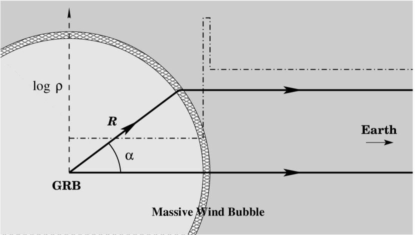
Figure 1: Geometry and density profile of a massive wind bubble around a WR star. The major scattering takes place at the massive and dense shell (marked with brick-wall pattern), which is a main dusty shell around the WR star (or more probably a WC star). Inside the shell, the interior structure of the bubble (filled with light gray) is ignored, which is mainly determined by the LBV and WR winds and not important for scattering, since the density is much lower there and essentially no dust survives close to the WR star. Outside the shell, the interstellar medium (ISM) dominates (filled with heavy gray). Meanwhile, the gas density $\rho$ is also plotted with logarithmic scale in dot-dashed line (not in scale, see García-Segura et al., 1996a; Dwarkadas, 2007).

Coincidentally, this conjectured dusty shell by Shao and Dai (2007) is consistent with the massive wind bubble around a Wolf-Rayet (WR) star, which has been proposed as the progenitor of a GRB. The study of stellar structure and evolution has provided a mass-loss history of a massive star, starting with the Main Sequence (MS) stage as an O star, which will evolve into a WR star and then produce a final supernova and/or a GRB. By the computation of stellar wind and atmosphere models for a O-type star of 60 ${\rm M_{\sun}}$ mass, Langer et al. (1994) concluded that the stellar mass lost to the wind bubble is about 32 ${\rm M_{\sun}}$ in the MS stage, 8 ${\rm M_{\sun}}$ in the Luminous Blue Variable (LBV) stage, and 16 ${\rm M_{\sun}}$ in the WR stage. Such a massive wind bubble will produce a significant shell mainly swept up by the MS wind at the time of the supernova or GRB (see Fig.1), with a distance from the progenitor of about $R\sim$ tens of parsecs (García-Segura et al., 1996a; Mirabal et al., 2003; Dwarkadas, 2007). If the clumps formed during the LBV and WR stages survive long enough, they will be hitting the MS shell roughly at the time of the supernova or GRB (García-Segura et al., 1996a).

In this paper, we apply the echo emission model to a sample of 36 GRBs with well-monitored X-ray light curves by the XRT onboard Swift. We find that most of the light curves without significant flares can be reproduced by our model. In this sample, 14 bursts have available redshifts by observations. By fitting their X-ray light curves, we find the distance $R$ of the wind bubbles from GRB progenitors. A measurement of $R$ might bring us closer to finding the mass loss rate, density and wind velocity of the progenitor prior to the explosion.

Our paper is structured as follows: In $\S$2, we first discuss the existence of massive stellar wind bubbles around GRBs when they explodes and the subsequent X-ray echo emission. We formulate the theoretical light curves of X-ray echo emission in $\S$3, and we introduce the temporal break in echo emission and fit the observational light curves of 36 GRBs in $\S$4. Discussion and conclusions follow in $\S$5.

2 THE ECHO ON THE BUBBLE

It has been shown by Shao and Dai (2007) with a detailed calculation following Miralda-Escudé (1999) that, the fiducial flux of the echo emission could be comparable to an already observed X-ray afterglow at some certain time, given that the prompt X-rays from a GRB are significantly scattered by the circumstellar dust. Here, we provide a more concise approach by order-of-magnitude estimation.

Evidence accumulated in the last few years has verified the long-hypothesized origin of soft GRBs in the deaths of WR stars (Woosley & Bloom, 2006, and references therein). It is generally believed that the progenitor WR star will blow out a hot bubble in the interstellar medium (ISM) by massive stellar wind (García-Segura et al., 1996a; Dwarkadas, 2007). The typical radius of the dense shell of swept-up surrounding ISM is of order tens of parsecs, as given by a self-similar solution (Castor et al., 1975; Ramirez-Ruiz et al., 2001; Mirabal et al., 2003)

$$R = \left({25\dot{M}v^{2}}\over{14\pi nm_{\rm p}}\right)^{1/5}t^{3/5}$$ (1)

$$= 100\left({\dot{M}_{-6.2}v_{3.5}^{2}\over n_{0}}\right)^{1/5}t_{6.6}^{3/5}\,{\rm pc},$$

where the mass-loss rate during the MS stage $\dot{M}=10^{-6.2}\,{\rm M_{\odot}/yr}$, the typical wind velocity $v=10^{3.5}$ km/s, and the lifetime of the MS stage $t=10^{6.6}$ yr are adopted for a 35 ${\rm M_{\odot}}$ star (García-Segura et al., 1996b; Dwarkadas, 2007), and the number density of interstellar medium $n=1\,{\rm cm}^{-3}$ is assumed.

Correspondingly, the geometry and density profile of a massive wind bubble around a WR star are shown in Fig.1. WR stars – characterized by high mass-loss rate – are believed to form massive dust in their winds (e.g., Williams et al., 1987; Crowther, 2003, 2007). Interestingly, all dust shells that were observed were essentially associated with carbon-rich WR stars of the latest subtypes of the WC sequence only (which are called WC stars herein, e.g., Allen et al., 1972; Gehrz & Hackwell, 1974). WC stars are the final evolutionary phase of the most massive ($\geq 40{\rm M_{\sun}}$) stars, which, in some sense seem to be favored here as the progenitors of some GRBs, since there is where echo emission would be most efficient.

Assuming that an X-ray burst (i.e., the X-ray counterpart of a prompt GRB produced at the final stage of a WC star) with a fluence $S_{\rm X}$ is scattered by the dusty shell at a distance $R$ with a scattering optical depth $\tau_{\rm sca}$, the echo emission is spread within a characteristic time scale $t_{\rm d}$, due to the scattering delay of X-rays with different scattering angles $\alpha$ (see Fig.1 for the geometry of scattering). Since the characteristic scattering angle $\alpha$ is physically small (Alcock & Hatchett, 1978), the time scale $t_{\rm d}$ is consequently much smaller than $R/c$, where $c$ is the speed of light. Therefore, we have a fiducial flux of the X-ray echo emission over a time $T_{\rm d}$

$$F^{\rm echo} = {S_{\rm X}\times\tau_{\rm sca}\over t_{\rm d}}$$ (2)

$$= 2.5\times 10^{-11}\,\left({S_{\rm X}\over 2.5\times 10^{-7}\,{\rm ergs\,cm^{-2}}}\right)\left({\tau_{\rm sca}\over 0.1}\right)\left({t_{\rm d}\over 10^{3}\,{\rm s}}\right)^{-1}\,{\rm ergs\,cm^{-2}\,s^{-1}},$$

where $S_{\rm X}$ is the total fluence of the burst observed in X-ray band (say, 0.3-10 keV), the echo flux and the source flux are assumed to suffer the same interstellar absorption on their way to the observer, and the cosmological $k$-correction is ignored. $S_{[0.3-10]}=2.5\times 10^{-7}\,{\rm ergs\,cm^{-2}}$ is approximated here, assuming $S_{[0.3-10]}/S_{[15-150]}=1/4$ and $S_{[15-150]}=10^{-6}\,{\rm ergs\,cm^{-2}}$, given that $S_{[50-100]}/S_{[25-50]}\sim 1$ (Sakamoto et al., 2007) and most GRBs have a flat spectrum in soft X-ray band (Preece et al., 2000; Sakamoto et al., 2007). Note that, a realistic $S_{[0.3-10]}$ should be essentially larger than the value we adopt here, because the X-rays between [0.3-10] keV before and after the BAT trigger interval ($T_{100;}$ Sakamoto et al., 2007), especially those from the soft tail emission in most GRBs, are not included in this approximation. Since the scattering angle $\alpha$ is very small, we have

$$t_{\rm d} = {(1+z)R\alpha^{2}\over 2c}$$ (3)

$$= 10^{3}\,\left(1+z\over 2\right)\left(R\over 100\,{\rm pc}\right)\left({\alpha\over 1\arcmin}\right)^{2}\,{\rm s},$$

where $z$ is the redshift of the GRB, and $\alpha$ is the typical scattering angle of X-ray echo emission (Alcock & Hatchett, 1978; Klose, 1998).

Hence, we have three interesting coincidences:

1. The dusty shell at a distance $R$ of about tens of parsecs assumed by Shao and Dai (2007) is consistent with the massive wind bubble around a WR star at its final stage (García-Segura et al., 1996a; Mirabal et al., 2003; Dwarkadas, 2007);

2. The timescale of the X-ray echo emission on such a wind bubble is about $t_{\rm d}\sim 10^{3}$ s, which is the typical timescale when the shallow decay phase dominates in X-ray afterglow (Zhang et al., 2006; Nousek et al., 2006);

3. The X-ray echo flux $F^{\rm echo}$ from such a wind bubble is consistent with most of both pre-Swift and Swift X-ray afterglows around $10^{3}$ s (e.g., Costa, 1999; Nousek et al., 2006).

These three coincidences motivate the study of echo emission as an additional contributor to the X-ray emission. In what follows, we work out the light curve of the echo emission, and show the fourth and the most spectacular coincidence that the theoretical light curves of X-ray afterglows are consistent with the observed ones.

3 THEORETICAL LIGHT CURVE

Shao and Dai (2007) have derived the temporal profile of the echo emission. They showed that the feature in the X-ray light curve of a shallow decay followed by a “normal” decay and a further steepening could be reproduced, given that the grains in the dusty shell have a distribution over size and that the scattering is dependent on the wavelength of X-rays through the Rayleigh-Gans approximation. According to Shao and Dai (2007), this theoretical light curve can be formulated as

$$F^{\rm echo}(t)=A\int_{E_{-}}^{E_{+}}\int_{a_{-}}^{a_{+}}S(E)\tau(E,a)j_{1}^{2}\{x[\alpha(t)]\}{1\over t}{\rm d}a{\rm d}E,$$ (4)

where $A$ is a constant, $E$ is the energy of an X-ray photon, $a$ is the size of a grain in the dusty shell, and we define the following functions

$$S(E)=\left({E\over{100\,{\rm keV}}}\right)^{\delta}{\rm exp}\left[-{(\delta+1)E\over E_{\rm p}}\right],$$ (5)

$$\tau(E,a)=\left[{(1+z)E\over{1\,{\rm keV}}}\right]^{-s}\left({a\over 0.1\,\micron}\right)^{4-q},$$ (6)

$$j_{1}(x)={\sin x\over x^{2}}-{\cos x\over x},$$ (7)

$$x(\alpha)={2\pi(1+z)Ea\alpha\over hc},$$ (8)

$$\alpha(t)=\sqrt{2ct\over(1+z)R},$$ (9)

where $\delta$ and $E_{\rm p}$ are the spectral index and the observed peak energy of the source (Preece et al., 2000), $s$ and $q$ are the power-law indices in the formula of scattering optical depth (Mauche & Gorenstein, 1986; Mathis et al., 1977; Shao and Dai, 2007), $a_{-}$ and $a_{+}$ are the cutoff sizes of dust grains (Mathis et al., 1977), $[E_{-},E_{+}]$ is the energy band of the detector, and $h$ is the Planck constant (see the Appendix for a detailed derivation).

4 TEMPORAL BREAK IN X-RAY ECHO EMISSION

Thanks to the Swift satellite (Gehrels et al., 2004), our interpretation of GRBs has become more complex. The feature of a shallow decay followed by a “normal” decay and a further rapid decay of X-ray afterglows appears to be canonical (Zhang et al., 2006; Nousek et al., 2006). Coincidentally, we find that this feature can be naturally reproduced by the echo emission.

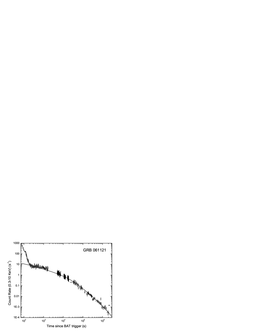
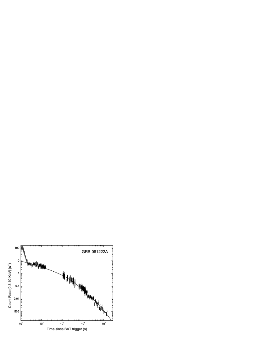
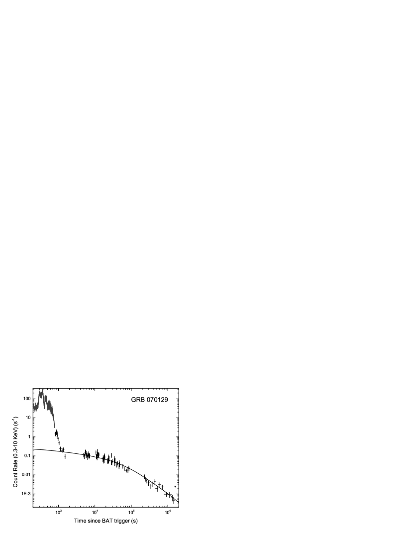
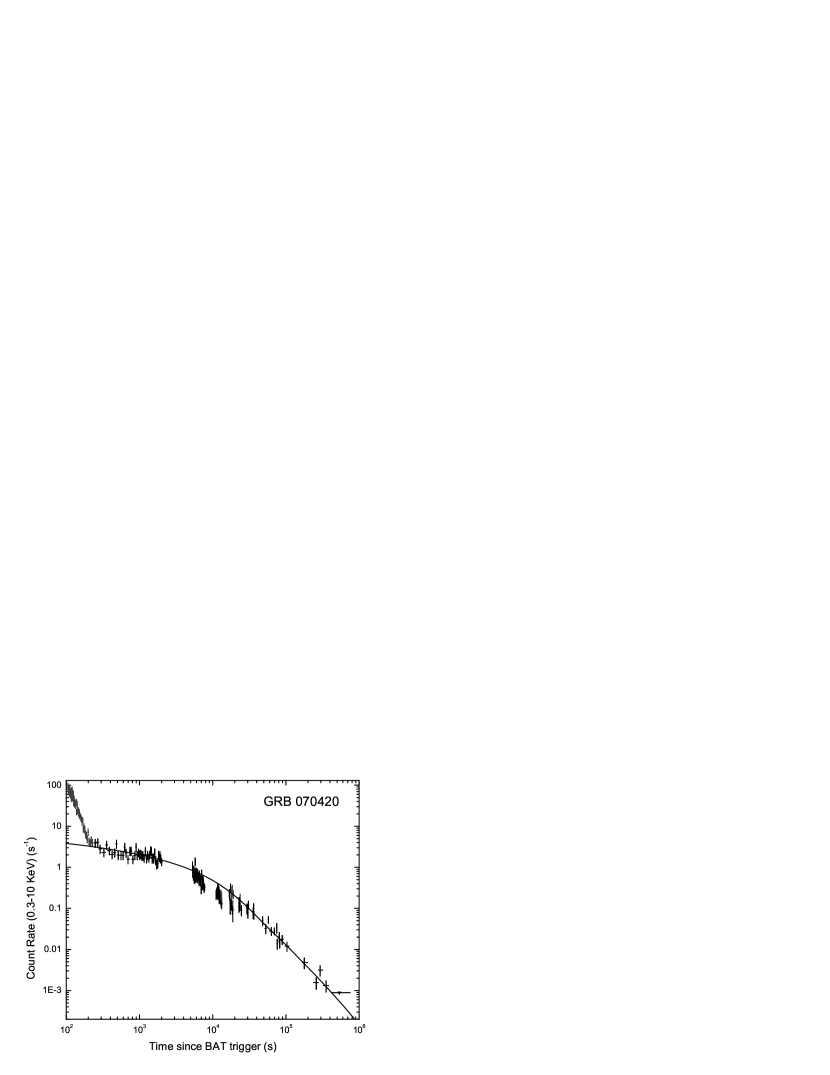
Figure 2: The X-ray light curves of 36 GRBs observed by Swift XRT. WT mode is in gray, PC mode is in black. The solid lines are the theoretical light curves given by our model (Eq. 4). We have $E_{-}=0.3$ keV and $E_{+}=10$ keV for Swift XRT, and we assume $a_{-}=0.005\,\micron$, $\delta=0$, $E_{\rm p}=200$ keV. The other parameters, $s$, $q$, $a_{+}$, and $R$ are given in Tab. 1 and Tab. 2.

Well-monitored X-ray light curves of 36 GRBs (see Fig. 2) were fitted by our theoretical model above (see Eq. 4), using the online data by Evans et al. (2007). A total of 14 events have known redshifts (see Tab. 1) while 22 without known redshifts are fixed to be at $z=1$ (see Tab. 2). We assume $E_{-}=0.3$ keV and $E_{+}=10$ keV for Swift XRT (Gehrels et al., 2004; Evans et al., 2007), $a_{-}=0.005\,\micron$ (Mathis et al., 1977), $\delta=0$, and $E_{\rm p}=200$ keV (Preece et al., 2000). The other parameters, $s$, $q$, $a_{+}$, and $R$ are given in Tab. 1 and Tab. 2. Apparently, $a_{+}$ is almost a constant here (i.e., $a_{+}=0.25\,\micron$, except $a_{+}=0.5\,\micron$ for GRB 050505) and consistent with most results from optical observations (Mathis et al., 1977; Predehl & Schmitt, 1995).

Here $A$ is a numerical coefficient, which is equal to 2$A_{1}A_{2}$ as shown in the Appendix. $A_{1}$ is the coefficient in the integrated GRB spectrum between 0.3 and 10 keV, which is not available based on current working frequency of BAT onboard Swift. Similarly, $A_{2}$ is hardly determined by current observations about the X-ray optical depth. A further analysis of the parameter $A_{1}$ and $A_{2}$ is required once the relevant observational data are sufficient.

In Fig. 2, all the light curves approach to a steep decay ($\propto t^{-2}$), which is already predicted by Eq. (4). Since this is a double integral about $E$ and $a$, $t$ is an independent parameter. Approximately, when $x[\alpha(t)]\gg 1$, we have

$$F^{\rm echo}(t) \propto F_{E,a}^{\rm echo}(t)$$ (10)

$$\propto \left\{{\sin x[\alpha(t)]\over x^{2}[\alpha(t)]}-{\cos x[\alpha(t)]\over x[\alpha(t)]}\right\}^{2}{1\over t}$$

$$\propto {\cos^{2}x[\alpha(t)]\over x^{2}[\alpha(t)]t}$$

$$\propto t^{-2},$$

where $\cos^{2}x[\alpha(t)]$ is a high-frequency periodic function of $t$ when $x[\alpha(t)]\gg 1$, and will be independent on $t$ after the integration over $E$ and $a$. Therefore, letting $x[\alpha(t)]=1$, we have a critical time

$$t_{\rm c} = {h^{2}cR\over 8\pi^{2}(1+z)a^{2}E^{2}}$$ (11)

$$= 10^{4}s\left({2\over 1+z}\right)\left(a\over 0.1\micron\right)^{-2}\left({E}\over 1{\rm keV}\right)^{-2}\left({R\over 100{\rm pc}}\right),$$

after which, the light curves will be approaching the steep decay ($\propto t^{-2}$).

By fitting the light curves, we can indirectly derive the distant $R$ for a given event at redshift $z$ (see Table 1). These values of $R$ appear to be consistent with the observed radii of wind bubbles around WC stars (Marston, 1997; Chu et al., 1999). For bursts without known redshifts we only list a pesudo value of the bubble radius $R_{\rm pseudo}$ assuming a fixed redshift $z=1$ (see Table 2). The larger scatter in $R_{\rm pseudo}$ values for the latter group appears to be a direct consequence of the arbitrary $z=1$ prescription.

5 DISCUSSION AND CONCLUSIONS

Recently, Liang et al. (2007a) provided a comprehensive analysis of shallow decays and “normal” decay segments in GRBs. They concluded in their sample that most GRBs in these two segments have a spectral index $\beta$ around $-1.1$ (as the flux density $F_{E}\propto E^{\beta}$). Here we can also get a knowledge of the spectrum of echo emission based on our analysis (see Eq. A9). Approximately, when $x[\alpha(t)]\simeq\pi$ at a given time $t_{\pi}$, we have

$$F_{E}^{\rm echo}(t_{\pi}) \propto F_{E,a}^{\rm echo}(t_{\pi})$$ (12)

$$\propto S(E)\tau(E,a)$$

$$\propto E^{\delta-s}\,,$$

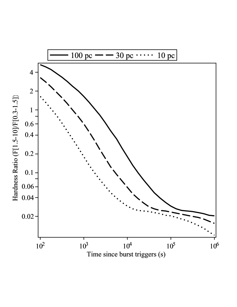
Figure 3: Evolution of the hardness ratio of echo emission with different shell distance $R$. We assume $z=1$, $q=3.5$ and $a_{+}=0.025\,\micron$. Other parameters are the same with Fig. 2. The dramatically small ratio could be alleviated only if the absorption in 0.3-1.5 keV is considered.

where $t_{\pi}$ is about an order of magnitude larger than $t_{\rm d}$ in Eq. (11), and roughly equals most of the $t_{2}$’s defined in Liang et al. (2007a). Therefore, we should have the spectral index $\beta\gtrsim\delta-s$ before $t_{\pi}$, since the spectrum of echo emission is softening in the long run. As shown in Fig. 3, the hardness ratio of echo emission is monotonously decreasing. Interestingly, it reaches a platform (instead of an extremum proposed by Klose, 1998) almost around $t_{\pi}$ and then keeps decreasing very slowly. If we assume $\delta\simeq 0$ (Preece et al., 2000) and $s\sim 2$ (Mauche & Gorenstein, 1986; Mészáros & Gruzinov, 2000), we should have $\beta\gtrsim-2$. This seems to be inconsistent with the observational result by Liang et al. (2007a), since they ended up with $\beta\sim-1.1$.

However, we have two reasons that lead us to be content with our result based on current analysis. First, since we are dealing with the prompt X-ray emission and the $\delta\simeq 0$ here is the result from hard X-rays by BATSE (Preece et al., 2000), we can imagine that the real average $\delta$ should be larger than 0. Specifically, based on the standard synchrotron emission, $\delta$ should equal $1/3$, and the synchrotron self-absorption leads to $\delta\sim 2$. Second, the Rayleigh-Gans approximation is adopted here to calculate the differential cross section of scattering. This approximation overestimates the echo emission at softer X-ray band (say, in 0.3-1.5 keV), where absorption is important, which will change the spectral shape in soft X-ray band and alleviate the dilemma of a dramatically small hardness ratio in Fig. 3. Based on the current analysis, it is safe to say that -2 is only a lower limit for $\beta$. Therefore, our result here is generally consistent with the observations. Thus, the echo emission cannot be completely ruled out for the reason as discussed by Liang et al. (2007a).

Originally, the optical echo emission was used to explain the red bumps observed in some optical afterglows (Esin & Blandford, 2000). However, since the typical optical/infrared scattering angle would be about $\alpha\sim 60\arcdeg$ (White, 1979), the timescale in Eq.(3) would be longer, and the optical/infrared echo emission would be much weaker, and hard to be detected (Reichart, 2001; Heng et al., 2007). Nevertheless, if the WR wind within a much shorter distance ($R\sim 10^{14}-10^{15}$ cm) is also taken into account, there might be detectable variations in the optical afterglows due to echo emission (Moran & Reichart, 2005). However, the average LBV or WR wind bubble around a massive star at its death would be much larger (García-Segura & Mac Low, 1995a, b). Therefore, the features of echo emission in the optical band would be not significant enough, which is possibly the reason that the standard external shock model was more successful in the pre-Swift era, when the optical observations dominated.

Furthermore, the dramatic variations in the LBV or/and WR winds would drive instabilities that produce radial filaments in the LBV or WR shells (García-Segura et al., 1996a, b; Dwarkadas, 2007), which could be the origin of some flares in the X-rays afterglows (Burrows et al., 2006). Therefore, there might be another timescale due to the angular variation of these filaments, which could be given by

$$t_{\rm f} = {(1+z)R_{\rm f}\alpha_{\rm f}^{2}\over 2c},$$ (13)

where $R_{\rm f}$ is the distance of the filaments from the progenitor and $\alpha_{\rm f}$ is the typical angular size of the clumps and ripples in the filaments. To account for the mean ratio of the width and peak time of the X-ray flares (Burrows et al., 2007; Chincarini et al., 2007), i.e., $t_{\rm f}/t_{\rm d}\sim<\Delta t/t>\sim 0.1$, we may have $\alpha_{\rm f}\sim 0.1\,\alpha\sim 0.1\arcmin$.

Sazonov & Sunyaev (2003) claimed on a different scattering circumstance (molecular and atomic matter instead of dust grains) that the opening angle of jets might be an important factor to the echo light curve, based on the popular assumption that the GRB prompt emission is beamed. Since only small-angle scattering ($\alpha\sim 1\arcmin$) for dust grains is considered here, the typical jet properly pointing at us with a much larger opening angle of about few degrees will not affect out results. However, the GRB jet might be pointing at us with its edge in some case, where our result here would not be valid. Instead, a rapid drop that is much steeper than $t^{-2}$ will emerge at a late time (Sazonov & Sunyaev, 2003). This is probably the case for some GRBs, e.g., GRB 060526 (Dai et al., 2007).

In this paper, we have presented the X-ray echo emission in GRB phenomenon and we can draw the following conclusions:

1. The shallow decay phase can still be understood without additional contributions from the central engine (Zhang et al., 2006; Liang et al., 2007a). Interestingly, the feature of a shallow decay followed by a “normal” decay and a further rapid decay can be reproduced by the echo from the prompt X-ray emission scattered by the massive wind bubble around the progenitor (García-Segura et al., 1996a; Mirabal et al., 2003; Dwarkadas, 2007). In general, dust formation seems to be prevailing in carbon-rich WR stars of the WC subtype and there is where echo emission would be most efficient.

2. Echo emission can be an additional X-ray source that masked the X-ray jet breaks (Sato et al., 2007). Therefore, the lack of jet breaks (Panaitescu et al., 2006; Burrows & Racusin, 2007; Panaitescu, 2007; Liang et al., 2007b) might also be understood via competing echo emission. In addition, some results in the pre-Swift era, say, some correlations relevant for optical breaks might still be valid (Frail et al., 2001; Ghirlanda et al., 2004; Liang & Zhang, 2005) .

3. There is an extra temporal break in X-ray echo emission introduced by $t_{\rm c}$ above. By fitting the light curves, we can indirectly measure the locations of the massive wind bubbles, which will bring us closer to finding the mass loss rate, wind velocity, and the age of the progenitors prior to the GRB explosions (García-Segura et al., 1996a; Dwarkadas, 2007).

4. Even though some features in X-ray afterglows would be better understood if the echo emission is taken into account, the external shock model is still the dominant scenario for optical/infrared afterglows, since echo emission is negligible in the later. In addition, the echo emission model does not completely rule out other interpretations (energy injection, etc.) in the framework of the fireball-shock model. Technically, echo emission takes place at a distance of $\sim$ tens of parsecs, while the internal or/and external shocks are believed to take place within a distance of $\sim 10^{17}$ cm. It is more likely that both of them are taking place in the X-ray afterglow, which potentially complicates the light curves. However, this may raise the problem about GRB radiative efficiencies again. Even by assuming that the X-ray emission is the forward shock emission, the GRB efficiency is already too high to be accommodated by the leading internal shock models (Zhang et al., 2007, and references therein). Assuming an echo-dominated X-ray emission would exacerbate the situation.

Appendix A APPENDIX: DERIVATION OF THE THEORETICAL LIGHT CURVE

The single-scattering approximation is adopted, which is valid up to a scattering optical depth, $\tau_{\rm sca}$, of $\sim$0.5 at 1 keV (Predehl & Klose, 1996; Klose, 1998). Therefore, the echo intensity at the Earth per unit photon energy per unit size of the grains is (see Fig. 1 of Shao and Dai, 2007, for the geometry and quantities defined in this Appendix)

$$I_{E,a}^{\rm echo}(\theta,\phi;t) = F_{E}[t-t_{\rm d}(\theta)]\tau_{a}(E){{\rm d}\sigma\over\sigma_{\rm sca}{\rm d}\Omega},$$ (A1)

where $F_{E}[t-t_{\rm d}(\theta)]$ is the flux density of the initial GRB before a time delay $t_{\rm d}(\theta)$, which is also dependent on the viewing angle $\theta$, $\tau_{a}(E)$ is the frequency-dependent scattering optical depth per unit size of the grains, and the last term is the fraction of the scattered photons, which go into the line of sight in a unit solid angle. The zero time point is set as the trigger of a GRB on the Earth. $\phi$ is the azimuthal angle along the line of sight.

Since the initial GRB is usually much shorter than the long-term afterglow, we can approximate the initial GRB light curve as a pulse. We also assume that the initial GRB spectrum is given by a Band spectrum in the X-ray band (Band et al., 1993), so we have

$$F_{E}[t-t_{\rm d}(\theta)] = A_{1}\left({E\over{100\,{\rm keV}}}\right)^{\delta}{\rm exp}\left[-{(\delta+1)E\over E_{\rm p}}\right]\times\delta[t-t_{\rm d}(\theta)],$$ (A2)

where we only need the segment of the Band spectrum in the lower energy band. $A_{1}$ is a constant, and the time delay from a certain viewing angle $\theta$ is given by (Miralda-Escudé, 1999)

$$t_{\rm d}(\theta)={(1+z)D_{\rm d}D_{\rm s}\theta^{2}\over{2cD_{\rm ds}}}\,.$$ (A3)

Here the Dirac delta function of $t$ can be translated into a function of $\theta$, using the special properties of its own,

$$\delta[t-t_{\rm d}(\theta)]={cD_{\rm ds}\over(1+z)D_{\rm d}D_{\rm s}\theta}\delta[\theta-\hat{\theta}(t)],$$ (A4)

where the function $\hat{\theta}(t)$ is defined as $\hat{\theta}(t)\equiv[2ctD_{\rm ds}/(1+z)D_{\rm d}D_{\rm s}]^{1/2}$ (see the Appendix of Shao and Dai, 2007).

We also assume the frequency-dependent scattering optical depth per unit size of the grains is

$$\tau_{a}(E) = A_{2}\left[{(1+z)E\over{1\,{\rm keV}}}\right]^{-s}\left({a\over 0.1\,\micron}\right)^{4-q},$$ (A5)

where $A_{2}$ is a constant with a dimension of $[a^{-1}]$. This is valid only in a range of the size of the grains, say, $a\in[a_{-},a_{+}]$ (Shao and Dai, 2007, and the references therein).

For the last term in Eq. (A1), we have $d\Omega=\theta{\rm d}\theta{\rm d}\phi$, since $\theta$ is very small. We can do some rearrangement

$${{\rm d}\sigma\over\sigma_{\rm sca}{\rm d}\Omega} = {{\rm d}\sigma\over\sigma_{\rm sca}{\rm d}\Omega_{\rm SC}}{{\rm d}\Omega_{\rm SC}\over{\rm d}\Omega},$$ (A6)

where $\sigma_{\rm sca}$ is the total scattering cross-section, ${\rm d}\Omega_{\rm SC}=\alpha{\rm d}\alpha{\rm d}\phi$ is defined since $\alpha$ is also very small, and we have $\alpha=(D_{\rm s}/D_{\rm ds})\theta$ in geometry. Neglecting the chemical composition or shape of the grains, the Rayleigh-Gans approximation is valid for the differential cross-section (Overbeck, 1965; Alcock & Hatchett, 1978)

$${{\rm d}\sigma\over\sigma_{\rm sca}{\rm d}\Omega_{\rm SC}} = {2\over\pi\ }{j_{1}^{2}(x)\over\alpha^{2}},$$ (A7)

where $x\equiv 2\pi(1+z)aE\alpha/hc$, and $j_{1}(x)=({\rm sin}\,x)/x^{2}-({\rm cos}\,x)/x$ is the first-order spherical Bessel function.

Since the wind bubble is very close to the GRB, we have $D_{\rm s}\simeq D_{\rm d}$ and $D_{\rm ds}\equiv R$. Therefore, the echo flux density at the Earth per unit size of the grains is

$$F_{E,a}^{\rm echo}(t) = \int I_{E,a}^{\rm echo}(\theta,\phi;t){\rm cos}\,\theta{\rm d}\Omega$$ (A8)

$$= AS(E)\tau(E,a)j_{1}^{2}\{x[\alpha(t)]\}{1\over t},$$

where A is a numerical constant, and $S(E)$, $\tau(E,a)$, $j_{1}(x)$, $x(\alpha)$, and $\alpha(t)$ are given by Eqs. (5)-(9). So, the flux density and the flux of echo emission at Earth will be

$$F_{E}^{\rm echo}(t) = \int_{a_{-}}^{a_{+}}F_{E,a}^{\rm echo}(t){\rm d}a$$ (A9)

and

$$F^{\rm echo}(t) = \int_{E_{-}}^{E_{+}}F_{E}^{\rm echo}(t){\rm d}E\,,$$ (A10)

respectively.

Table 1: Model parameters of 14 GRBs with known redshifts.

GRB	z	Begin (s)	End (s)	s	q	$a_{+}(\micron)$	$R$(pc)	$\chi^{2}/{\rm dof}$
GRB 050319	3.240	$4\times 10^{2}$	$2\times 10^{6}$	2.5	4.4	0.25	75	1.72
GRB 050505	4.27	$3\times 10^{3}$	$2\times 10^{6}$	2.0	4.0	0.5	50	1.42
GRB 050814	5.3	$1\times 10^{3}$	$1\times 10^{6}$	3.0	4.5	0.25	55	3.53
GRB 051022	0.8	$1\times 10^{4}$	$1\times 10^{6}$	2.0	3.1	0.25	30	2.85
GRB 060210	3.91	$3\times 10^{3}$	$8\times 10^{5}$	2.0	3.0	0.25	200	1.78
GRB 060218	0.033	$1\times 10^{4}$	$1\times 10^{6}$	3.0	3.1	0.25	50	1.92
GRB 060502A	1.51	$4\times 10^{3}$	$2\times 10^{6}$	3.0	4.3	0.25	65	1.26
GRB 060512	0.4428	$3\times 10^{3}$	$3\times 10^{5}$	2.0	3.0	0.25	45	2.63
GRB 060707	3.425	$1\times 10^{3}$	$2\times 10^{6}$	3.0	4.5	0.25	170	2.53
GRB 060714	2.711	$3\times 10^{2}$	$1\times 10^{6}$	2.0	4.0	0.25	95	2.61
GRB 060814	0.84	$8\times 10^{2}$	$1\times 10^{6}$	2.0	4.0	0.25	34	2.33
GRB 060729	0.54	$5\times 10^{2}$	$1\times 10^{7}$	3.0	5.5	0.25	45	2.93
GRB 061110A	0.758	$6\times 10^{3}$	$7\times 10^{5}$	3.0	4.5	0.25	76	2.61
GRB 061121	1.314	$2\times 10^{2}$	$2\times 10^{6}$	2.0	4.0	0.25	40	2.30

Table 2: Model parameters of 22 GRBs without known redshifts

GRB	Begin (s)	End (s)	s	q	$a_{+}(\micron)$	$R_{\rm pseudo}$ (pc)	$\chi^{2}/{\rm dof}$
GRB 050712	$4\times 10^{3}$	$2\times 10^{6}$	2.3	4.3	0.25	55	2.75
GRB 050713A	$4\times 10^{3}$	$2\times 10^{6}$	2.0	4.0	0.25	45	2.67
GRB 050713B	$5\times 10^{2}$	$1\times 10^{6}$	3.0	4.5	0.25	70	2.21
GRB 050802	$3\times 10^{2}$	$1\times 10^{6}$	2.0	3.1	0.25	30	4.64
GRB 050822	$1\times 10^{3}$	$5\times 10^{6}$	3.0	4.5	0.25	80	2.19
GRB 050915B	$1\times 10^{3}$	$5\times 10^{5}$	3.0	4.8	0.25	70	1.60
GRB 051008	$3\times 10^{3}$	$4\times 10^{5}$	2.5	3.5	0.25	10	1.93
GRB 051016A	$4\times 10^{3}$	$6\times 10^{5}$	2.3	4.0	0.25	80	6.44
GRB 060204B	$4\times 10^{2}$	$4\times 10^{5}$	2.0	3.1	0.25	25	1.64
GRB 060219	$2\times 10^{2}$	$4\times 10^{5}$	2.5	3.5	0.25	45	1.04
GRB 060306	$3\times 10^{2}$	$3\times 10^{5}$	2.0	4.0	0.25	50	1.41
GRB 060428A	$3\times 10^{2}$	$3\times 10^{6}$	2.7	4.2	0.25	95	2.26
GRB 060510A	$1\times 10^{2}$	$5\times 10^{5}$	3.0	4.5	0.25	10	2.28
GRB 060604	$3\times 10^{3}$	$1\times 10^{6}$	2.0	4.0	0.25	80	1.86
GRB 060708	$2\times 10^{2}$	$1\times 10^{6}$	2.0	4.0	0.25	50	2.03
GRB 060813	$9\times 10^{1}$	$2\times 10^{5}$	2.0	3.1	0.25	10	2.68
GRB 061004	$3\times 10^{2}$	$1\times 10^{5}$	2.0	4.0	0.25	15	2.61
GRB 061222A	$2\times 10^{2}$	$2\times 10^{6}$	2.1	4.2	0.25	30	1.90
GRB 070129	$1\times 10^{3}$	$2\times 10^{6}$	3.0	4.5	0.25	90	1.63
GRB 070328	$1\times 10^{2}$	$6\times 10^{5}$	1.9	4.0	0.25	5	4.75
GRB 070419B	$4\times 10^{3}$	$4\times 10^{5}$	2.0	3.1	0.25	20	2.74
GRB 070420	$3\times 10^{2}$	$4\times 10^{5}$	3.0	3.1	0.25	15	3.07

References

- Alcock & Hatchett (1978) Alcock, C., & Hatchett, s. 1978, ApJ, 222, 456
- Allen et al. (1972) Allen, D. A., Harvey, P. M., & Swings, J. P. 1972, A&A, 20, 333
- Band et al. (1993) Band, D. L. et al. 1993, ApJ, 413, 281
- Burrows & Racusin (2007) Burrows, D. N., & Racusin, J. 2007, Procs. of the “Swfit and GRBs: Unveiling the Relativistic Universe” Conf., Venice (astro-ph/0702633)
- Burrows et al. (2007) Burrows, D. N., et al. 2007, Philosophical Transactions A, in press (astro-ph/0701046)
- Burrows et al. (2006) Burrows, D. N., et al. 2006, Proceedings of the X-Ray Universe Conference, (ESA SP-604; Noordwijk: ESA), 877
- Castor et al. (1975) Castor, J., McCray, R., & Weaver R. 1975, ApJ, 200, L107
- Chincarini et al. (2007) Chincarini, G., et al. 2007, ApJ, in press (astro-ph/0702371)
- Chu et al. (1999) Chu, Y.-H., Weis, K., & Garnett, D. R. 1999, AJ, 117, 1433
- Costa (1999) Costa, E. 1999, A&AS, 138, 425
- Crowther (2007) Crowther, P. A. 2003, ARA&A, 45, 177
- Crowther (2003) Crowther, P. A. 2003, Ap&SS, 285, 677
- Dai et al. (2007) Dai, X., et al. 2007, ApJ, 658, 509
- Dai (2004) Dai, Z. G. 2004, ApJ, 606, 1000
- Dai & Lu (1998) Dai, Z. G., & Lu, T. 1998, A&A, 333, L87
- Dwarkadas (2007) Dwarkadas, V. V. 2007, ApJ, 667, 226
- Evans et al. (2007) Evans, P. A., et al. 2007, A&A,469, 379
- Esin & Blandford (2000) Esin, A. A., & Blandford, R. D. 2000, ApJ, 534, L151
- Fan & Piran (2006) Fan, Y. Z., & Piran T. 2006, MNRAS, 369, 197
- Frail et al. (2001) Frail, D. A., et al. 2001, ApJ, 562, L55
- García-Segura & Mac Low (1995a) García-Segura, G., & Mac Low, M. M. 1995a, ApJ, 455, 145
- García-Segura & Mac Low (1995b) García-Segura, G., & Mac Low, M. M. 1995b, ApJ, 455, 160
- García-Segura et al. (1996a) García-Segura, G., et al. 1996a, A&A, 305, 229
- García-Segura et al. (1996b) García-Segura, G., et al. 1996b, A&A, 316, 133
- Gehrels et al. (2004) Gehrels, N., et al. 2004, ApJ, 611, 1005
- Gehrz & Hackwell (1974) Gehrz, R. D., & Hackwell, J. A. 1974, ApJ, 194, 619
- Ghirlanda et al. (2004) Ghirlanda, G., et al. 2004, ApJ, 616, 331
- Heng et al. (2007) Heng, K., Lazzati, D., & Perna, R. 2007, ApJ, 662, 1119
- Klose (1998) Klose, S. 1998, ApJ, 507, 300
- Langer et al. (1994) Langer, N., et al. 1994, A&A, 290, 819
- Liang et al. (2007a) Liang, E. W., Zhang, B. B., & Zhang, B. 2007a, ApJ, in press (arXiv: 0704.1373)
- Liang et al. (2007b) Liang, E. W., et al. 2007b, ApJ, submitted (arXiv: 0708.2942)
- Liang & Zhang (2005) Liang, E. W., & Zhang, B. 2005, ApJ, 633, 611
- Marston (1997) Marston, A. P. 1997, ApJ, 475, 188
- Mathis et al. (1977) Mathis, J. S., Rumpl, W., & Nordsieck, K. H. 1977, ApJ, 217, 425
- Mauche & Gorenstein (1986) Mauche, C. W., & Gorenstein, P. 1986, ApJ, 302, 371
- Mészáros & Gruzinov (2000) Mészáros, P., & Gruzinov, A. 2000, ApJ, 543, L35
- Mészáros (2006) Mészáros, P. 2006, Rep. Prog. Phys., 69, 2259
- Mirabal et al. (2003) Mirabal, N., et al. 2003, ApJ, 595, 935
- Miralda-Escudé (1999) Miralda-Escudé, J. 1999, ApJ, 512, 21
- Moran & Reichart (2005) Moran, J. A., & Reichart, D. E. 2005, ApJ, 632, 438
- Nousek et al. (2006) Nousek, J. A., et al. 2006, ApJ, 642, 389
- Overbeck (1965) Overbeck, J. W. 1965, ApJ, 141, 864
- Panaitescu et al. (2006) Panaitescu, A., et al. 2006, MNRAS, 369, 2059
- Panaitescu (2007) Panaitescu, A. 2007, MNRAS, 380, 374
- Predehl & Klose (1996) Predehl, P., & Klose, S. 1996, A&A, 306, 283
- Predehl & Schmitt (1995) Predehl, P., & Schmitt, J. H. M. M. 1995, A&A, 293, 889
- Preece et al. (2000) Preece, R. D., et al. 2000, ApJS, 126, 19
- Ramirez-Ruiz et al. (2001) Ramirez-Ruiz, E., et al. 2001, MNRAS, 327, 829
- Rees & Mészáros (1998) Rees, M., & Mészáros, P. 1998, ApJ, 496, L1
- Reichart (2001) Reichart, D. E. 2001, ApJ, 554, 643
- Rhoads (1999) Rhoads, J. E. 1999, ApJ, 525, 737
- Sari & Mészáros (2000) Sari, R., & Mészáros, P. 2000, ApJ, 535, L33
- Sakamoto et al. (2007) Sakamoto, T., et al. 2007, ApJS, in press (arXiv: 0707.4626)
- Sato et al. (2007) Sato, G., et al. 2007, ApJ, 657, 359
- Sazonov & Sunyaev (2003) Sazonov, S. Y., & Sunyaev, R. A. 2003, A&A, 399, 505
- Shao and Dai (2007) Shao, L., & Dai, Z. G. 2007, ApJ, 660, 1319
- White (1979) White, R. L. 1979, ApJ, 229, 954
- Williams et al. (1987) Williams, P. M., van der Hucht, K. A., & Thé, P. S. 1987, A&A, 182, 91
- Woosley & Bloom (2006) Woosley, S. E., & Bloom, J. S. 2006, ARA&A, 44, 507
- Zhang (2007) Zhang, B. 2007, ChJAA, 7, 1
- Zhang et al. (2007) Zhang, B., et al. 2007, ApJ, 655, 989
- Zhang et al. (2006) Zhang, B., et al. 2006, ApJ, 642, 354
- Zhang, & Mészáros (2001) Zhang, B., & Mészáros, P. 2001, ApJ, 552, L35