Homogeneous nucleation of dislocations as bifurcations in a periodized discrete elasticity model

Abstract

A novel analysis of homogeneous nucleation of dislocations in sheared two-dimensional crystals described by periodized discrete elasticity models is presented. When the crystal is sheared beyond a critical strain $F=F_{c}$, the strained dislocation-free state becomes unstable via a subcritical pitchfork bifurcation. Selecting a fixed final applied strain $F_{f}>F_{c}$, different simultaneously stable stationary configurations containing two or four edge dislocations may be reached by setting $F=F_{f}t/t_{r}$ during different time intervals $t_{r}$. At a characteristic time after $t_{r}$, one or two dipoles are nucleated, split, and the resulting two edge dislocations move in opposite directions to the sample boundary. Numerical continuation shows how configurations with different numbers of edge dislocation pairs emerge as bifurcations from the dislocation-free state.

1 Introduction

Homogeneous nucleation of dislocations is observed in different processes such as nanoindentation experiments [1, 2], heteroepitaxial crystal growth [3, 4], indentation experiments in colloidal crystals [5] or soap bubble raft models [6]. Homogeneous nucleation of dislocations occurs in a perfect crystal and is therefore expected to have a much higher activation energy than heterogeneous nucleation at defect sites such as step edges. Different types of calculations have been used to interpret homogeneous nucleation of dislocations in different situations, ranging from atomistic simulations to continuum mechanics interpretations or combinations thereof [7]. In all cases, a reliable nucleation criterion is needed to capture the nature of nucleated defects and the time and place at which such defects appear.

In this letter, we tackle homogeneous nucleation of dislocations as a bifurcation problem in discrete elasticity. Periodized discrete elasticity models of dislocations regularize in a natural way the singularities of the stress field at the dislocation lines that appear in the theory of elasticity, and they also allow the sliding motion of crystal planes typical of dislocation gliding [8, 9]. Simplified versions of these models have been used to analyze dislocation depinning and motion at the Peierls stress in a precise manner [10]. Here we show that simple periodized discrete elasticity models are able to describe homogeneous nucleation of dislocations by shearing an initially undisturbed dislocation-free lattice. While molecular dynamics produces nucleation of dislocations and the Peierls stress, it is considerably costlier than periodized discrete elasticity. In more efficient computer codes of discrete line dislocation dynamics, nucleation of dislocations and the Peierls stress have to be added to the code [7]. Moreover, simple models allow for a more detailed analysis and interpretation of results than either these computer-intensive methods.

The idea behind periodized discrete elasticity models is to discretize space according to the nodes of the crystal lattice. Then the potential energy of the crystal is constructed as follows. The usual strain energy density of linear elasticity is obtained from the tensor of elastic constants and the strain tensor which is the symmetrized gradient of the displacement vector. In periodized discrete elasticity models of simple cubic crystals, the gradient of the displacement vector is replaced by a periodic function of the finite differences of the displacement vector that has the same period as the lattice and is linear for small differences. The potential energy is obtained from the resulting strain energy density by summing over all lattice points [8]. The equations of motion obtained from the crystal potential energy reduce to those of linear anisotropic elasticity far from the dislocation cores, where the differences of the displacement vector are small and approximately equal to their partial derivatives. At the dislocation cores, the singularities of the stress field are regularized by the lattice and gliding is allowed by the above mentioned periodic functions. Extensions to bcc and fcc crystals [8] or to lattices with a two-atom basis [9] are possible. While these models are three-dimensional, it is possible to simplify them for simple geometrical configurations such as planar edge dislocations having parallel Burgers vectors. In this case, the component of the displacement vector parallel to the Burgers vector suffices to describe depinning and gliding of dislocations. A simplified model retaining only this component has been used to analyze dislocation depinning and motion at the Peierls stress [10]. The same phenomena occur in the same way in the more complete models having two nonzero components of the displacement vector [8].

2 Model

Here we study a simple 2D periodized discrete elasticity scalar model that may describe homogeneous nucleation of edge dislocations with parallel Burgers vectors and is amenable to detailed analysis. Consider a 2D simple cubic lattice with lattice constant normalized to 1, lattice points labelled by indices $(i,j)$, $i=1,...,N_{x}$ and $j=1,...,N_{y}$, and displacement vector $(u_{i,j},0)$. At the boundary, a shear strain $F$ is applied, so that the displacement $u_{i,j}$ for $j=1,N_{y}$ and for $i=1,N_{x}$ is $F\,[j-(N_{y}+1)/2]$. $F$ is also the dimensionless shear stress. To visualize more easily the lattice, we will sometimes use coordinates $(x,y)$ with $x=i-(N_{x}+1)/2$ and $y=j-(N_{y}+1)/2$ centered at the lattice center. In these coordinates, the boundary displacement adopts its usual form $Fy$. $u_{i,j}$ obeys the following nondimensional equations:

$$m{d^{2}u_{i,j}\over dt^{2}}+\alpha{du_{i,j}\over dt}=u_{i+1,j}-2u_{i,j}+u_{i-1,j}$$

$$\quad\quad+A\,[g_{a}(u_{i,j+1}-u_{i,j})+g_{a}(u_{i,j-1}-u_{i,j})].$$ (1)

Here $A=C_{44}/C_{11}$ provided we consider cubic crystals with elastic constants $C_{11}$, $C_{12}$, $C_{44}$. If we select a nondimensional time scale $C_{11}t/(\rho l^{2}\gamma)\to t$, then $\alpha=1$ and $m=C_{11}/(\rho l^{2}\gamma^{2})$, where $\gamma$ is a friction coefficient with units of frequency, $\rho$ is the mass density and $l$ the dimensional lattice constant. The nondimensional displacement vector is measured in units of $l$. With this choice of scales, we can consider the overdamped case with $m=0$. On the other hand, if we select a nondimensional time scale $C_{11}^{1/2}t/(l\rho^{1/2})\to t$, then $m=1$ and $\alpha=l\gamma\sqrt{\rho/C_{11}}$. With this second choice of scales, we can consider the conservative case with $\alpha=0$.

The nonlinear function $g_{a}$ is periodic, with period equal to the lattice space and $g_{a}^{\prime}(0)=1$. It allows gliding of half columns of atoms in the $x$-direction, which is the direction of the Burgers vectors of the edge dislocations that will be nucleated. Gliding along other directions is not possible in this model: we would need a two-component displacement vector and a periodic function of finite differences along the $x$ axis [8]. We have used in our simulations the continuous one-parameter family of periodic functions

$$g_{a}(x)={2a\over\pi}\left\{\begin{array}[]{ll}\sin\left({\pi x\over 2a}\right),&-a\leq x\leq a,\\ \sin\left({\pi(x-1/2)\over 2a-1}\right),&a\leq x\leq 1-a,\\ \end{array}\right.$$ (4)

with $0\leq a\leq 1/2$ and period 1. In the symmetric case $a=1/4$, (1) - (4) is the interacting atomic chains model [11]. The parameter $a$ controls the asymmetry of $g_{a}$, which in turn determines the size of the dislocation core and the Peierls stress needed for a dislocation to start moving [8]. As $a$ increases, the interval over which $g^{\prime}_{a}(x)>0$ increases at the expense of the interval over which the slope of $g_{a}$ is negative. Then as $a$ increases, so does the Peierls stress, whereas both the core size and the mobility of defects decrease. Large values of $a$ result in very narrow cores and large Peierls stresses. The value of $a$ can be selected so that the Peierls stress calculated from (1) fits experimental values or values calculated using molecular dynamics [8].

We consider first the overdamped case, $m=0$, $\alpha=1$ with $A=0.3071$ (corresponding to tungsten), $a=0.2$. In this case and for time independent shear, the potential energy

$$V=\sum_{i,j}\left[{1\over 2}\,(u_{i+1,j}-u_{i,j})^{2}+A\,G_{a}(u_{i+1,j}-u_{i,j})\right],$$ (5)

with $G^{\prime}_{a}(x)=g_{a}(x)$ and $G_{a}(0)=0$ is a Lyapunov functional of the gradient system (1): it satisfies $V\geq 0$ and

$${dV\over dt}=\sum_{i,j}{\partial V\over\partial u_{i,j}}\,{du_{i,j}\over dt}=-\sum_{i,j}\left({du_{i,j}\over dt}\right)^{2}\leq 0,$$

since $du_{i,j}/dt=-\partial V/\partial u_{i,j}$ and the shear strain $F$ does not depend on time. In the unstressed crystal configuration $F=0$, a given initial condition evolves exponentially fast to a stable homogeneous dislocation-free stationary state which we call BR0. This stable solution of the discrete model is simply the undisturbed lattice without any dislocations. As we select larger and larger positive stresses, the homogeneous stationary configuration BR0 is strained but it continues to be stable and dislocation-free until a critical stress $F_{c}=0.2193$ is reached. At $F_{c}$, the maximum eigenvalue of Eq. (1) linearized about the stationary solution BR0 becomes zero. What happens for $F>F_{c}$?

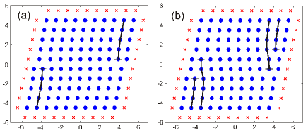
Figure 1: Configurations of the stationary solutions (a) BR1, (b) BR2, at $F_{f}=0.22$. Parameter values are $a=0.2$, $A=0.3071$ for a 10x10 lattice. The crosses represents the positions of the boundary atoms which are fixed by the shear boundary condition.

3 Multistable configurations with dislocations

One way to proceed is to start from the stable stationary configuration BR0 at $F=0$. We then increase the shear strain $F$ to a small value $\Delta F$, use the configuration BR0 for $F=0$ as initial condition, solve (1) and find the corresponding stable stationary configuration. Repeating this procedure, we follow BR0 until $F_{c}$ and for $F>F_{c}$ we obtain the configuration BR2 at the corresponding value of $F$ depicted in Fig. 1(b). The stationary configuration contains four edge dislocations, two with Burgers vector $(1,0)$, the other two with Burgers vectors $(-1,0)$. These dislocations appear as the result of the nucleation of two edge dipole dislocations at $y=\pm 1$. Immediately after they are created, these dipoles split into their component dislocations that move in opposite directions until they reach the sample boundary. Why do dipoles split in opposite moving edge dislocations? The strain needed for a given edge dislocation dipole to split into its component dislocations is about $F_{c}/10$ [12], much smaller than the strain $F_{c}$ needed to nucleate a dipole. Thus the dipoles split into opposite moving dislocations immediately after being created.

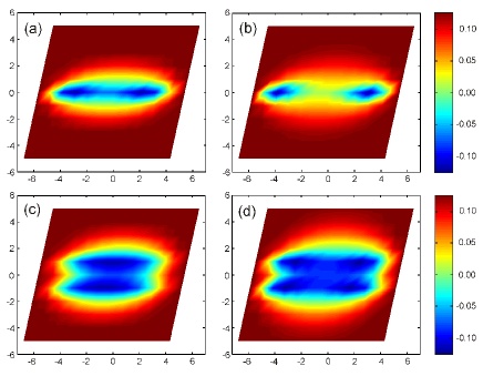
Figure 2: Four snapshots of the strain $2e_{1,2}$ at times (a) 1491.8 and (b) 2643.2 for the evolution towards BR1 at ramping time $t_{r}=86$ ($c_{r}=0.0026$), and at times (c) 2056 and (d) 3242.3 for the evolution towards BR2 at ramping time $t_{r}=1000$ ($c_{r}=2.2\times 10^{-4}$). $F_{f}=0.22$ and other parameter values as in Fig. 1.

Can we obtain other configurations by doing things differently? The answer is yes. Suppose we want to explore the stable stationary configurations at a strain $F_{f}=0.22$ slightly larger than $F_{c}$. Starting with BR0 at $F=0$, we turn in the strain according to a linear law during a time $t_{r}$ (the ramping time) and leave $F=F_{f}$ for $t>t_{r}$. Then $F(t)=c_{r}t\,H(t_{r}-t)+F_{f}H(t-t_{r})$, where $c_{r}=F_{f}/t_{r}$ and $H(x)$ are the strain rate and the Heaviside unit step function, respectively. Same as in other multistable systems [13], we obtain different final stable configurations depending on $F_{f}$ and $t_{r}$. For long ramping times $t_{r}>87$, we again find BR2. Fig. 2(c) and (d) show two snapshots of the strain component $2e_{1,2}=g_{a}(u_{i,j+1}-u_{i,j})$ taken after $F$ has reached its final value $F_{f}$ and $u_{i,j}$ is evolving towards its final stationary configuration. We observe two depressions of the strain $e_{1,2}$ at $y=\pm 1$ indicating nucleation of two dislocation dipoles. As we have said before, the Peierls stress needed to split and move the component dislocations in a dipole is much smaller than the stress required for homogeneous nucleation of one dipole. Thus after being nucleated, the edge dislocations with opposite Burgers vectors comprising each dipole immediately move in opposite directions towards the lattice boundaries. The final configuration is BR2. For shorter ramping times ($82<t_{r}<87$), Figs. 2(a) and (b) show that only one dislocation dipole is nucleated, splits into two edge dislocations with opposite Burgers vectors that then move towards the boundaries in opposite directions. The final configuration is BR1 as in Fig. 1(a). For $t_{r}<81$, a final configuration BR3 (similar to that in Fig 1(b) but not explicitly shown) is reached after two dipoles are nucleated at the upper and lower boundaries and their component dislocations move to the left and right boundaries in opposite directions.

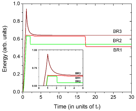
Figure 3: Energy $V(t)$ for ramping times 10 (BR3), 86 (BR1) and 1000 (BR2). Parameter values are the same as in Fig. 1.

4 Nucleation time

Fig. 3 shows the evolution of the potential energy when the same final strain $F_{f}$ is reached at three different strain rates. We observe that for very short ramping times, e.g., $t_{r}=10$, the energy reaches a peak (with strain energy larger than that of the homogeneous branch $V_{\rm BR0}=0.6335$) at $t_{r}$ and then relaxes toward its final value $V_{\rm BR3}=0.6433$ corresponding to configuration BR3. For very long ramping times, $V(t)$ follows BR0 adiabatically beyond $t_{r}$, at the plateau $V=V_{\rm BR0}$ that lasts from $t_{r}$ until $2\,t_{r}$. At this later time, the energy drops abruptly to its final value corresponding to configuration BR2 in Fig. 1(b) with strain energy $V=V_{\rm BR2}=0.5417$. The abrupt energy drop marks the nucleation of the two dipoles. Similarly, the precipitous energy drop in the evolution towards configuration BR1 of Fig. 1(a) with energy $V_{\rm BR1}=0.5143$ corresponds to the nucleation of one dipole after a long plateau with strain energy $V_{\rm BR0}$ ends abruptly at time $17\,t_{r}$. Note that the evolution towards BR1 starts with a small spike at $t=t_{r}$ (for an intermediate ramping time of 86), it continues with energy $V=0.6435$ at a short plateau for times $1<t/t_{r}<2.5$, there is a gradual energy decay to the long plateau at $V_{\rm BR0}=0.6335$ that lasts from $t=3.5\,t_{r}$ till $t=17\,t_{r}$, and then the strain energy drops to its final value $V_{\rm BR1}=0.5143$.

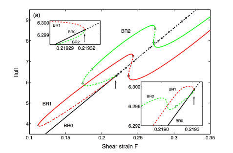
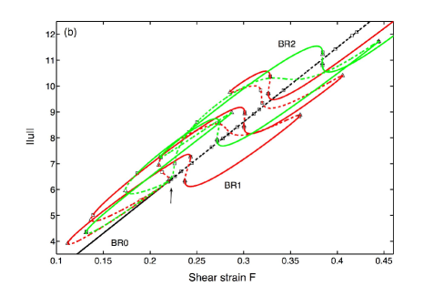
Figure 4: (a) Bifurcation diagram showing only the primary stationary branches issuing from the homogeneous solution BR0. At $F_{c}$, branches BR1 and BR2 appear as a subcritical pitchfork bifurcation from BR0 (see the insets). (b) Larger view of the bifurcation diagram showing branches that are prolongations of BR1 and BR2 after a number of limit and bifurcation points. Solid lines correspond to stable solutions, dashed lines to unstable solutions, limit points are marked as triangles and bifurcation points as squares. Parameter values are the same as in Fig. 1.

5 Bifurcation diagram

More precise information about possible stable configurations can be obtained by examining the bifurcation diagram of the $l^{2}$ norm of the displacement, $||u||=\sqrt{\sum u_{i,j}^{2}}$ (the sum excludes points at the boundaries), versus the strain $F$. The complete bifurcation diagram has been calculated using the AUTO program of numerical continuation of solutions [14], and it is rather complex: there are many bifurcation points issuing from different stationary solution branches, most of which are unstable. If we depict all possible solution branches, the resulting bifurcation diagram is rather messy. Thus we have chosen to depict only important solution branches which are stable in certain strain intervals.

In Fig. 4(a) we show the only two primary branches that bifurcate from BR0 at $F=F_{c}=0.2193$. The inset shows that these branches appear as a subcritical pitchfork bifurcation at $F=F_{c}$. Both start being unstable for $F$ close to $F_{c}$ but become stable after limit points (BR1 exactly after the limit point, BR2 becomes stable after a secondary bifurcation point with $F>F_{l2}$), giving rise to intervals were several stationary solutions are simultaneously stable. As explained before, these configurations can be selected by turning the final shear strain at different rates.

The branches BR1 and BR2 contain a number of secondary bifurcations and limit points, as depicted in Fig. 4(b). These branches fold over themselves in segments delimited by additional limit points and display other linearly stable parts. The configurations thereof contain additional dislocations arising from dipole nucleation. For example, BR1 has another stable configuration at $F_{f}$ arising from nucleation of dipoles at $y=\pm 2$, whereas BR2 has stable configurations arising from dipole nucleation at $y=0,\pm 3$ and at $y=\pm 3$, respectively. While these configurations are linearly stable, we have not been able to reach them by ramping to $F_{f}=0.22$.

It is interesting to note that the strains $2e_{1,2}$ corresponding to the unstable parts of BR1 and BR2 resemble the snapshots corresponding to dipole nucleation in Fig. 2. If we follow the unstable part of BR1 backwards from the limit point at $F_{l1}\approx 0.11$ to the critical strain $F_{c}$, we observe that its strain $2e_{1,2}$ has a depression at x = 0 corresponding to dipole nucleation for $F_{l1}<F<F_{c}$, but this depression becomes less and less observable as we approach $F_{c}$. Similarly, as we follow the unstable part of BR2 from its limit point $F_{l2}\approx 0.17$ to $F_{c}$, we observe that $2e_{1,2}$ first exhibits two symmetric depressions at x = 0 corresponding to nucleation of two dipoles. Then these depressions diminish until the configuration of the unstable part of BR2 becomes very similar to that of BR1 as F approaches $F_{c}$. This is as it should be because BR1 and BR2 merge at $F_{c}$ in a subcritical pitchfork bifurcation: Near $F_{c}$, BR1 and BR2 differ from BR0 by $\propto\pm\sqrt{F_{c}-F}\psi_{i,j}$ ($\psi_{i,j}$ is the eigenvector corresponding to the zero eigenvalue at $F=F_{c}$).

The components of the eigenvector $\psi_{i,j}$ have opposite signs for alternate rows of their corresponding lattice sites, $\psi_{i,j}\psi_{i,j+1}<0$, while they keep the same sign along the same column in the lattice, $\psi_{i,j}\psi_{i,k}>0$. The differences $|\psi_{i,j+1}-\psi_{i,j}|$ are found to be largest at the center of the lattice. We have observed that regions where dislocations may nucleate are located between rows $j$ and $j+1$ for which $\psi_{i,j+1}-\psi_{i,j}$ is maximum ($y=0,\pm 2$ for branch BR1) or minimum ($y=\pm 1,\pm 3$ for branch BR2).

6 Influence of lattice size on bifurcations

In all our figures, we have presented numerical solutions corresponding to a 10x10 lattice, $a=0.2$ and $A=0.3071$. The secondary solution branches (not depicted here) change substantially with $N_{x}$, $N_{y}$, $A$ and $a$. Bifurcation and limit points also might appear or disappear from the diagram. However, BR1 and BR2 persist and the value of $F_{c}$ and the type of the primary bifurcation do not change if we increase the computational domain. For example, $F_{c}=0.2053$ for a 20x20 lattice which is closer to $F_{c}=a$ than the critical strain for a smaller lattice: apparently $F_{c}\to a$ as the lattice size increases. In some cases (small $a$ and small lattices, such as $a=0.1$ in 6x6 and 8x8 lattices), the pitchfork bifurcation at $F_{c}$ is supercritical. However, the bifurcation becomes again subcritical for larger values of $a$ and for larger lattices ($a=0.1$, in 10x10 and 14x14 lattices). Finding the branch BR3 with AUTO has been quite elusive and, in fact, we did not find it for the 10x10 lattice with the parameter values of Fig. 1 using AUTO, whereas ramping produced BR3 in a straightforward manner. For a 6x6 lattice with $a=0.4$, we find that BR3 appears as one of the branches issuing from BR0 as a supercritical pitchfork bifurcation at $F=F_{3}>F_{c}$. This branch has a limit point at a larger strain and it continues for decreasing values of $F$. One of the stretches of BR3 is linearly stable at a range of $F$ overlapping those of BR1 and BR2 [12].

7 Effects of inertia

The bifurcation diagram corresponding to stationary solutions of (1) with inertia ($m\neq 0$) is still the same as presented here. However, the stability character of the solutions changes. In the conservative case $m=1$, $\alpha=0$, stable solutions are no longer asymptotically stable. Linearizing (1) about a stable solution, we find a problem with purely imaginary eigenvalues. Therefore these solutions are centers: small disturbances about them give rise to small permanent oscillations about them. The linearized problem about unstable solutions has pairs of positive and negative eigenvalues and therefore these solutions are saddle-centers in general.

8 Concluding remarks

What have we learned about homogeneous dislocation of nucleations by shearing a dislocation-free state? Clearly the critical strain $F_{c}$ marks the instability of the dislocation-free solution branch BR0. $F_{c}$ is characterized as the shear strain at which the largest eigenvalue of the linear eigenvalue problem about BR0 becomes zero. The components of the corresponding eigenvector indicate possible nucleation sites that are realized by different stationary solution branches in the bifurcation diagram. The fact that the pitchfork bifurcation at $F_{c}$ is subcritical implies that dislocation nucleation can occur at subcritical shear strain values at which the solution branches BR1 and BR2 become stable. Thus it is important to determine the ranges of $F$ at which some of the branches BR0, BR1 and BR2 are simultaneously stable. This cannot be done by simple linear stability calculations: instead numerical continuation algorithms such as AUTO have to be employed. For overdamped dynamics, different stable stationary configurations can be selected by the strain rate at which the final strain $F_{f}$ is reached. An abrupt drop in energy marks the nucleation time at which one or two dipoles are nucleated. Since the Peierls stress is lower than the critical stress for homogeneous dipole nucleation, the dipoles immediately split into edge dislocations with opposite Burgers vectors moving in opposite directions. This bifurcation picture seems to describe larger lattices and it captures the stationary solutions even if inertia is added.

Experimental studies often use ad hoc criteria for nucleation of dislocations such as the critical resolved shear stress (CRSS) [1]. To use this criterion, the critical stress for nucleation has to be related to the applied force by other means, such as the Hertz contact theory in nanoindentation experiments [15, 1]. Moreover, the critical stress itself has to be calibrated independently and it cannot be a fixed value. Instead, the ideal shear stress for nucleation may depend strongly on the other stress components, not just on the shear stress component acting on the plane, as shown by density functional theory [16]. Earlier continuum mechanics studies suggest that nucleation of dislocations is related to the loss of strict convexity in the energy and stress concentration [17]. Recent studies calculate the elastic constants and internal stresses from atomistic calculations or from finite element calculations and the Cauchy-Born hypothesis to figure out atom motion [18]. Then they minimize a certain scalar functional of elastic constants and internal stresses at each point of the solid. Nucleation occurs at those points at which the resulting scalar functional first vanishes [19]. There is a widespread feeling in all these studies that homogeneous nucleation of dislocations is related to some bifurcation occurring once the instability starts but they do not report any precise analysis and calculation of this bifurcation, in contrast to our work.

Dislocation depinning and motion and dislocation interaction occur in the same way in the simple scalar model (1) [10] and in more complete planar discrete elasticity models with two components of the displacement vector [8]. Thus we expect that our bifurcation description of homogeneous nucleation and motion of dislocation dipoles also applies to these planar models. Studies of nucleation of dislocations in more complete two and three dimensional models are postponed to future publications.

- [1] \Name Asenjo A., Jaafar M., Carrasco E. Rojo J.M. \ReviewPhys. Rev. B \Vol73 \Year2006 \Page075431.
- [2] \NameRodríguez de la Fuente O., Zimmerman J. A., González M. A., de la Figuera J., Hamilton J. C., Pai W. W. Rojo J. M. \ReviewPhys. Rev. Lett. \Vol 88 \Year2002 \Page036101.
- [3] \NameBreen K. R., Uppal P. N. Ahearn J. N. \ReviewJ. Vac. Sci. Technol. B \Vol8 \Year1990 \Page730.
- [4] \NameJoyce B. A. Vvedensky D. D. \ReviewMater. Sci. Eng. R \Vol46 \Year2004 \Page127.
- [5] \NameSchall P., Cohen I., Weitz D. Spaepen F. \ReviewNature \Vol440 \Year2006 \Page 319.
- [6] \NameGouldstone A., Van Vliet K. J. Suresh S. \ReviewNature \Vol411 \Year2001 \Page 656.
- [7] \NameBulatov V. V. Cai W. \BookComputer simulations of dislocations \PublOxford University Press, Oxford, UK \Year 2006.
- [8] \NameCarpio A. Bonilla L. L. \ReviewPhys. Rev. B \Vol 71 \Year2005 \Page134105.
- [9] \NameBonilla L. L., Carpio A. Plans I. \ReviewPhysica A \Vol376 \Year2007 \Page361.
- [10] \NameCarpio A. Bonilla L. L. \ReviewPhys. Rev. Lett. \Vol90 \Year2003 \Page135502.
- [11] \NameLandau A. I. \ReviewPhys. stat. sol. (b) \Vol183 \Year1994 \Page407.
- [12] \NamePlans I. \BookDiscrete models of dislocations in crystal lattices: Formulation, analysis and applications. PhD Thesis. \PublUniversidad Carlos III de Madrid \Year2007.
- [13] \NameBonilla L. L., Escobedo R. Dell’Acqua G. \ReviewPhys. Rev. B \Vol73 \Year2006 \Page115341.
- [14] \Name Doedel E. J. et al. AUTO2000, \PublCaltech, Pasadena \Year2001. https://sourceforge.net/projects/auto2000/
- [15] \Name Lorenz D., Zeckzer A., Hilpert U., Grau P., Johansen H. Leipner H. S. \ReviewPhys. Rev. B \Vol 67 \Year2003 \Page 172101.
- [16] \NameOgata S., Li J. Yip S. \ReviewScience \Vol298 \Year2002 \Page807.
- [17] \NameHill R. \ReviewJ. Mech. Phys. Solids \Vol10 \Year1962 \Page1.
- [18] \Name Zhu T., J. Li, Van Vliet K. J., Ogata S., Yip S. Suresh S. \ReviewJ. Mech. Phys. Solids \Vol52 \Year2004 \Page 691.
- [19] \NameLi J., Van Vliet K. J., Zhu T., Yip S. Suresh S. \ReviewNature\Vol418 \Year2002 \Page307.