Data assimilation as a nonlinear dynamical systems problem: Stability and convergence of the prediction-assimilation system

Abstract

We study prediction-assimilation systems, which have become routine in meteorology and oceanography and are rapidly spreading to other areas of the geosciences and of continuum physics. The long-term, nonlinear stability of such a system leads to the uniqueness of its sequentially estimated solutions and is required for the convergence of these solutions to the system’s true, chaotic evolution. The key ideas of our approach are illustrated for a linearized Lorenz system. Stability of two nonlinear prediction-assimilation systems from dynamic meteorology is studied next via the complete spectrum of their Lyapunov exponents; these two systems are governed by a large set of ordinary and of partial differential equations, respectively. The degree of data-induced stabilization is crucial for the performance of such a system. This degree, in turn, depends on two key ingredients: (i) the observational network, either fixed or data-adaptive; and (ii) the assimilation method.

[1]: Institut Royal Météorologique de Belgique, Bruxelles, Belgique^∗

[2]: École Normale Supérieure, Paris, France

[3]: University of California, Los Angeles, CA 90095-1567, USA

[4]: ISAC-CNR, Bologna, Italy

[5]: Novate Milanese, Italy

^∗Corresponding author e-mail: a.carrassi@oma.be

PACS numbers: 05.45.Pq, 02.30.Yy

Physical systems — in nature, the laboratory or industry — can only be measured at a limited number of points in space and time. Estimating the state of a nonlinear dynamical system from partial and noisy observations is therefore crucial in applied physics and engineering [1, 2]. In numerical weather and ocean prediction, this classical estimation problem goes under the name of data assimilation [3, 4]; as data assimilation is spreading rapidly to other fields of the geosciences and of continuum physics, it is important to better grasp its fundamental theoretical aspects. In practice, a data assimilation algorithm has to provide the best-possible estimate of the evolving state of the system, using the observations available and the equations governing the system’s time evolution [5]. In this paper, we examine the long-term stability of the set of modified equations that are referred to as the prediction-assimilation system, in the case in which the original physical system is fully nonlinear and chaotic.

1 Introduction and motivation

1.1 Background

The complete solution of the filtering and prediction problem in sequential-estimation theory [1, 2] is given by the probability density function (PDF) of the unknown state, conditioned on the observations. Given the correct initial PDF and assuming that the system noise and observational noise are white, normally distributed, mutually uncorrelated and known, the PDF’s time evolution can be predicted by the Fokker-Planck equation [1]. In the case of a continuous stochastic dynamical system, with partial observations distributed at discrete times, an ideal data assimilation scheme would solve the Fokker-Planck equation for the time interval between observations and modify the PDF by using all observations when available.

The fundamental difficulty of this approach relates to the high dimension of the state space, which makes it impossible in practice to obtain the initial PDF, let alone compute its time evolution. In the case of linear dynamics and of observations that are linearly related to the system’s state variables, the PDF is fully characterized by its first and second moments, i.e. by the mean and covariance respectively. The optimal solution of the data assimilation problem in this linear setting is provided by the Kalman filter (KF) equations that describe the time evolution of both the mean and the covariance [1, 2, 3, 4, 5, 6, 7]. The time-dependent error-covariance matrix depends, in this linear case, only on the observational error statistics that are part of the problem statement, and not on the actual observations [1].

Thus, in the case of linear dynamics, a linear observation operator, and observational and system noise that are both Gaussian, white in time and mutually uncorrelated, the KF equations give the optimal linear estimate of the state of the system by propagating the associated error covariances, along with the state estimates. In the nonlinear case, the situation is vastly more difficult and the PDF cannot be described by a finite set of parameters. A straightforward way of extending the linear results to the nonlinear case is given by the Extended Kalman filter (EKF) [4, 5, 8, 9].

In the EKF the tangent linear operator is used for predicting the approximate error statistics, while the state evolves according to the full, nonlinear equations. The computational cost of the EKF, though, is still prohibitive in many realistic circumstances. To alleviate this problem, a number of authors have studied reduced-rank approximations of the full EKF [8, 10, 11, 12] that allow a reduction of its computational cost, while maintaining a satisfactory accuracy of the sequential estimates. A Monte Carlo approach, referred to as Ensemble Kalman filter, has also proven effective in reducing the computational cost associated with the full EKF [9, 13, 14].

Early theoretical work on the observability and stability of distributed-parameter systems (i.e., systems governed by coupled partial differential equations) was confined, by-and-large, to linear dynamics and to predetermined observations. In the case of linear, lumped-parameter systems (i.e., systems governed by coupled ordinary differential equations) and observations that are both linear and discrete in time, a sufficient condition for the KF solution to be stable is given by the observability of its dynamics [1, 7]. Cohn and Dee [15] have shown, in the linear, infinite-dimensional case of distributed-parameter systems that it is important to consider observability in the context of the discretized system, and that this observability implies stability of the data-assimilation problem.

The concepts of observability and stability for nonlinear chaotic systems are closely related to other areas of dynamical system theory, namely controlling chaos and synchronization. In the control of chaos, a significant modification of the system’s behavior is achieved by small variations in time of some parameter. Originally devised to stabilize unstable periodic orbits [16], this approach has been generalized to force a given dynamical system to achieve other desiderable types of behavior, wheter stationary, periodic or chaotic [17]. In the present context, synchronization of chaotic systems means essentially using an adaptive coupling to have a ”slaved” system track the motion of a driver or ”master” system [17, 18].

At the core of both chaos control and syncronization lies the stability problem. In the former, the time-dependent control has to be chosen so as to stabilize the motion. In the latter, the stability of the synchronized motion is a necessary condition for achieving such a motion.

Interesting applications of both chaos control and synchronization to geophysical problems include the work of Tziperman et al. [19] on stabilizing an unstable periodic orbit in a fairly realistic El Niño model governed by a set of coupled, nonlinear partial differential equations, as well as that of Duane et al. [20] on meteorological teleconnections between the Atlantic and Pacific sectors of the Northern Hemisphere. Moreover, the relation between synchronization and data assimilation has been investigated by Duane et al. [21] and by Yang et al. [22].

1.2 The present approach

In a chaotic system, initial errors grow within the system’s unstable subspace. Trevisan and Uboldi [23, 24] considered fully nonlinear and possibly chaotic dynamics and proposed, in the context of meteorological data assimilation, to detect and eliminate the unstable components of the forecast error. They showed that those observations that help detect such instabilities maximize error reduction in the state estimates. Ghil [8] and associates (see references there) had already shown that, in meteorological and oceanographic data assimilation, the number of observations necessary to track an unstable flow is comparable to the number of the flow’s dominant degrees of freedom, while Carrassi et al. [25] showed that one can improve on this estimate, since the requisite number of “tracking observations” is closely related to the number and magnitude of the system’s positive Lyapunov exponents.

In this paper, we examine the long-term stability of prediction-assimilation systems. This stability is essential for the performance of data assimilation methods and the convergence of their sequential estimates to the correct evolution of the underlying physical system. We develop a theoretical framework for the study of this long-term stability, and present a theorem that, under certain simplifying assumptions, provides rigorous conditions for the stability of the prediction-assimilation system. Within this framework, we present an approach that optimizes the convergence of the estimates to the correct solution, and apply it to two meteorological models of increasing complexity.

The paper is organized as follows. In Sect. 2 we describe the formulation of data assimilation for nonlinear, chaotic dynamics, with particular emphasis on the proposed approach of Assimilation in the Unstable Subspace (AUS). Section 3 presents first the theorem, its proof and an illustrative numerical example; this illustration is followed by numerical results on the two nonlinear models, one governed by a large system of ordinary differential equations, the other by a system of coupled partial differential equations. Concluding remarks appear in Sect. 4.

2 Data assimilation for chaotic dynamics

We concentrate here on dynamical systems that are perfectly deterministic but chaotic; the role of explicit stochastic forcing, which may represent unresolved scales of motion, will be considered in future work. Without loss of generality, we write the system as a mapping from an arbitrary initial state at time $t_{0}$ to a later time $t$:

$${\bf x}(t)={\cal M}({\bf x}(t_{0})),$$ (1)

where ${\bf x}$ is the $n$-dimensional state vector and ${\cal M}$ the nonlinear evolution operator. Given the initial state ${\bf x}(t_{0})={\bf x}_{0}$, Eq. (1) will predict the state at future times $t$. However, due to the chaotic nature of the system, initial errors will amplify in time, thus setting a limit to the system’s predictability.

The tangent linear equations describing the evolution of infinitesimal perturbations $\delta{\bf x}$ relative to an orbit of Eq. (1) can be written as:

$$\delta{\bf x}(t)={\bf M}\delta{\bf x}(t_{0}),$$ (2)

where ${\bf M}={\bf M}({\bf x}(t_{0}),t-t_{0})$ is the linearized evolution operator associated with ${\cal M}$, along the portion of trajectory between $t_{0}$ and $t$. A chaotic system possesses one or more positive Lyapunov exponents, while their full spectrum characterizes the system’s stability properties; these properties are crucial for the filtering, as well as for the prediction problem [1, 26].

Suppose we seek an estimate of the state of this chaotic dynamical system from a set of noisy observations, given at discrete times $t_{k}\geq t_{0}$, $k\in\{1,2,...\}$,

$${\bf y}^{0}_{k}={\cal H}({\bf x}_{k})+\varepsilon^{o}_{k};$$ (3)

here ${\bf y}^{0}_{k}$ denotes the $p$-dimensional observation vector, ${\bf x}_{k}$ the unknown true state, and $\varepsilon^{o}_{k}$ is the observational error, all at time $t_{k}$, while ${\cal H}$ is the (possibly nonlinear) observation operator. The observational error is assumed to be Gaussian with zero mean and known covariance matrix ${\bf R}$. We consider the underdetermined situation $p\leq n$; typically $p<<n$ in applications.

To obtain an estimate of the state of the system, referred to in meteorological practice as the ${\it analysis}$ ${\bf x}^{a}$, one combines all available observations at $t_{k}$ with the background information, which consists of the forecast state at $t_{k}$. This update is given by the analysis equation:

$${\bf x}^{a}_{k}=({\bf I}-{\bf K}_{k}{\cal H}){\bf x}^{f}_{k}+{\bf K}_{k}{\bf y}^{o}_{k},$$ (4)

where ${\bf x}^{f}_{k}$ indicates the forecast state, and ${\bf K}_{k}$ is the gain matrix at time $t_{k}$. We use here the unified notation [27] for meteorological and oceanographic data assimilation. In most sequential algorithms, the analysis equation has the form (4); such algorithms include the extended Kalman filter (EKF), as well as so-called optimal interpolation and other practical data assimilation schemes [3, 4, 9]. Computing the optimally feasible ${\bf K}$ is at the heart of the sequential-estimation approach to filtering and prediction [1, 2, 6].

The analysis state at time $t_{k}$ is obtained by applying the update (4) at this time to the forecast state ${\bf x}^{f}_{k}$ given by the nonlinear model evolution (1) of the analysis at the previous observation time $t_{k-1}$:

$${\bf x}^{a}_{k}=({\bf I}-{\bf K}_{k}{\cal H}){\cal M}({\bf x}^{a}_{k-1})+{\bf K}_{k}{\bf y}^{o}_{k}.$$ (5)

The repetition of these analysis and forecast steps is referred to as the prediction-assimilation cycle.

The effect of the observations can thus be interpreted as a forcing ${\bf K}({\bf y}^{o}-{\cal H}{\cal M}({\bf x}^{a}))$, which acts on the free solution at the observation times $t_{k}$; note that observations are typically not available at every time step of the discretized set of nonlinear partial differential equations [3, 4]. Equation (5) governs the sequential estimation problem, i.e. the evolving estimate of the state of the system; ${\bf y}^{o}-{\cal H}({\cal M}({\bf x}^{a}))$ here is the innovation vector.

We consider now a perturbed trajectory that undergoes the same forecast and assimilation steps, with the same observations, as the reference trajectory of (5). The equation describing the linear evolution of perturbations $\delta{\bf x}^{f,a}(t_{k})$ of this prediction-assimilation cycle is:

$$\delta{\bf x}^{a}_{k}=({\bf I}-{\bf K}_{k}{\bf H}_{k}){\bf M}_{k-1}\delta{\bf x}^{a}_{k-1},$$ (6)

where ${\bf H}_{k}={\bf H}({\bf x}_{k}^{f})$ is the Jacobian of $\cal H$ at time $t_{k}$ and ${\bf M}_{k-1}$ the linearized evolution operator associated with ${\cal M}$ between $t_{k-1}$ and $t_{k}$. The term $({\bf I}-{\bf K}{\bf H})$ appearing in (6) reflects the effect of the forcing induced by the assimilation. This term modifies the stability properties of the perturbative dynamics relative to (5), i.e. its Lyapunov exponents, with respect to those of the free system (1).

For the updates to drive the solution of Eq. (5) towards the correct solution of Eq. (1), the forecast-assimilation cycle (5) must be stabler than the pure-forecast system (1). Hence the Lyapunov exponents of Eq. (5) must be algebraically smaller than those of Eq. (1), which usually leads to its unstable subspace being lower-dimensional as well. Complete stabilization by the updating process, i.e. total absence of positive Lyapunov exponents, is sufficient for the uniqueness of the solution of Eq. (5), as well as necessary for the convergence of this solution to the true state of the system. Such complete stabilization will drive analysis errors to zero in the absence of observational and system noise, and to the lowest-possible values when noise or nonlinear effects are present.

There are two means at our disposal in order to achieve this stabilization of a prediction-assimilation cycle: the design of the observational network, corresponding to the operator ${\cal H}$, and that of the assimilation scheme, resulting in a certain gain matrix ${\bf K}$; it is the product ${\bf KH}$ in Eq. (6) that provides the stabilizing effect of the forcing by the data. A. Trevisan and associates [23, 24, 25] have proposed an efficient way to achieve this stabilization and improve the performance of the data assimilation method, by monitoring the unstable modes that amplify along a trajectory of the prediction-assimilation system. In their AUS approach, the basis of the subspace to which the analysis update is confined is given by the unstable directions of the system.

The AUS gain matrix K, which differs from zero only on the unstable subspace at an update point, is given by:

$${\bf K}={\bf E}{\bf\Gamma}({\bf HE})^{T}[({\bf HE})\Gamma({\bf HE})^{T}+{\bf R}]^{-1}.$$ (7)

Here ${\bf E}$ is the unitary matrix whose columns are the $m$ unstable directions, while ${\bf\Gamma}$ is a symmetric, positive-definite matrix representing the forecast-error covariance in the subspace spanned by the columns of ${\bf E}$; the index $k$ is omitted in (7) for clarity. Since typically $m<<n$, this feature of the method is clearly efficient in reducing the computational cost of the estimation process. A traditional, fixed network of observations can then be used to detect and reduce the forecast error projection along the unstable directions. An adaptive observational network, designed to measure primarily the unstable modes, will further enhance the efficiency of the assimilation.

The unstable directions of a dynamical system of type (1) can be estimated by the breeding method [28, 29]. In this procedure, the full nonlinear system is used to evolve small perturbations and, at fixed time intervals, their amplitude is scaled down to the initial value. The extension of the breeding technique to Eq. (5), referred to as Breeding on the Data Assimilation System (BDAS) [23], allows one to estimate the unstable directions of a prediction-assimilation system, subject to perturbations that obey Eq. (6). In the AUS assimilation, the unstable directions are used in the definition of the matrix K, cf. Eq. (7), and they can also be used to identify adaptive observations that are most beneficial for error reduction.

3 Results

3.1 Theoretical results

We first provide a theoretical result that, under simplified circumstances, gives the mathematically rigorous condition for the observational forcing to stabilize the prediction-assimilation cycle (5). This result helps to clarify the theoretical underpinnings of AUS. Consider a chaotic flow, with a single positive Lyapunov exponent, and restrict the system’s true evolution to an unstable fixed point, so that $\mathbf{M}$ in Eq. (6) is a constant matrix. The eigenvalues of this matrix are $\Lambda_{i}=e^{(\lambda_{i}\tau)}$, where $\lambda_{i}$ are the Lyapunov exponents, and the eigenvectors of $\mathbf{M}$ are the Lyapunov vectors of the flow, while $\tau=(t_{k}-t_{k-1})$ is the assimilation interval. Alternatively, the result applies to the map associated with integer multiples of the period along an unstable periodic orbit of such a flow.

Let the state of the system be estimated using a single noisy observation at each analysis time, assimilated by AUS along the single unstable direction $\mathbf{e}_{k}$, so that: $\mathbf{K}_{k}=c_{k}\mathbf{e}_{k}$ and $c_{k}=\gamma^{2}\left(\mathbf{He}_{k}\right)\left[\gamma^{2}\left(\mathbf{He}_{k}\right)^{2}+\sigma_{o}^{2}\right]^{-1}$, $\gamma^{2}$ and $\sigma_{o}^{2}$ being the forecast error variance along $\mathbf{e}_{k}$ and the observation error variance, respectively.

Theorem.

Let the constant matrix $\mathbf{M}$ have a single eigenvalue $\Lambda>1$ corresponding to a positive Lyapunov exponent, with $\mathbf{e}$ its associated eigenvector. Let $\mathbf{H}$ be a constant row vector, and the Kalman gain be approximated by $\mathbf{K}_{k}=c\mathbf{e}_{k}$, where $c$ is a constant scalar. The sequence ${\{\bf e}_{k}:k=1,2,...\}$ is defined by the recursion:

$$\Lambda_{k}\mathbf{e}_{k} =\mathbf{Mf}_{k-1},$$ (8a)

$$\Theta_{k}\mathbf{f}_{k} =\left(\mathbf{I}-c\mathbf{e}_{k}\mathbf{H}\right)\mathbf{Mf}_{k-1};$$ (8b)

here the initial $\mathbf{f}_{0}$ is an arbitrarily chosen unit column vector, while $\Lambda_{k}$ and $\Theta_{k}$ are the normalization factors associated with $\mathbf{e}_{k}$ and $\mathbf{f}_{k}$, respectively. Then, a sufficient condition for the solution of (5) to be stable is:

$$c\mathbf{He}>1-{\Lambda}^{-1}.$$

Remark.

The amplitude $c$ of the correction, and the observed (scalar) component $\mathbf{He}$ of the unstable vector, must thus be large enough to counteract the unstable growth.

Proof.

It can be shown that both $\mathbf{e}_{k}$ and $\mathbf{f}_{k}$ converge to $\mathbf{e}$. The range of $\mathbf{K}$ is one-dimensional and the eigenvector $\mathbf{e}$ of $\mathbf{M}$, with associated eigenvalue $\Lambda$, is also an eigenvector of $\left(\mathbf{I}-\mathbf{KH}\right)\mathbf{M}$, with associated eigenvalue $\Theta$

$$\left(\mathbf{I}-c\mathbf{eH}\right)\mathbf{Me}=\left(1-c\mathbf{He}\right)\Lambda\mathbf{e}={\Theta}\mathbf{e}.$$

The stability condition is then obtained by setting $\Theta<1$, and this condition also guarantees uniqueness of the solution. $\quad\square$

To illustrate the essence of the theorem we give here a simple numerical example in the context of the three-variable Lorenz model [30]. When the canonical values of its parameters: $\sigma=10$, $r=28$ and $b=8/3$ are chosen, the system behaves chaotically. In the example that follows, the ”true” state of the system that we want to estimate is the phase-space origin $x=y=z=0$, which is an unstable fixed point for the system. Two assimilation experiments are performed; each one evolves according to the observationally forced, discrete dynamical system (5). At each analysis time a single noisy observation, the $y$-variable, is assimilated.

The time step for integration has been set equal to $0.01$ time units, while the assimilation is performed every $10$ time steps, i.e., $\tau=0.1$ time units; see also Miller et al. [31]. The matrix ${\bf M}$ represents the tangent linear operator evaluated at the origin and integrated for the time interval $\tau$. This matrix possesses exactly one eigenvalue larger than one, $\Lambda=3.26$. The Kalman gain matrix, used to update the analysis, is ${\bf K}_{k}=c{\bf e}_{k}$, with ${\bf e}_{k}$ obtained by the recursive use of Eq. (8). The sequence ${\{\bf e}_{k}\}$ converges to the eigenvector ${\bf e}$ corresponding to the eigenvalue $\Lambda$, and the asymptotic value of ${\bf He}_{k}$ is ${\bf He}=0.91$. The stability condition (9) yields therefore $c>c_{0}=0.762$.

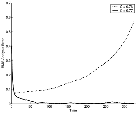
Figure 1: RMS analysis error as a function of time for two experiments with $c=0.76$ and $c=0.77$, below and above the stability threshold $c_{0}=0.762$; the time is given in multiples of the updating interval $\tau=0.1$.

Figure 1 shows the root-mean-square (RMS) analysis error as a function of time (in units of assimilation interval, ${\it i.e.}$, $\tau=10$ time steps) for the two experiments, with $c=0.76$ and $c=0.77$, respectively. The observational RMS error is $10^{-3}$. Clearly the RMS grows exponentially in the former case and decays exponentially in the latter.

3.2 Numerical results

We now illustrate the stabilizing effect of observational forcing for different assimilation schemes and show that their long-term performance is related to the induced degree of stabilization. The full Lyapunov spectrum is used to compare the properties of a given free system (1) with those of the corresponding prediction-assimilation system (5). Observing system simulation experiments [3, 4, 8] are performed with numerical models of increasing complexity.

The first chaotic model [32] has 40 scalar variables that represent the values of a meteorological field at equally spaced sites along a latitude circle. It can be derived from an “anti-Burgers” equation in the same way that the Fermi-Pasta-Ulam model was subsequently shown to be derived from the Korteweg-deVries equation [33]. The second is an atmospheric model that represents mid-latitude, large-scale flows, and is based on the quasi-geostrophic equations [9] in a periodic channel. The discretized model has 15 000 scalar variables and its details can be found in [34], while the experimental setup for assimilating data is described in [25].

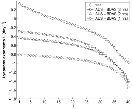
Figure 2: Effect of the observing system set-up on stability of the prediction-assimilation cycle for the Lorenz 40-variable model [32]. Spectrum of the Lyapunov exponents for the free system (1) (diamonds) and for the AUS-BDAS forced system (5), given different assimilation intervals $\tau=t_{k+1}-t_{k}$: 3 hr (squares), 2 hr (triangles) and 1 hr (circles).

Figure 2 shows the spectrum of the 40 Lyapunov exponents of the first model [32], using 200 years of simulation. The free system possesses 13 positive exponents ($\lambda^{+}$), of which the leading one ($\lambda_{max}$ = 0.336 day^-1) corresponds to a doubling time of 2.06 days; its Kaplan-Yorke dimension is approximately 27.05. At each assimilation time, the analysis is performed by AUS with a single BDAS mode ${\bf e}^{BDAS}_{k}$ in the specification of the gain matrix, Eq. (7). In this single-observation situation, the matrices ${\bf E}$ and ${\bf\Gamma}$ reduce to a column vector and to a scalar, respectively; the latter is estimated statistically using the innovations — which are scalars, in the present case — following the approach of [25].

A single observation, adaptively located where the current BDAS mode attains its maximum value, is sufficient to stabilize the system, so that $\lambda_{max}$ = $-0.283$ day^-1, and to reduce the RMS analysis error to 1.4$\%$ of the system’s natural variability, even when the assimilation interval $\tau=t_{k+1}-t_{k}$ is as long as 3 hr. Smaller assimilation intervals of 2 hr and 1 hr lead to further stabilize the system ($\lambda_{max}$ = $-0.437$ day^-1 and $-0.809$ day^-1, respectively), and thus to reduce the analysis error even more: the RMS error, normalized by the natural variability, becomes 0.011 and 0.009, respectively.

Figure 3 shows the first 100 Lyapunov exponents of the quasi-geostrophic model [34], using one year of simulated time. The free system possesses 24 positive exponents ($\lambda^{+}$), of which the leading one ($\lambda_{max}$ = 0.310 day^-1) corresponds to a doubling time of 2.2 days, and its Kaplan-Yorke dimension is approximately 65.2. The three assimilation experiments all use a fixed network of noisy observations that cover just under one-third of the domain (20 out of 64 meridional lines of grid points); in two of the experiments, an additional observation is adaptively located at a single grid point in the otherwise unobserved portion of the domain. Its location coincides with the maximum of a single BDAS mode, as in the first model [32]. The model time step is $\Delta t=30$ min, while the assimilation interval $\tau$ is 6 hr.

In all three experiments, the fixed observations are assimilated by a least-square fit, according to the three-dimensional variational (3DVar) algorithm [5, 9] in wide operational use, while the adaptive observations are assimilated either by 3DVar (3DVar-BDAS) or in the unstable subspace (AUS-BDAS) by using the current BDAS mode in Eq. (7). When fixed observations only are assimilated (3DVar), the number of positive exponents is reduced to three, with the leading exponent ($\lambda_{max}$ = 0.088 day^-1) corresponding to a doubling time of 7.9 days, while the Kaplan-Yorke dimension is reduced to 6.9 and the normalized RMS error to 0.321. Adding a single adaptive observation assimilated by 3DVar (3DVar-BDAS) stabilizes the prediction-assimilation cycle further, the only positive exponent being slightly greater than zero ($\lambda_{max}$ = 0.002 day^-1, Kaplan-Yorke dimension 1.1), and reduces the normalized RMS analysis error to around 0.16. Finally, when the adaptive observation is assimilated in the unstable subspace, the system is completely stabilized and the RMS analysis error drops to only 0.058.

4 Conclusion

To estimate the efficiency of prediction-assimilation systems and observational networks, one often estimates the error of a short-range forecast at points where fairly accurate observations are available; the obvious drawback of this approach is that errors tend to be smaller in systematically observed regions [3, 4, 26]. The nonlinear stability analysis introduced here allows one to address these issues in a more rigorous way. The stability of the prediction-assimilation system guarantees the uniqueness of its solution and is required for the convergence of this solution to the true flow evolution; in turn, the degree of stabilization introduced by the data assimilation may be measured precisely by estimating the full Lyapunov spectrum of the forced system.

Assimilation in the unstable subspace and the use of breeding on the prediction-assimilation system to estimate this subspace were applied here to a 40-variable [32] and to a 15 000-variable model [34] simulating the mid-latitude atmospheric circulation; in both models, the proposed methods led to complete stabilization of the sequential estimation process. The tools of dynamical systems theory can thus help design optimized assimilation algorithms (the specification of K) and observational networks (specifying ${\cal H}$) for high-dimensional and highly nonlinear systems. When, as usual in practical applications, only a limited number of measurements can be made, asymptotic error reduction may still be achieved through adaptive deployment of observations and a sophisticated assimilation scheme, designed to control the flow’s instabilities.

Data assimilation applications are possible in all situations where a dynamical constraint is important and only a limited amount of noisy observations can be taken. Such situations include robotics, flow in porous media, plasma physics, as well as solids subject to thermal and mechanical stresses or to shocks [35, 36]. The insights into the nonlinear dynamics of the prediction-assimilation cycle provided here should help design data assimilation methods for a large class of laboratory experiments [37], as well as for natural or industrial systems.

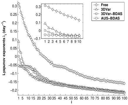
Figure 3: Effect of the assimilation method on stability for the quasi-geostrophic model [34]. Spectrum of the first 100 (the first 10 in the inset) Lyapunov exponents for the free system (1) (diamonds) and for the observationally forced systems (5): 3DVar (squares), 3DVar-BDAS (triangles) and AUS-BDAS (circles).

References

- [1] A. H. Jazwinki, Stochastic Processes and Filtering Theory, (Academic Press, 1970)
- [2] A. Gelb, Applied Optimal Estimation, (The MIT Press, 1974)
- [3] L. Bengtsson, M. Ghil and E. Källén, Dynamic Meteorology: Data Assimilation Methods, (Springer, 1981)
- [4] M. Ghil and P. Malanotte-Rizzoli, Adv. Geophys. 33, 141 (1991)
- [5] O. Talagrand, J. Met. Soc. Japan 75, 191 (1997)
- [6] R. Kalman, Trans. ASME, J. Basic Eng. 82, 35, (1960)
- [7] R. Kalman, Trans. ASME, Ser. D, J. Basic Eng. 83, 95 (1961)
- [8] M. Ghil, J. Met. Soc. Japan 75, 289 (1997)
- [9] E. Kalnay, Atmospheric Modeling, Data Assimilation and Predictability, (Cambridge University Press, 2003)
- [10] R. Todling and S.E. Cohn, Mon. Wea. Rev. 122, 2530 (1994)
- [11] M.K. Tippet, S.E. Cohn, R. Todling and D. Marchesin, J. Matrix Anal. Appl. 22, 56, (2000)
- [12] I. Fukumori, Mon. Wea. Rev. 130, 1370 (2002)
- [13] G. Evensen, J. Geophys. Res. 99, 143 (1994)
- [14] C.L. Keppenne and M.M. Rienecker, Mon. Wea. Rev. 130, 2951(2002)
- [15] S. E. Cohn and D. P. Dee, SIAM J. Numer. Anal. 25, 586 (1988)
- [16] E. Ott, C. Grebogi and J.A. Yorke, Phys. Rev. Lett. 64, 1196 (1990)
- [17] S. Boccaletti, C. Grebogi, Y.-C. Lai, H. Mancini and D. Maza, Physics Reports 329, 103 (2000)
- [18] M. Chen and J. Kurths, Phys. Rev. E 76, 027203, (2007)
- [19] E. Tziperman, H. Scher, S.E. Zebiak and M.A. Cane, Phys. Rev. Lett. 79, 1034 (1997)
- [20] G.S. Duane and J.J. Tribbia, Phys. Rev. Lett. 86, 4298, (2002)
- [21] G.S. Duane, J.J. Tribbia and J.B. Weiss, Nonlin. Processes Geophys. 13, 601 (2006)
- [22] S-C. Yang, D. Baker, H. Li, K. Cordes, M. Huff, G. Nagpal, E. Okereke, J. Villafane, E. Kalnay and G.S. Duane, J. Atmos. Sci. 63, 2340 (2006)
- [23] A. Trevisan and F. Uboldi, J. Atmos. Sci. 61, 103 (2004)
- [24] F. Uboldi and A. Trevisan, Nonlin. Processes Geophys. 13, 67 (2006)
- [25] A. Carrassi and A. Trevisan and F. Uboldi, Tellus 59A, 101 (2007)
- [26] M. Ghil, S. Cohn, J. Tavantzis, K. Bube and E. Isaacson, Applications of estimation theory to numerical weather prediction, in Dynamic Meteorology: Data Assimilation Methods, Springer, pp. 139–224 (1981)
- [27] K. Ide, P. Courtier, M. Ghil and A. Lorenc, J. Met. Soc. Japan 75, 181 (1997)
- [28] Z. Toth and E. Kalnay, Bull. Amer. Meteor. Soc. 74, 2317 (1993)
- [29] D.J. Patil, B.R. Hunt, E. Kalnay, J.A. Yorke and E. Ott, Phys. Rev. Lett. 86, 5878 (2001)
- [30] E.N. Lorenz, J. Atmos. Sci. 20, 130, (1963)
- [31] R.N. Miller, M. Ghil and F. Gauthiez , J. Atmos. Sci. 51, 1037 (1994)
- [32] E.N. Lorenz and K.A. Emanuel, J. Atmos. Sci. 55, 399 (1998)
- [33] D.K. Campbell, P. Rosenau and G. Zaslavsky (Eds.), 2005: The ”Fermi-Pasta-Ulam” Problem—The First 50 Years, Chaos, 15(1) (Special Issue).
- [34] R. Rotunno and J.W. Bao, Mon. Weather Rev. 124, 1051 (1996)
- [35] J. Kao, D. Flicker, R. Henninger, S. Frey, M. Ghil and K. Ide, J. Comput. Phys. 196, 705 (2004)
- [36] J. Kao, D. Flicker, K. Ide and M. Ghil, J. Comput. Phys. 214, 725 (2006)
- [37] M. J. Galmiche, Sommeria, E. Thivolle-Cazat and J. Verron, C. R. Acad. Sci. (Mécanique) 331, 843 (2003)