The Importance of Correlations and Fluctuations
on the Initial Source Eccentricity in High-Energy Nucleus–Nucleus Collisions
Abstract
In relativistic heavy-ion collisions, anisotropic collective flow is driven, event by event, by the initial eccentricity of the matter created in the nuclear overlap zone. Interpretation of the anisotropic flow data thus requires a detailed understanding of the effective initial source eccentricity of the event sample. In this paper, we investigate various ways of defining this effective eccentricity using the Monte Carlo Glauber (MCG) approach. In particular, we examine the participant eccentricity, which quantifies the eccentricity of the initial source shape by the major axes of the ellipse formed by the interaction points of the participating nucleons. We show that reasonable variation of the density parameters in the Glauber calculation, as well as variations in how matter production is modeled, do not significantly modify the already established behavior of the participant eccentricity as a function of collision centrality. Focusing on event-by-event fluctuations and correlations of the distributions of participating nucleons we demonstrate that, depending on the achieved event-plane resolution, fluctuations in the elliptic flow magnitude lead to most measurements being sensitive to the root-mean-square, rather than the mean of the distribution. Neglecting correlations among participants, we derive analytical expressions for the participant eccentricity cumulants as a function of the number of participating nucleons, , keeping non-negligible contributions up to . We find that the derived expressions yield the same results as obtained from mixed-event MCG calculations which remove the correlations stemming from the nuclear collision process. Most importantly, we conclude from the comparison with MCG calculations that the fourth order participant eccentricity cumulant does not approach the spatial anisotropy obtained assuming a smooth nuclear matter distribution. In particular, for the system, these quantities deviate from each other by almost a factor of two over a wide range in centrality. This deviation reflects the essential role of participant spatial correlations in the interaction of two nuclei.
pacs:
25.75.-q,25.75.Dw,25.75.GzI Introduction
One of the strongest pieces of evidence for the formation of a thermalized dense state of unconventional strongly interacting matter in ultra-relativistic nucleus-nucleus collisions at the Relativistic Heavy Ion Collider (RHIC) Arsene et al. (2005); Adcox et al. (2005); Back et al. (2005a); Adams et al. (2005a) stems from the strong anisotropic collective flow measured in non-central collision events Adcox et al. (2002); Adler et al. (2003, 2005); Back et al. (2002a, 2005b, 2005c); Ackermann et al. (2001); Adams et al. (2005b). Studies of the final charged particle momentum distributions have revealed strong collective effects in the form of anisotropies in the azimuthal distribution transverse to the direction of the colliding nuclei, and theory holds that their anisotropy around the beam axis in non-central collisions is established during the earliest stages of the evolution of the collision fireball Sorge (1997, 1999); Kolb et al. (2000); Heinz and Kolb (2002). The main component of this anisotropy is called “elliptic flow” and its strength is commonly quantified by the second coefficient, , in the Fourier decomposition of the azimuthal momentum distribution of observed particles relative to the reaction plane Poskanzer and Voloshin (1998).
By now there exists an extensive data set of elliptic flow measurements in collisions at RHIC as a function of center-of-mass energy, centrality, pseudo-rapidity and transverse momentum Adcox et al. (2002); Adler et al. (2003, 2005); Back et al. (2002a, 2005b, 2005c); Ackermann et al. (2001); Adams et al. (2005b). The magnitude of the observed flow anisotropy is found to be strongly correlated with the anisotropic shape of the initial nuclear overlap region. This is expected if interactions among the initially produced particles are very strong, leading to anisotropic pressure gradients, which transform the initial spatial eccentricity into a final momentum anisotropy Ollitrault (1992).
Quantitatively, the connection between initial spatial and final momentum anisotropy is explored by hydrodynamical calculations that, for a given equation of state, relate a given initial source distribution to the final momentum distribution of the produced particles. For collisions at the top RHIC energy, GeV, such calculations are in good agreement with the elliptic flow data at mid-rapidity Kolb et al. (2001a); Back et al. (2005a). From similar studies, it has been numerically established that, for not too large impact parameters, the final magnitude of the elliptic flow is proportional to the initial eccentricity, , used to characterize the spatial anisotropy in the transverse plane of the matter created in the overlap region of the colliding nuclei Kolb et al. (2000); Bhalerao et al. (2005). More generally, one expects the ratio of elliptic flow and eccentricity, , at mid-rapidity to be a universal function of density and size of the system at the time when the elliptic flow develops (“ scaling”) Heiselberg and Levy (1999); Voloshin and Poskanzer (2000); Bhalerao and Ollitrault (2006). In hydrodynamics, this function depends parametrically on the speed of sound in the fireball medium Bhalerao et al. (2005).
The elliptic flow in collisions at RHIC was found to be comparatively large, especially for near-central collisions, reaching almost the same magnitude as in collisions for the same fractional cross section Alver et al. (2007a); Adare et al. (2007), and much larger than expected from hydrodynamical models Hirano et al. (2005). A quantitatively meaningful comparison of the elliptic flow values measured in and collisions requires dividing out the difference in the eccentricity of the nuclear overlap zone since, for a given centrality, the average eccentricity depends on the size of the colliding nuclei. For the same size of the overlap zone similar densities are achieved in the two collision systems Alver et al. (2006); Roland et al. (2006), but the system exhibits a significantly smaller spatial eccentricity. If one scales the measured by this eccentricity, using its conventional definition in terms of the spatial deformation of the average transverse distribution of participating nucleons at a given impact parameter, one is led to the paradoxical finding that the smaller system translates the initial spatial deformation more efficiently into a final momentum anisotropy than the larger system Alver et al. (2006); Roland et al. (2006).
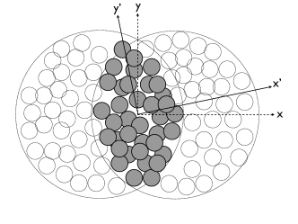
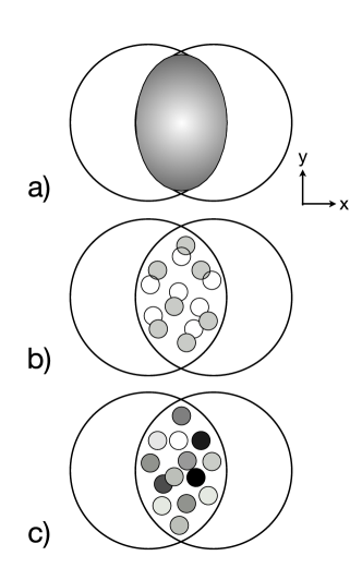
However, this conclusion depends on the definition of the eccentricity used in the scaling procedure. In LABEL:Miller:2003kd it was pointed out that the shape of the nuclear overlap fluctuates from event to event, and in LABEL:Manly:2005zy it is emphasized that the orientation of its major axes relative to the reaction plane (defined by the beam axis and impact parameter vector) fluctuates as well. This is illustrated in Fig. 1. For a given event, the actual distribution of the participant interaction points in the overlap zone can cause the overlap zone to be tilted with respect to the reaction plane. The participant eccentricity (, Eq. (14) Manly et al. (2006)) takes this into account by using the principal axes of the overlap zone. Because of the fluctuations, the ensemble average of the event-wise participant eccentricity is not identical with the standard eccentricity (, Eq. (10)) of the smooth overlap distribution which is obtained by averaging the participant density in the overlap region with respect to the reaction plane over many events.
Since hydrodynamic collective flow is not a property of the event ensemble, but rather develops independently in each collision event, its driving force is the shape and deformation of the initial distribution of produced matter in each event. To investigate the validity of the hydrodynamically predicted scaling one should therefore, in principle, compute the ratio event by event, before taking its ensemble average . This is, unfortunately, not possible in practise since the initial spatial eccentricity of a given collision event cannot be measured, and a statistically accurate determination of the elliptic flow also requires summing the hadron momentum spectra over many events, so only its ensemble average is known. In practise, the best way to approximate is to scale the measured elliptic flow by a calculated average participant eccentricity or by a higher moment of it (see below).
In LABEL:Manly:2005zy,Alver:2006wh the participant eccentricity scaling was studied using Monte Carlo Glauber (MCG) calculations, where is computed for each event from the transverse position distribution of nucleons participating in the collision, taken in its individual major axis frame. For large nuclei, event-wise fluctuations in the transverse density distributions are small, except for the most peripheral collisions. Nonetheless, as one approaches zero impact parameter (i.e. in almost central collisions where both and are tiny), these small density fluctuations still cause significant relative fluctuations of , resulting in a non-negligible difference between the participant and the standard eccentricity, even in collisions. For the smaller system the event-wise fluctuation effects are much stronger and seriously affect the eccentricity over the entire range of impact parameters Alver et al. (2007a). The participant-eccentricity-scaled elliptic flow thus differs appreciably from the standard eccentricity-scaled elliptic flow. It appears that scaling with the participant eccentricity unifies the eccentricity-scaled elliptic flow across the and collision systems Manly et al. (2006); Alver et al. (2007a), even differentially as a function of transverse momentum and pseudo-rapidity Alver et al. (2007b). Furthermore, first measurements of elliptic flow fluctuations have recently been reported in collisions at GeV Alver et al. (2007c); Sorensen (2007). The relative fluctuation magnitude from MCG is in striking agreement with from data Alver et al. (2007c), as expected if initial state fluctuations are combined with hydrodynamic evolution.
The initial success of the participant eccentricity calculated in the MCG approach immediately suggests a new set of questions:
-
•
How robust are the participant eccentricity results to the parameters characterizing the nuclear density distribution (radius, skin depth and nucleon–nucleon potential)?
-
•
What is the effect of varying the assumptions about matter production (locality, participant and binary collision weighting)?
-
•
What features of the MCG initial state distinguish it from the usual optical Glauber model picture?
-
•
More specifically, what is the impact of the fluctuating initial conditions on the suggested Miller and Snellings (2003); Bhalerao and Ollitrault (2006) use of cumulant approaches? In particular, which moment of an underlying fluctuating flow distribution is measured by the (standard) event-plane flow method Poskanzer and Voloshin (1998)?
These questions will be addressed in the present paper. In addition, following and improving on LABEL:Bhalerao:2006tp, we derive analytical expressions for the eccentricity cumulants in terms of moments of the initial spatial matter distribution, including all leading terms. Furthermore, by comparing with the numerical MCG model, we show that the analytical expressions are misleading as they neglect important effects arising from spatial correlations between the participating nucleons.
II Monte Carlo Glauber model
To estimate the geometrical configurations of colliding nuclei, one typically constructs models based on rather generic assumptions about the constituent makeup of a typical nucleus. In this context, it is fairly standard to assume that nuclear matter in a nucleus is distributed according to the charge distributions seen in electron scattering experiments. There are two ways of expressing these densities in actual calculations (for an overview, see LABEL:Miller:2007ri and references therein). One way is to assume a smooth matter density, typically described by a Fermi distribution in the radial direction and uniform over solid angle (in the case of spherical or near-spherical nuclei), as done in “optical” Glauber calculations Bialas et al. (1976, 1977). It should be noted that this method neglects some potentially important correlations between participating nucleon positions as will be discussed further in Section IV.3.
A related, but fundamentally different approach is to distribute, event-by-event in a stochastic manner, individual nucleons according to the smooth matter distribution and to evaluate the collision properties of the colliding nuclei by averaging over multiple events using Monte Carlo methods Ludlam et al. (1986); Shor and Longacre (1989). The key ingredients in MCG calculations are the following:
-
1.
The nucleon position centers in each nucleus are distributed according to a probability distribution given by the smooth nuclear density function, . One can think of the smooth nuclear density as a quantum mechanical single-particle probability distribution for the nucleon positions and their actual values in an individual collision event as a “measurement” of their positions in a given collision experiment.
-
2.
The nucleons are assumed to travel in straight trajectories along the beam direction throughout the reaction, i.e. their transverse positions are “frozen” during the short time when the two high-energy nuclei pass through each other.
-
3.
The nucleons interact with nucleons in the oncoming nucleus by means of the nucleon–nucleon inelastic cross section () appropriate for the beam energies under consideration (measured in proton-proton collisions). The nucleon–nucleon collisions occur and produce particles independently, i.e. dynamical correlations among the nucleon positions in the multi-particle nuclear wave function are assumed to be negligible. The only correlations in the model are of geometrical nature and due to clustering effects from the interaction process itself, as explained in Section IV.3.
Commonly, a nucleon–nucleon collision in the reaction is defined to occur if the Euclidean transverse distance between the centers of any two nucleons is less than the “ball diameter”,
| (1) |
More specifically, the steps of the PHOBOS Monte Carlo Back et al. (2005a) calculation for a single event are the following:
-
•
Impact parameter selection: The two nuclei are separated in the -direction by an impact parameter, , chosen randomly according to up to some large maximum (fm). Thus, nucleus is defined to be centered at in the transverse plane, while nucleus is centered at . In addition, both nuclei are centered at , since the longitudinal coordinate of each nucleus does not matter for the subsequent steps 111Throughout the paper, we will keep the common choice that the reaction plane, defined by the impact parameter and the beam direction, is given by the - and -axes, while the transverse plane is given by the - and -axes..
-
•
Makeup of nuclei: For each nucleus, we loop over the number of nucleons, and , and for each nucleon center point choose random, uniformly distributed azimuthal and polar angles, as well as a radius sampled randomly according to the radial density distribution . Additionally, to mimic excluded volume effects, one may require a minimum inter-nucleon separation distance () between the nucleon centers of all nucleons in the nucleus. This introduces a geometrical correlation among the nucleon positions. In the construction of the nuclei, we make sure that the center-of-mass of the nuclei is correctly positioned, i.e. we achieve , and by shifting all nucleon centers by the average offset determined after the positions of all nucleons in the nucleus have been generated. Thereby we ensure that the nuclear reaction and the otherwise arbitrary MC frames coincide.
-
•
Collision determination: For each nucleon in nucleus , we loop over the nucleons in nucleus . If the 2-dimensional Euclidean distance between the nucleon from and the nucleon from is less than as defined in Eq. (1), the number of collisions suffered by both nucleons is incremented by one. If no such nucleon–nucleon collision is registered for any pair of nucleons, then no nucleus–nucleus collision occurred. Counters for determination of the total (geometric) cross section are updated accordingly.
Having access to the number of collisions suffered by each nucleon according to this purely geometrical (classical) prescription allows straightforward calculation of , the number of nucleons which are struck at least once, and , the total number of nucleon–nucleon collisions. The latter is defined as the sum of collisions suffered by nucleons in one nucleus with nucleons from the other one (to avoid double counting). For every collision, the calculation keeps track of the position and status of each nucleon in the event, for later usage in the calculation of the spatial eccentricity or any other interesting quantity.
The default parameters of the PHOBOS Glauber calculations for and collisions at GeV are listed in Table 1. The nucleon–nucleon inelastic cross section of mb is from LABEL:Yao:2006px, while the parameters for the Fermi distribution,
i.e. the nuclear radius and the skin depth , are from LABEL:DeJager:1987qc. The minimum inter-nucleon separation distance is set to fm, i.e. we generally ignore geometrical correlations in the multi-nucleon wave function due to a hard core, since their effect, especially on the participant eccentricity, is found to be small, as we will report in Section III.1.
| System | [mb] | [fm] | [fm] | [fm] | |
|---|---|---|---|---|---|
| Parameter | Base | Min | Max | Base | Min | Max | |
|---|---|---|---|---|---|---|---|
| [mb] | |||||||
| [fm] | |||||||
| [fm] | |||||||
| [fm] | |||||||
A few comments are in order explaining what this model delivers and how we subsequently interpret its output. As described so far, the MCG model records only the (transverse) position and collision status of each nucleon. No particles are produced in the calculation and dynamical correlations among the nucleons in the nuclear wave function are neglected. By specifying the nuclear positions exactly, i.e. as long as we do not allow for a smearing around the points given by the model, we are prohibited (by quantum mechanical uncertainty) from imposing any constraints on the momenta of the scattered nucleons and, in consequence, of the particles produced by the collision. Source eccentricities calculated directly from the distribution of (exact) nucleon positions obtained from the MCG model can therefore, at least in principle, not immediately be assumed to represent the eccentricity of the produced matter distribution which drives the anisotropy of the subsequent collective expansion. For this reason, we extend in Section III.2 the model by smearing the resulting nucleon–nucleon collision points with a profile function in order to model the production of (approximately thermalized) matter with finite temperature and restricted particle momenta in the neighborhood of the collision points delivered by the MCG model. The (in-)sensitivity of the source eccentricity of these matter distributions to the parameters of the smearing profile is studied in detail.
III Robustness of the eccentricity
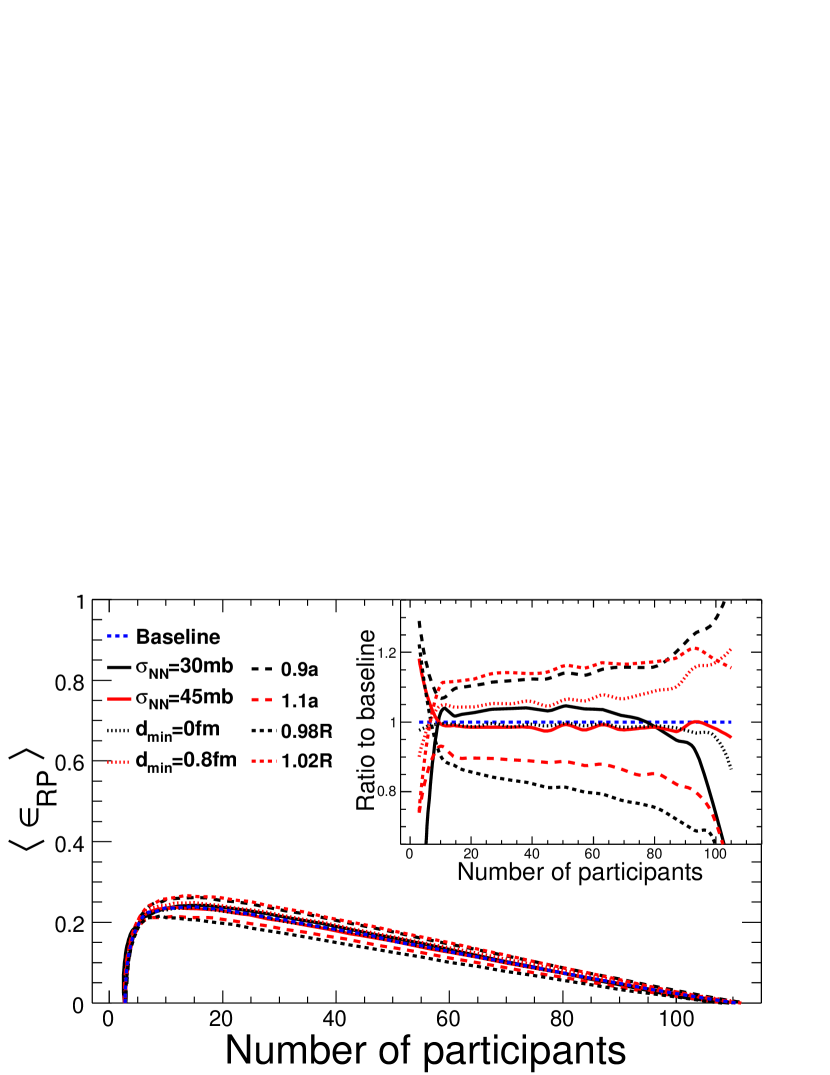
In this section, we evaluate the effects of variations in the nuclear density distributions and of various assumptions about the sources and spatial localization of the initial matter distributions on the eccentricity and its centrality dependence. The two definitions of eccentricity considered in this section are the reaction plane eccentricity (see Eq. (11))
and the participant eccentricity (see Eq. (14))
where , and are the (co-)variances of the participant-weighted nucleon distribution in a given MCG event 222Both definitions have already been used in Refs. Manly et al. (2006); Alver et al. (2007a).. Their definitions and relation to the standard eccentricity (, Eq. (10)) of the event-averaged distribution, are discussed in Appendix A.
III.1 Variation of Density Parameters
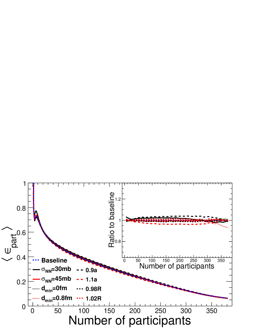
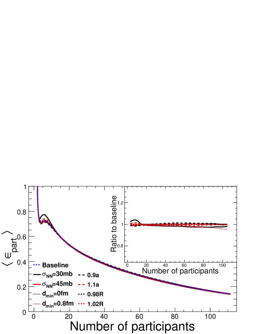
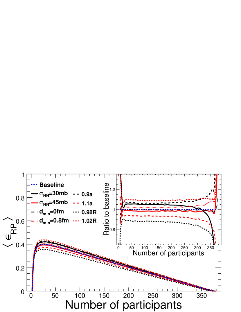
Before Refs. Miller and Snellings (2003); Manly et al. (2006) the purpose of MCG calculations was to estimate global properties of nucleus–nucleus collisions, i.e. to calculate centrality- and eccentricity-related quantities on average, based on (large) samples of Glauber events. Since both the participant eccentricity and the reaction plane eccentricity, explicitly involve an interpretation of each MCG event individually, it is important to understand their dependence on the choice of the MCG calculation parameters. A number of sources of systematic error are studied by varying a specific parameter with respect to the baseline parameter set as listed in Table 2. The baseline values for the sensitivity study correspond to the default parameter set for GeV except for the minimum inter-nucleon separation distance which is here set to fm to match the default value in HIJING Wang and Gyulassy (1991). We study the variation of all the main Glauber parameters except for the atomic mass number. The nuclear radius () is varied by %, the nuclear skin depth () by %; both variations are several times larger than the systematic error assigned to their measurements by the authors of LABEL:DeJager:1987qc. The nucleon–nucleon inelastic cross-section () is varied by more than the experimentally spanned region at RHIC 333A posteriori, this is justified since the dependence on turns out to be small. Thus, this approach will allow the treatment of the systematics at all collision energies in the same way.. The minimum inter-nucleon separation distance, which is not known experimentally, is varied by %. As one can see in Fig. 2, both eccentricity definitions are quite stable within the studied range of Glauber parameters. In particular, this is true for the participant eccentricity. Not unexpectedly, the difference between the two definitions, and , is most pronounced for . We have also found that varying two parameters at the same time does not increase significantly the observed variation in eccentricity.
III.2 Particle Production Models
III.2.1 Binary Collisions versus Participants
The observed particle multiplicity at mid-rapidity scales somewhat more strongly than linearly with the number of participating nucleons Back et al. (2004). This can be parametrized by postulating a second (smaller) contribution to particle production that scales with the number of binary nucleon–nucleon collisions Kharzeev and Nardi (2001). The MCG model as described above, can be extended to implement matter distributions produced according to a “two-component” scenario, where some of the matter is generated proportionally to the number of binary collisions. To add this feature, it is necessary to define two origins of matter production:
-
•
Participant nucleons, which create the matter by means of “exciting” the nucleon.
-
•
Binary nucleon–nucleon collisions, which create the matter locally via a two-body interaction.
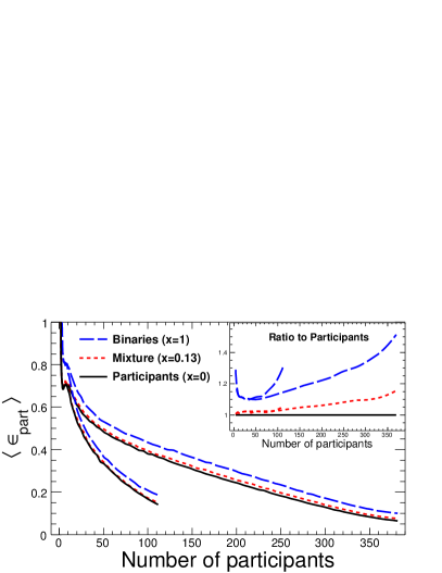
The latter mechanism suggests that the produced matter, to be incorporated into the calculation of spatial eccentricity, should be centered between the colliding nucleons. We achieve this by means of a “pseudo-particle” that is located at the center of mass of the pair of colliding nucleons and keeps track of the “collision-weighted” matter with an appropriate weight . Thus, contributions to the eccentricity from participants are weighted by while those from binary collisions by . In Fig. 3, the results for purely participant () and purely collision () weighted participant eccentricity are shown and compared to the case which has been found to describe the centrality dependence of the multiplicity at mid-rapidity according to Back et al. (2004). Independent of centrality, the collision weighted values are shifted to larger eccentricity for all centralities, similar to what is known for the standard eccentricity Kolb et al. (2001b). The presumably realistic case of yields about % larger eccentricity in the most central collisions.
III.2.2 Effects of Smeared Matter Distributions
The driving force for hydrodynamic elliptic flow is not directly the eccentricity of the distribution of participating nucleons or binary nucleon–nucleon collisions, but rather the anisotropy of the pressure gradients in the initially produced hot matter after it has thermalized. The transverse distribution of this matter will be smeared around the transverse positions of the participating nucleons or binary collision points. To study the behavior of the eccentricity under different definitions, we introduce a general procedure for incorporating a variety of matter density distributions. In this approach, the contribution of each matter production point (i.e. the center of a participant nucleon or a binary collision) at () is smeared according to , leading to a continuous weight function defined at all space-points in the transverse plane, . Averages and higher moments in space-time are then calculated (for individual events) using this weight function, e.g. . The point-like MCG cases described above correspond to the choice of . We look at two different, azimuthally symmetric, parametrizations for the smearing profile
-
•
Hard-sphere smearing,
-
•
Gaussian smearing,
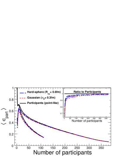
where and denotes the step function. In the following, we estimate meaningful choices for the parameters, and . For , it makes sense to use the interaction radius, , since the nucleons in the Glauber model are assumed to interact if their centers are within the “ball diameter” , Eq. (1). For GeV, this corresponds to fm. Then, matching the root-mean-square (RMS) width of the Gaussian distribution to the RMS width of the hard-sphere, , leads to fm. In Fig. 4 we show the results for the participant eccentricity calculated for point-like, hard-sphere, and Gaussian local matter distributions, using this set of parameters. The comparison reveals that for both collision systems the way the produced matter is distributed around the MCG interaction points does not significantly influence the observed value of the eccentricity except for extremely small systems. This also shows that the quantum mechanical uncertainty on the transverse positions of the interaction points has no major influence on the initial source eccentricity. Note that similarly to what was reported in LABEL:Broniowski:2007ft we find significantly different centrality dependence for if we allow smearing out the local matter sources to a very large extent. For example, in collisions at all centralities does not exceed for Gaussian smearing with fm.
IV Correlations and Fluctuations
In this section, we focus on eccentricity cumulants (which enter the discussion and interpretation of elliptic flow data) in the context of fluctuating initial conditions and for different realizations of the Glauber model initial state.
IV.1 Sensitivity of the Event-Plane Method
to Underlying Flow Fluctuations
There are different ways of extracting the elliptic flow from data: the event-plane method, two-particle correlations, multi-particle cumulants, etc. (see Refs. Poskanzer and Voloshin (1998); Borghini et al. (2001)). Each flow measurement is based on a different moment of the final-particle momentum distribution and thus is differently affected by event-by-event flow fluctuations (and non-flow correlations). If elliptic flow is proportional to the spatial anisotropy, the eccentricity scaling should be performed with corresponding moments of the participant eccentricity Miller and Snellings (2003); Bhalerao and Ollitrault (2006).
It has been explicitly stated Bhalerao and Ollitrault (2006) (see also Borghini et al. (2001)) that the event-plane method (), used by the PHOBOS experiment to measure elliptic flow, really measures rather than , i.e. the RMS rather than the mean of . More specifically, it has been claimed that depending on the event-plane resolution, with the upper limit being approximately reached under RHIC conditions Ollitrault (2006). Here, indicates an average over many collision events. In the following, we will investigate and confirm this claim.
In the event-plane method Poskanzer and Voloshin (1998), one uses the particles from one side of the detector (subevent ) to estimate the event plane, the plane relative to which the flow develops, given by . One then correlates the particles from the other, symmetric, side of the detector (subevent ) with this event plane to obtain the uncorrected flow signal for the given subevent, . Here, as before and in the appendices, indicates the average over an individual event. The roles of subevents and can then be interchanged to obtain , , and thus the observed flow signal for the whole event . Assuming small dynamical and non-flow correlations one has (for symmetric subevents)
| (2) |
where the average is, unlike before, not over particles in a given event but over events in the given centrality, and bin. In this equation, stands for the actual event plane angle, which defines the orientation of the signal in a particular event Alver et al. (2007a), and quantifies the event-plane resolution, which itself depends on Poskanzer and Voloshin (1998). The resolution can be estimated based on data alone,
| (3) |
leading to . The presence of a fraction () of uncorrelated background particles in addition to the particles that carry the flow signal corresponds (restricting ourselves to second harmonic contributions) to a distribution of
| (4) |
leading to an apparent suppression of the observed flow signal by . Correcting for this effect, we arrive at the final expression for the flow measured via the event-plane method
| (5) |
This includes the two main experimental corrections, namely for suppression and event-plane resolution Back et al. (2002a).
From Eq. (5) it is not obvious if the scales with the mean or the RMS of an underlying distribution, and how such a behavior depends on . However, one can study this behavior numerically with a MC calculation that creates events with distributed according to a given distribution, . For every event, we take particles (at mid-rapidity) to carry the flow signal, according to , and particles () to represent the uncorrelated background, which are added with a uniform azimuthal distribution. To relate the obtained to a moment of the input distribution, we implicitly define the exponent according to
| (6) |
where the ensemble average is calculated with the underlying distribution, . One obtains the sensitivity of the event-plane method to : corresponds to a scaling of with the mean, to a scaling with the RMS of , also often denoted Borghini et al. (2001). In our calculation, we choose to be uniformly distributed between and , i.e. the true mean and RMS are and , respectively.
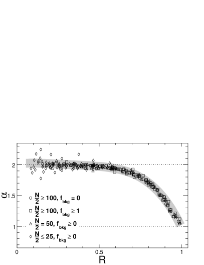
Fig. 5 shows the result of the calculation for various combinations of and between and , various values of between and , as well as values of between and . For each set of parameters, events have been simulated. The number of particles in each event is not allowed to fluctuate, i.e. exactly particles are created in every event. Within a reasonable spread that increases with decreasing resolution, the values are found to lie on a common curve as a function of , with no or weak dependence at most on the chosen simulation parameters. The PHOBOS measurements lie in the range of for and for where scales approximately with the RMS of the underlying distribution. This result is supported by recent, full detector simulations with HIJING MC events that incorporate known, but fluctuating, values. For the measured value of % Alver et al. (2007c) this implies that the PHOBOS measurements are about 10% larger than the mean elliptic flow.
IV.2 Participant-Eccentricity-Scaled Elliptic Flow
It is expected Heiselberg and Levy (1999); Voloshin and Poskanzer (2000) that scales with the transverse charged particle area density at mid-rapidity according to , where is the overlap area in the transverse plane. The data are measured in bins of centrality, translating into
| (7) |
Here, is the PHOBOS estimate of the ensemble-averaged elliptic flow according to Eq. (5), and is a suitable ensemble-averaged initial source eccentricity. In view of the discussion of the preceding subsection, is about , the RMS of the underlying distribution. Following the suggestion of Refs. Miller and Snellings (2003); Bhalerao and Ollitrault (2006) we therefore scale it with , the RMS of the participant eccentricity distribution obtained from the MCG model. The overlap area
corresponds to the area of the tilted overlap ellipse (see Appendix A, and especially Eq. (16)).
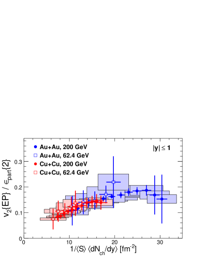
To arrive at the centrality average for and , we fold their dependence with the distribution of values obtained for each centrality bin from full detector simulations. Independent of species and energy, we scale the elliptic flow data by and the mid-rapidity yields by to convert from pseudo-rapidity () to rapidity () as described in LABEL:Adler:2002pu,Back:2004zg. Fig. 6 shows the result for and collisions at and GeV. The flow data are from Refs. Back et al. (2005b); Alver et al. (2007a), and the mid-rapidity yields from Refs. Back et al. (2002b, 2006); Alver et al. (2007d). We distinguish two types of errors that are individually propagated in the error calculation of the ratios: a) Systematic and statistical errors (if available) from data added in quadrature to obtain total % C.L., and b) systematic errors (% C.L.) assigned to the MC quantities obtained by the variation of Glauber parameters with respect to the individual baseline values (cp. Table 2). As reported earlier Manly et al. (2006); Alver et al. (2007a), we find a common scaling between the different systems. However, within the errors, it is difficult to tell whether the almost linear rise of the eccentricity-scaled elliptic flow breaks down at larger values of the area density which might indicate that the hydrodynamic limit is being reached at the top RHIC energy.
IV.3 Cumulants and Correlations
As mentioned above, it is suggested Miller and Snellings (2003) that higher order cumulant moments of should be proportional to analogously defined higher order cumulant moments of the eccentricity, including:
| (8) |
In LABEL:Bhalerao:2006tp Bhalerao and Ollitrault (B&O) attempted to derive expressions for and semi-analytically, making use of two strong approximations. First, the paper contains an implicit assumption that all of the participant positions are independent samples of some underlying distribution, or at least that any correlations between participants do not affect the eccentricity fluctuations Ollitrault (2006). Second, the expressions in LABEL:Bhalerao:2006tp were obtained using a Taylor expansion, leading to a power series in which is then truncated at . Based on these approximations, they concluded that is numerically equal to the standard eccentricity , vanishing for central () collisions. This would in turn imply that higher order cumulants of the flow such as are insensitive to fluctuations in the participant distribution. In this section we show that B&O’s assumptions are too strong and that for collisions differs significantly from when better approximations are made, especially when the role of correlations is taken into account, e.g. for the usual PHOBOS MCG calculations.
IV.3.1 Correlations of Nucleons in the Initial State
The first approximation in LABEL:Bhalerao:2006tp is to ignore the correlations between nucleon participant positions, even though we know that there are at least three sources for such correlations.
First, in order to contribute to the produced matter, the participating nucleons must hit each other, which causes a correlation. For instance, in the case of a peripheral collision with two or three participants, the overlap region of the nuclei may be something like fmfm but the nucleons will necessarily all be within about fm of each other or else they would not be participants. In general, the participant positions will tend to be more clustered in position space than a random distribution since each participating nucleon must hit another one.
Second, if there are two nucleons from a given nucleus which are close together in transverse position, then they will have a tendency to be both hit or neither hit. Again this will contribute to clustering of participant positions.
The usual, full PHOBOS MCG calculation takes both of these effects into account automatically, but the analytical expressions, given in LABEL:Bhalerao:2006tp and in Appendix B here, do not. The two different approximations are illustrated in Fig. 7 (panels a) and b)).
It should be noted that a precise integral Glauber calculation at fixed impact parameter should involve a complete -dimensional integral covering all possible transverse positions of all nucleons involved in the collision Czyz and Maximon (1969); Białas and Czyz (2001); Miller et al. (2007). Such a formulation would include the same correlations that are covered automatically by a MCG. The usual practise of approximating the Glauber integral with a single 2-dimensional integral (optical Glauber model approximation) is just an approximation which neglects all the correlations described above.
A third type of correlation would be genuine nucleon–nucleon position correlations in the wave functions of the nuclei that, as mentioned before, generally are ignored in all Glauber model calculations.
IV.3.2 Uncorrelated Glauber Monte Carlo
In order to estimate the role of pairwise spatial correlations among the participant nucleons in a nucleus–nucleus collision, we make use of a modified version of the MCG code. In the modified version, at first a normal event is calculated of which we record the impact parameter and corresponding number of participants. Then, a mixed event is constructed from independently calculated events, which are all required to have the same global characteristics, i.e. the same impact parameter and number of participants. From each such event, we choose one of the participating nucleons, such that in the constructed mixed event none of the participating nucleons is correlated to any of the other participants. The resulting approximation of the overlap density is illustrated in panel c) of Fig. 7.
Fig. 8 shows the comparison of the full PHOBOS MCG calculation with the mixed-event MCG calculation for the participant eccentricity and its first two cumulants. We find that the contribution of correlations to , and is quite important for the smaller system, i.e. it is about –% for and about –% for and rather constant over a wide range of centrality. Note that the structure seen in Fig. 8 at very low values (see also Figs. 2,3 and 4) is genuine for the full MCG and not present in the mixed-event case. Furthermore, spatial correlations among the participants in the initial state modeled by MCG are found to be less important for the reaction plane and standard eccentricity definitions (not shown). For both definitions the uncorrelated cases lead to slightly larger eccentricities. The deviation between full and mixed-event MCG decreases with increasing centrality and is less than a few percent for the and about –% for the system.
IV.3.3 Cumulants in the Extended B&O Approach
The second approximation in LABEL:Bhalerao:2006tp is to derive expressions for and using a Taylor expansion that leads to a power series in . In Appendix B, we advance the calculations to higher orders in by generalizing Eq. (11) from LABEL:Bhalerao:2006tp, and show how to obtain the analytical terms in a rigorous fashion. For , we obtain the same expression as Eq. (12) in LABEL:Bhalerao:2006tp, and prove that the terms are really negligible. We also obtain the expansion for , Eq. (53), where —in contrast to LABEL:Bhalerao:2006tp— all important terms have been kept. In particular, for central collisions, when , some terms of are not negligible and must be kept.
The values for the ensemble averages over participant nucleon distributions (like for example or ) in Eq. (53) need to be calculated numerically. We calculate each of these averages as a function of using the usual (full) PHOBOS MCG code. Inserting the numerically evaluated values into Eq. (53), leads to the “semi-analytic” result discussed below.
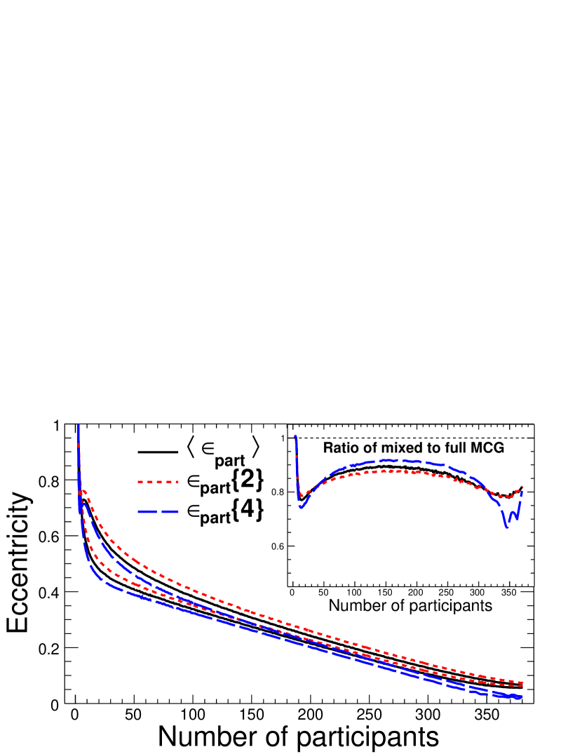
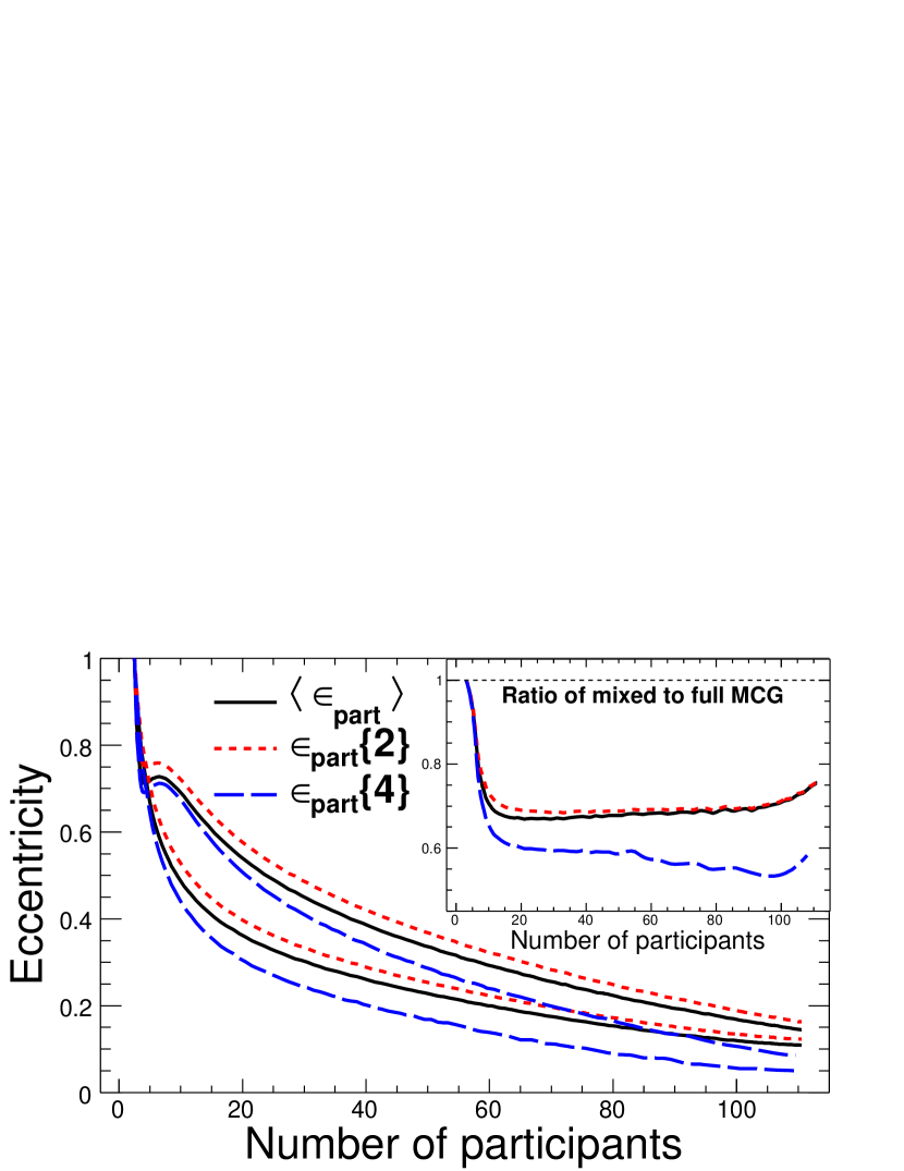
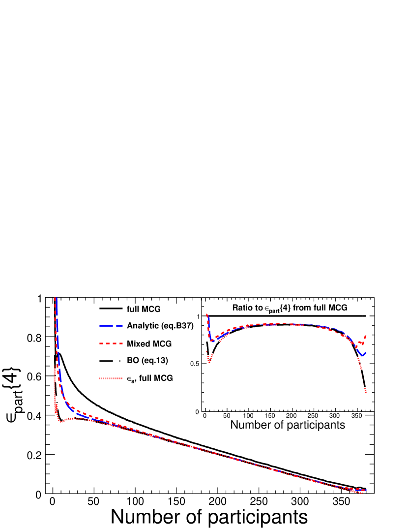
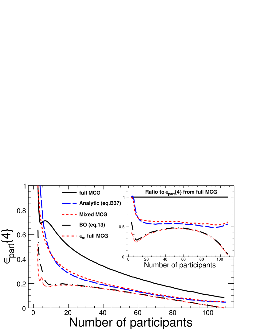
Fig. 9 shows the results for , comparing the full PHOBOS and mixed-event MCG with our semi-analytical result Eq. (53), and with B&O’s semi-analytical approximation (Eq. (13) from LABEL:Bhalerao:2006tp evaluated with the full PHOBOS MCG), as well as with the standard eccentricity . For both collision systems, our semi-analytical result fully agrees with the mixed-event MCG calculation. This is consistent with the fact that correlations among the participants are neglected in the analytical derivation of Eq. (53). Furthermore, it confirms that all numerically important terms have been kept in Eq. (53). The full MCG calculation which includes participant spatial correlations disagrees with the other calculations that neglect them by almost a factor of two. Contrary to LABEL:Bhalerao:2006tp, we find that, for the system, calculated in the semi-analytical approach does not agree with , in particular for very peripheral and near-central collisions. More important, however, is the aforementioned effect of the neglected correlations. For the system, is found to be numerically close to (with deviations of less than %) over a wide range of centralities. Only for very peripheral and near-central collisions correlations may play an important role. For the system, on the other hand, differs from by almost a factor of two over a wide range of centralities, implying that correlations can not be neglected for the smaller system.
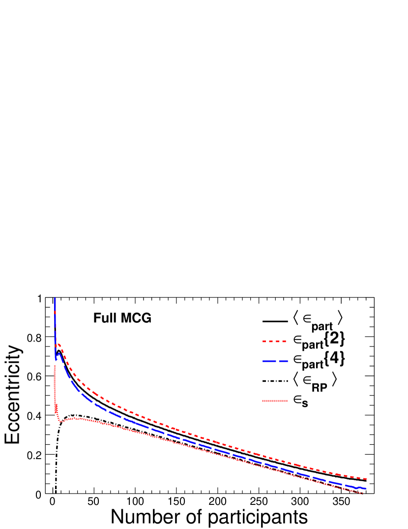
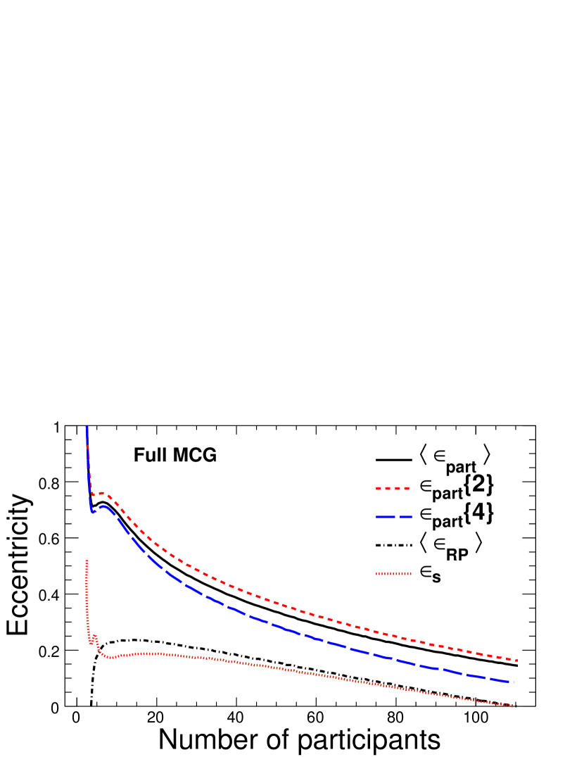
Fig. 10 shows a comparison of all eccentricity definitions used in the present paper (participant eccentricity and cumulants, reaction plane and standard eccentricity), obtained from full MCG calculations with baseline parameters listed in Table 1.
As mentioned before, in contrast to the results shown in Fig. 9, the authors of LABEL:Bhalerao:2005mm find in their work that differs very little from both the standard eccentricity and the average reaction plane eccentricity , the latter two being almost equal. Recently, the authors of LABEL:Voloshin:2007pc have shown that, within a Gaussian model of the event-by-event eccentricity fluctuations, the identity of with is exact (see Eq. (9) in Voloshin et al. (2007)) as long as the Gaussian widths for and for the correlation term are equal. We were able to trace the inequality between and present in our MCG model (see Fig. 10) to a breakdown of the Gaussian model assumptions made in LABEL:Voloshin:2007pc, in particular for peripheral collisions and small collision systems. We find that in the MCG model the event-by-event fluctuations of the correlation term are indeed Gaussian for mid-central to central and most central collisions. On the other hand, the event-by-event fluctuations of are not well described by a Gaussian function for all and collisions except the most central ones. Furthermore, for semiperipheral and peripheral collisions the width of the distribution does not agree with the width of . Consequently, for all but the most central collisions, our MCG model results are poorly described by the Bessel-Gaussian distribution given in Eq. (3) of LABEL:Voloshin:2007pc on which the equality of and is based.
V Conclusions
The interpretation of the anisotropic flow data measured in nucleus–nucleus collisions at high energy requires a detailed understanding of the initial source anisotropy, which is typically quantified by the eccentricity of the shape of the nuclear overlap area. In this paper, we investigate various ways of defining this effective eccentricity using MCG calculations.
We find that variations in the Glauber parameters have only small effects on the participant eccentricity for both the and collision systems, while the reaction plane eccentricity shows variations on the % level (Fig. 2). The generalization from participant-weighted to collision-weighted interaction point distributions leads to an increase in the obtained participant eccentricity, by a constant shift, similarly to what is known for the standard eccentricity (Fig. 3). Over a realistic range of parameters, the modeling of smeared matter distributions does not lead to significantly different results for the participant eccentricity (Fig. 4). Thus, we conclude that reasonable variations in density parameters, the sources of matter, and their localization have only a small effect on the participant eccentricity. These results support our initial idea Manly et al. (2006); Alver et al. (2007a) to use the participant eccentricity definition in conjunction with elliptic flow scaling.
Depending on the event-plane resolution, fluctuations in the elliptic flow magnitude influence the measured “mean” , and for low resolution bias the measurement towards the RMS of the elliptic flow distribution. For a given event-plane resolution, we find that there is a simple connection with the appropriate moment of , which appears to be independent of the level of uncorrelated background (Fig. 5). For the resolutions achieved with the PHOBOS elliptic flow method Back et al. (2002a) this gives a scaling with the RMS of for all measured systems and energies. We take this into account in the eccentricity-scaled elliptic flow (Fig. 6) by presenting it as together with individual systematic errors from data and MC parameter variations. The participant-eccentricity-scaled elliptic flow shows an almost linear scaling with the particle area density as predicted in Refs. Heiselberg and Levy (1999); Voloshin and Poskanzer (2000) in the low density limit.
A rigorous attempt to analytically derive non-negligible contributions to cumulants of the participant eccentricity distribution out to confirms the expressions found in LABEL:Bhalerao:2006tp, for all but , where our derivation, Eq. (53), for the first time keeps all leading order terms in the series. The numerical evaluation of our analytical result for agrees with obtained with the mixed-event MCG calculation, as expected, since both ignore all correlations among the participating nucleons. In comparison, the results obtained from full PHOBOS MCG calculations, which include spatial correlations among the participants, imply that pairwise spatial correlations among the participants from the collision process itself are quite important, especially for the system. For the contribution to the participant eccentricity cumulants is about –%, while it is about % over most of the centrality range for (Fig. 8). Furthermore, it turns out that for the system differs from by about a factor of two, while the difference for is smaller and only about % for most of the centrality range (Fig. 9, Fig. 10). Therefore, while correlations among participating nucleons may be neglected at the % accuracy level over a wide range of centralities in the larger system, they are crucially important for the smaller system and should not be neglected. These results suggest that correlations among participants that are certainly present in nature and that are to a large extent implemented in full MCG calculations are sufficiently important that they should be taken into account in any study where nuclear geometry is expected to play an important role.
Acknowledgements.
Fruitful discussions with Arthur K. Kerman, John W. Negele and Jean-Yves Ollitrault are acknowledged. This work was partially supported by U.S. DOE grants DE-AC02-98CH10886, DE-FG02-93ER40802, DE-FG02-94ER40818, DE-FG02-94ER40865, DE-FG02-99ER41099, and DE-AC02-06CH11357, by U.S. NSF grants 9603486, 0072204, and 0245011, by Polish KBN grant 1-P03B-062-27(2004-2007), by NSC of Taiwan Contract NSC 89-2112-M-008-024, and by Hungarian OTKA grant (F 049823). The work of U.H. was supported by the U.S. DOE under grant DE-FG02-01ER41190.Appendix A Eccentricity Definitions
The spatial anisotropy of the interaction region in the transverse plane (in the following as throughout the paper given by the - and -axes) is commonly called “eccentricity” and denoted with the symbol . It has been introduced in LABEL:Heiselberg:1998es (called “deformation”, symbol ) and in LABEL:Sorge:1998mk (called “spatial asymmetry”, symbol ), while the basic idea of a dimensionless momentum-based anisotropy parameter (symbol ) originates from LABEL:Ollitrault:1992bk. In its most basic formulation, the eccentricity definition reads
| (9) |
where and characterize the size of the source in the - and -direction, respectively. Note that this definition allows positive and negative values, . It is related, but not identical, to the geometrical definition of the eccentricity of an ellipse. In this appendix, we will summarize the most important definitions of eccentricity.
A.1 Standard Eccentricity
Prior to our work Manly et al. (2006), it has been common practise to use smooth, event-averaged initial conditions, for which the initial spatial asymmetry in the transverse plane has typically been given by the “standard” eccentricity
| (10) |
where and are the second moments of the (typically participant-weighted) ensemble-averaged nucleon distribution in the - and -direction, respectively. We follow the notation introduced by Bhalerao & Ollitrault in LABEL:Bhalerao:2006tp, where denotes an average taken over many events (ensemble average), while stands for an average (over participants) in a single event (sample average).
A.2 Reaction Plane Eccentricity
The two incoming nuclei, separated by the impact parameter , can be assumed to be centered at (,0) in the transverse plane such that for a given event the chosen MC frame coincides with the nuclear reaction frame. The “reaction plane” eccentricity is then obtained from
| (11) |
where and are the (typically participant-weighted) variances of the nucleon distribution in - and -direction in a given event. In contrast to , which is only defined for the entire ensemble of collision events, is defined for each event and has its own ensemble average . The reaction plane eccentricity can be useful in comparisons with data where the reaction plane is determined by spectator neutrons in a zero-degree calorimeter Bhalerao and Ollitrault (2006). Since is numerically very similar to (in the difference for is at most %, however in the difference is generally between –%, see also Fig. 10), it has been used in connection with MCG calculations in place of the standard eccentricity 444In Refs. Manly et al. (2006); Alver et al. (2007a) the reaction plane eccentricity was instead named or ..
A.3 Participant Eccentricity
The “participant” eccentricity expresses the overlap eccentricity in the rotated (“participant”) frame (see Fig. 1), denoted by and , which for a given event maximizes and minimizes . In principle, the overlap zone will also be shifted with respect to the reaction plane frame, but this shift has no impact on the eccentricity. Generally, the second moments of the position distribution in the nuclear reaction plane (or MC) frame are described by the covariance matrix,
| (12) |
where , and are the per-event (co-)variances of the underlying (typically participant weighted) nucleon distribution in the transverse plane, given in the original frame. The participant frame corresponds to the frame in which is diagonal. Since is a real symmetric matrix, its diagonalization can be accomplished by finding the eigenvalues that satisfy , leading to a second order polynomial in with two solutions:
| (13) |
These two values of correspond to and with the larger value () corresponding to the and the smaller value () to the direction, by definition. This leads to the expression for the participant eccentricity Manly et al. (2006); Alver et al. (2007a),
| (14) |
Like , the participant eccentricity is defined on an event-wise basis, however in contrast to the previous definitions of the eccentricity, it is non-negative, covering the range by construction. The participant frame is tilted event-by-event by an angle of with respect to the reaction plane, where
| (15) |
It should also be noted that since the overlap ellipse is generally tilted, its area is not proportional to as often assumed, but rather given by
| (16) |
Numerically the ratio, , is very similar for the and systems at the same , larger than 0.75, and increasing with increasing centrality so that for it is larger than 0.9 in GeV collisions.
Appendix B Calculating Cumulants
In LABEL:Bhalerao:2006tp Bhalerao & Ollitrault (B&O) derive the behavior of various cumulant moments of the participant eccentricity analytically, making use of two questionable approximations. First, the paper contains an implicit assumption that all of the participant positions are independent samples of some underlying distribution, or at least that any correlations between participants are unimportant to the eccentricity fluctuations Ollitrault (2006). Second, the paper uses a Taylor expansion which leads to a power series in which is then truncated at without proof that the nominally higher order terms are actually smaller.
In this appendix, we will extend the B&O results for the case in which any correlations between participant positions are still considered negligible, but keeping all important terms of the Taylor expansion. In particular, we will generalize Eqs. (11)–(14) of LABEL:Bhalerao:2006tp and comment on Eq. (8).
B.1 Generalizing B&O Equation 11
Following B&O, we will assume that for each event participants are generated independently from an arbitrary underlying 2-dimensional distribution. The averaging symbol denotes the average of the quantity over the underlying distribution and/or the ensemble average value taken over a large number of events. In order to investigate fluctuations, we must also consider event-wise averages . The event-by-event fluctuations are given by . For convenience of calculation, let us also define such that .
Obviously,
| (17) |
Next, we evaluate by exhibiting the ensemble and event averages explicitly:
| (18) |
The sums are all finite and their order can be interchanged freely. If the participants are numbered randomly, then . For example, the average of the values for all “participants number 7” over all events will just be . Correspondingly, . For we have
| (19) |
For with we have
| (20) |
since, following B&O, the positions of participants and () in each event are assumed to be uncorrelated. It is this last step in Eq. (20) which fails when there are correlations between the locations of different participants. Neglecting such correlations, as in B&O, one finally arrives at
| (21) | |||||
in agreement with Eq. (11) from B&O Bhalerao and Ollitrault (2006).
Generalizing the above derivation to higher orders, we, as well as Ollitrault Ollitrault (2006), find that the correct generalization of Eq. (21) for terms is given by
| (22) |
Compared to the terms, Eq. (21), this is suppressed by a factor . Starting with the term, the expressions begin to get more complicated. In particular,
| (23) | |||||
which is actually , i.e. the same order in the number of participants as the term.
The fifth and sixth order terms can be calculated similarly. Any terms involving single powers like will again vanish. The nonzero terms are
and
| (25) | |||||
In general, the dominant terms in the expansion should be those composed of products of bilinears like in the case of even powers of , and those with bilinears and one trilinear in the case of odd powers of . So, we have for and for . This means that we must consider terms up to if we want to find all terms in the series truncated by B&O, and terms up to in order to capture the leading behavior in the limit (see below).
B.2 B&O Equation 8
The Taylor expansion which leads to Eq. (8) in B&O is not applicable everywhere as it implicitly assumes that . Since for central collisions, this quantity is not guaranteed to be small, and this expansion is poorly behaved and formally divergent for central collisions. Fortunately, Eq. (8) of B&O is not actually needed in order to derive and generalize their Eqs. (12)–(14).
B.3 B&O Equation 12: Calculating
In order to calculate , we must first express in terms of the ’s. We start with the definition, Eq. (14):
| (26) |
Following B&O we have
| (27) | |||||
| (28) | |||||
| (29) |
using . This leads to the exact result:
| (30) | |||||
where . The second and third terms in the denominator are genuinely , so it can be safely Taylor expanded. The resulting polynomial series is well behaved. The leading terms are and . All terms of and higher are and can be dropped since they are at least a full power of down without any compensating factors. So, we obtain
| (31) | |||||
This leads to the same result as B&O Eq. (12), except that we have also shown that all further terms are subdominant:
| (32) | |||||
Similarly, Eq. (14) in B&O is well-behaved and correctly contains all of the leading terms. As noted above, this is different for the expansion of Eq. (8) in B&O, which does not converge in the limit .
B.4 B&O Equation 13: Calculating
We know from B&O that the terms cancel, leaving the term as apparently dominant. However, in order to confirm this, we need to check that all of the nominally higher order terms are actually small.
In order to organize the calculation, let us write the expansion of Equation (30) as:
| (33) |
where contains all terms of , of , and so on. Furthermore, let us define and etc., so that
| (34) |
Explicitly, we will need the following equations:
| (35) | |||||
| (36) | |||||
| (38) | |||||
| (39) | |||||
| (40) | |||||
We can now calculate :
| (41) | |||||
where we have kept all terms up to , and the leading terms in at and . We evaluate the expressions in Eq. (41) piece by piece, dropping any terms that would contribute to at or for each . Note that . This leads to the following expressions:
| (43) | |||||
| (44) | |||||
| (45) | |||||
| (46) | |||||
| (47) | |||||
| (50) | |||||
| (51) | |||||
| (52) |
Assembling, this leads to the final result
| (53) | |||||
where we now have all of the leading terms. Terms which have been dropped are down from the leading terms by at least a full factor of without any compensating factor. B&O Bhalerao and Ollitrault (2006) left out the term and most importantly the term. For , the term tends to be comparable to the “leading” term. For central collisions, as vanishes, the term becomes dominant and certainly cannot be neglected.
References
- Arsene et al. (2005) I. Arsene et al. (BRAHMS), Nucl. Phys. A757, 1 (2005), eprint arXiv:nucl-ex/0410020.
- Adcox et al. (2005) K. Adcox et al. (PHENIX), Nucl. Phys. A757, 184 (2005), eprint arXiv:nucl-ex/0410003.
- Back et al. (2005a) B. B. Back et al. (PHOBOS), Nucl. Phys. A757, 28 (2005a), eprint arXiv:nucl-ex/0410022.
- Adams et al. (2005a) J. Adams et al. (STAR), Nucl. Phys. A757, 102 (2005a), eprint arXiv:nucl-ex/0501009.
- Adcox et al. (2002) K. Adcox et al. (PHENIX), Phys. Rev. Lett. 89, 212301 (2002), eprint arXiv:nucl-ex/0204005.
- Adler et al. (2003) S. S. Adler et al. (PHENIX), Phys. Rev. Lett. 91, 182301 (2003), eprint arXiv:nucl-ex/0305013.
- Adler et al. (2005) S. S. Adler et al. (PHENIX), Phys. Rev. Lett. 94, 232302 (2005), eprint arXiv:nucl-ex/0411040.
- Back et al. (2002a) B. B. Back et al. (PHOBOS), Phys. Rev. Lett. 89, 222301 (2002a), eprint arXiv:nucl-ex/0205021.
- Back et al. (2005b) B. B. Back et al. (PHOBOS), Phys. Rev. C72, 051901 (2005b), eprint arXiv:nucl-ex/0407012.
- Back et al. (2005c) B. B. Back et al. (PHOBOS), Phys. Rev. Lett. 94, 122303 (2005c), eprint arXiv:nucl-ex/0406021.
- Ackermann et al. (2001) K. H. Ackermann et al. (STAR), Phys. Rev. Lett. 86, 402 (2001), eprint arXiv:nucl-ex/0009011.
- Adams et al. (2005b) J. Adams et al. (STAR), Phys. Rev. C72, 014904 (2005b), eprint arXiv:nucl-ex/0409033.
- Sorge (1997) H. Sorge, Phys. Rev. Lett. 78, 2309 (1997), eprint arXiv:nucl-th/9610026.
- Sorge (1999) H. Sorge, Phys. Rev. Lett. 82, 2048 (1999), eprint arXiv:nucl-th/9812057.
- Kolb et al. (2000) P. F. Kolb, J. Sollfrank, and U. Heinz, Phys. Rev. C62, 054909 (2000), eprint arXiv:hep-ph/0006129.
- Heinz and Kolb (2002) U. Heinz and P. F. Kolb, Nucl. Phys. A702, 269 (2002), eprint arXiv:hep-ph/0111075.
- Poskanzer and Voloshin (1998) A. M. Poskanzer and S. A. Voloshin, Phys. Rev. C58, 1671 (1998), eprint arXiv:nucl-ex/9805001.
- Ollitrault (1992) J.-Y. Ollitrault, Phys. Rev. D46, 229 (1992).
- Kolb et al. (2001a) P. F. Kolb, P. Huovinen, U. Heinz, and H. Heiselberg, Phys. Lett. B500, 232 (2001a), eprint arXiv:hep-ph/0012137.
- Bhalerao et al. (2005) R. S. Bhalerao, J.-P. Blaizot, N. Borghini, and J.-Y. Ollitrault, Phys. Lett. B627, 49 (2005), eprint arXiv:nucl-th/0508009.
- Heiselberg and Levy (1999) H. Heiselberg and A.-M. Levy, Phys. Rev. C59, 2716 (1999), eprint arXiv:nucl-th/9812034.
- Voloshin and Poskanzer (2000) S. A. Voloshin and A. M. Poskanzer, Phys. Lett. B474, 27 (2000), eprint arXiv:nucl-th/9906075.
- Bhalerao and Ollitrault (2006) R. S. Bhalerao and J.-Y. Ollitrault, Phys. Lett. B641, 260 (2006), eprint arXiv:nucl-th/0607009.
- Alver et al. (2007a) B. Alver et al. (PHOBOS), Phys. Rev. Lett. 98, 242302 (2007a), eprint arXiv:nucl-ex/0610037.
- Adare et al. (2007) A. Adare et al. (PHENIX), Phys. Rev. Lett. 98, 162301 (2007), eprint arXiv:nucl-ex/0608033.
- Hirano et al. (2005) T. Hirano, M. Isse, Y. Nara, A. Ohnishi, and K. Yoshino, Phys. Rev. C72, 041901 (2005), eprint arXiv:nucl-th/0506058.
- Alver et al. (2006) B. Alver et al. (PHOBOS), Phys. Rev. Lett. 96, 212301 (2006), eprint arXiv:nucl-ex/0512016.
- Roland et al. (2006) G. Roland et al. (PHOBOS), Nucl. Phys. A774, 113 (2006), eprint arXiv:nucl-ex/0510042.
- Miller and Snellings (2003) M. Miller and R. Snellings (2003), eprint arXiv:nucl-ex/0312008.
- Manly et al. (2006) S. Manly et al. (PHOBOS), Nucl. Phys. A774, 523 (2006), eprint arXiv:nucl-ex/0510031.
- Alver et al. (2007b) B. Alver et al. (PHOBOS), J. Phys. G34, S887 (2007b), eprint nucl-ex/0701054.
- Alver et al. (2007c) B. Alver et al. (PHOBOS), submitted to Phys. Rev. Lett. (2007c), eprint arXiv:nucl-ex/0702036.
- Sorensen (2007) P. Sorensen (STAR), J. Phys. G34, S897 (2007), eprint nucl-ex/0612021.
- Miller et al. (2007) M. L. Miller, K. Reygers, S. J. Sanders, and P. Steinberg (2007), eprint arXiv:nucl-ex/0701025.
- Bialas et al. (1976) A. Bialas, M. Bleszynski, and W. Czyz, Nucl. Phys. B111, 461 (1976).
- Bialas et al. (1977) A. Bialas, M. Bleszynski, and W. Czyz, Acta Phys. Polon. B8, 389 (1977).
- Ludlam et al. (1986) T. W. Ludlam, A. Pfoh, and A. Shor (1986), Brookhaven National Laboratory Report - BNL-37196 (Feb. 1986).
- Shor and Longacre (1989) A. Shor and R. S. Longacre, Phys. Lett. B218, 100 (1989).
- Yao et al. (2006) W. M. Yao et al. (Particle Data Group), J. Phys. G33, 1 (2006).
- De Jager et al. (1987) C. W. De Jager, H. De Vries, and C. De Vries, Atom. Data Nucl. Data Tabl. 36, 495 (1987).
- Wang and Gyulassy (1991) X.-N. Wang and M. Gyulassy, Phys. Rev. D44, 3501 (1991).
- Back et al. (2004) B. B. Back et al. (PHOBOS), Phys. Rev. C70, 021902 (2004), eprint arXiv:nucl-ex/0405027.
- Kharzeev and Nardi (2001) D. Kharzeev and M. Nardi, Phys. Lett. B507, 121 (2001), eprint arXiv:nucl-th/0012025.
- Kolb et al. (2001b) P. F. Kolb, U. W. Heinz, P. Huovinen, K. J. Eskola, and K. Tuominen, Nucl. Phys. A696, 197 (2001b), eprint hep-ph/0103234.
- Broniowski et al. (2007) W. Broniowski, P. Bozek, and M. Rybczynski (2007), eprint arXiv:0706.4266.
- Borghini et al. (2001) N. Borghini, P. M. Dinh, and J.-Y. Ollitrault, Phys. Rev. C64, 054901 (2001), eprint arXiv:nucl-th/0105040.
- Ollitrault (2006) J.-Y. Ollitrault, private communication (2006).
- Adler et al. (2002) C. Adler et al. (STAR), Phys. Rev. C66, 034904 (2002), eprint arXiv:nucl-ex/0206001.
- Back et al. (2002b) B. B. Back et al. (PHOBOS), Phys. Rev. C65, 061901 (2002b), eprint arXiv:nucl-ex/0201005.
- Back et al. (2006) B. B. Back et al. (PHOBOS), Phys. Rev. C74, 021901 (2006), eprint arXiv:nucl-ex/0509034.
- Alver et al. (2007d) B. Alver et al. (PHOBOS), submitted to Phys. Rev. Lett. (2007d), eprint arXiv:0709.4008 [nucl-ex].
- Czyz and Maximon (1969) W. Czyz and L. C. Maximon, Annals Phys. 52, 59 (1969).
- Białas and Czyz (2001) A. Białas and W. Czyz, private communication (2001).
- Voloshin et al. (2007) S. A. Voloshin, A. M. Poskanzer, A. Tang, and G. Wang (2007), eprint arXiv:0708.0800.