Dynamical analysis on heavy-ion fusion reactions near Coulomb barrier

Abstract

The shell correction is proposed in the improved isospin dependent quantum molecular dynamics (ImIQMD) model, which plays an important role in heavy-ion fusion reactions near Coulomb barrier. By using the ImIQMD model, the static and dynamical fusion barriers, dynamical barrier distribution in the fusion reactions are analyzed systematically. The fusion and capture excitation functions for a series of reaction systems are calculated and compared with experimental data. It is found that the fusion cross sections for neutron-rich systems increase obviously, and the strong shell effects of two colliding nuclei result in a decrease of the fusion cross sections at the sub-barrier energies. The lowering of the dynamical fusion barriers favors the enhancement of the sub-barrier fusion cross sections, which is related to the nucleon transfer and the neck formation in the fusion reactions.

PACS: 25.60.Pj, 25.70.Jj, 24.10.-i

1 Introduction

Heavy-ion fusion dynamics at energies near and below the Coulomb barrier has been an important subject in nuclear physics for more than 20 years [1], which is involved in not only exploring several fundamental problems such as quantum tunneling etc, also investigating nuclear physics itself, such as nuclear structure, synthesis of superheavy nuclei etc. The experimental fusion excitation functions can be well reproduced by the various coupled channel methods, which include the couplings of the relative motion to the nuclear shape deformations, vibrations, and nucleon-transfer. However, the coupled channel models still have some difficulties in describing the fusion cross sections for very heavy symmetric systems, in which the neck formation will play an important role. The microscopic dynamical description of the fusion reactions is very necessary. Microscopic transport theories such as isospin dependent quantum molecular dynamics (IQMD) based on QMD model [2] or isospin dependent Boltzmann Uehling Uhlenbeck (IBUU) model based on BUU theory [3] are suitable for describing the dynamical process of the fusion reactions, which have been used successfully to investigate heavy-ion collisions at intermediate energies [4, 5, 6]. However, these models have some difficulties for studying the fusion reactions near Coulomb barrier, because of some unphysical nucleon emissions in the simulation process of projectile and target approaching. Wang et al. had made an important improvement to construct stably initial nucleus in the QMD model [7], in which the interaction potential was derived from the usual Skyrme interaction and the parameters were adjusted by fitting experimental root-mean-square radii, average binding energies etc. Recently, fermionic molecular dynamics (FMD) model has also been used to investigate the fusion reactions of oxygen isotopes [8].

Based on IQMD model, the interaction potential, nucleon’s fermionic nature and two-body collision have been improved systematically in ImIQMD model [7, 9]. In this paper, the shell correction is further considered, and its influence on the fusion cross sections is analyzed and compared with available experimental data. We present a dynamical analysis on the static and dynamical fusion barriers, the dynamical barrier distribution, and the fusion (light and intermediate systems) and capture (heavy systems) excitation functions and compare them with experimental data.

In Sec. $2$ we give a description on the ImIQMD model. Calculated results of the fusion dynamics and the fusion cross sections are given in Sec. $3$. In Sec. $4$ conclusions are discussed.

2 Model description

The same as the QMD or IQMD model, the wave function for each nucleon in ImIQMD is represented by a Gaussian wave packet

$$\psi_{i}(\mathbf{r},t)=\frac{1}{(2\pi L)^{3/4}}\exp\left[-\frac{(\mathbf{r}-\mathbf{r}_{i}(t))^{2}}{4L}\right]\cdot\exp\left(\frac{i\mathbf{p}_{i}(t)\cdot\mathbf{r}}{\hbar}\right).$$ (1)

Here the $\mathbf{r}_{i}(t)$, $\mathbf{p}_{i}(t)$ are the centers of the $i$th nucleon in the coordinate and momentum space, respectively. The $L$ is the square of the Gaussian wave packet width, which depends on the size of nucleus. The total N-body wave function is assumed as the direct product of the coherent states, in which the anti-symmetrization is neglected. After performing Wigner transformation for Eq. (1), we get the Wigner density as

$$f(\mathbf{r},\mathbf{p},t)=\sum_{i}f_{i}(\mathbf{r},\mathbf{p},t),$$ (2)

$$f_{i}(\mathbf{r},\mathbf{p},t)=\frac{1}{(\pi\hbar)^{3}}\exp\left[-\frac{(\mathbf{r}-\mathbf{r}_{i}(t))^{2}}{2L}-\frac{(\mathbf{p}-\mathbf{p}_{i}(t))^{2}\cdot 2L}{\hbar^{2}}\right].$$ (3)

The density distributions in the coordinate and the momentum space are given by

$$\rho(\mathbf{r},t)=\int f(\mathbf{r},\mathbf{p},t)d\mathbf{p}=\sum_{i}\frac{1}{(2\pi L)^{3/2}}\exp\left[-\frac{(\mathbf{r}-\mathbf{r}_{i}(t))^{2}}{2L}\right],$$ (4)

$$g(\mathbf{p},t)=\int f(\mathbf{r},\mathbf{p},t)d\mathbf{r}=\sum_{i}\left(\frac{2L}{\pi\hbar^{2}}\right)^{3/2}\exp\left[-\frac{(\mathbf{p}-\mathbf{p}_{i}(t))^{2}\cdot 2L}{\hbar^{2}}\right],$$ (5)

respectively, where the sum runs over all nucleons in the systems. Here we have considered the uncertainty relation.

The time evolutions of the nucleons in the system under the self-consistently generated mean-field are governed by Hamiltonian equations of motion, which are derived from the time dependent variational principle and read [2, 10]

$$\dot{\mathbf{p}}_{i}=-\frac{\partial H}{\partial\mathbf{r}_{i}},\quad\dot{\mathbf{r}}_{i}=\frac{\partial H}{\partial\mathbf{p}_{i}}.$$ (6)

The total Hamiltonian $H$ consists of the kinetic energy, the effective interaction potential and the shell correction part as follows:

$$H=T+U_{int}+U_{sh}.$$ (7)

For the kinetic energy we can get it from the total wave function

$$T=<\Phi|\frac{\widehat{p}^{2}}{2m}|\Phi>=\int f_{i}(\mathbf{r},\mathbf{p},t)d\mathbf{r}d\mathbf{p}=\sum_{i}\left(\frac{\mathbf{p}^{2}_{i}(t)}{2m_{i}}+\frac{3\hbar^{2}}{8m_{i}L}\right).$$ (8)

Here the first term is the classical kinetic energy. The second term arises from the Gaussian width in momentum space, which is usually omitted in QMD or IQMD calculation. It has the value 7.8 MeV if we take $m_{i}$=938 MeV/c² and L=2 fm².

The effective interaction potential is composed of the Coulomb interaction and the local interaction

$$U_{int}=U_{Coul}+U_{loc}.$$ (9)

The Coulomb interaction potential is written as

$$U_{Coul}=\frac{e^{2}}{4}\sum_{i,j,j\neq i}\frac{1}{r_{ij}}(1-t_{zi})(1-t_{zj})erf(r_{ij}/\sqrt{4L})-\frac{3}{4}\left(\frac{3}{\pi}\right)^{1/3}e^{2}\int\rho_{p}^{4/3}d\mathbf{R},$$ (10)

where the $t_{zi}$ is the $z$th component of the isospin degree of freedom for the $i$th nucleon, which is equal to -1 and 1 for proton and neutron, respectively. The $r_{ij}=|\mathbf{r}_{i}-\mathbf{r}_{j}|$ is the relative distance of two nucleon. The second term on the right side is the exchange term with $\mathbf{R}=(\mathbf{r}_{i}+\mathbf{r}_{j})/2$ only for protons, which is important for light nucleus.

In the ImIQMD model, the local interaction potential is derived directly from the Skyrme energy-density functional [11, 12], which is expressed as

$$U_{loc}=\int V_{loc}(\rho(\mathbf{r}))d\mathbf{r}.$$ (11)

The local potential energy-density functional reads [13]

$$V_{loc}(\rho)=\frac{\alpha}{2}\frac{\rho^{2}}{\rho_{0}}+\frac{\beta}{1+\gamma}\frac{\rho^{1+\gamma}}{\rho_{0}^{\gamma}}+\frac{g_{sur}}{2\rho_{0}}(\nabla\rho)^{2}+\frac{g_{sur}^{iso}}{2\rho_{0}}[\nabla(\rho_{n}-\rho_{p})]^{2}+(A\rho^{2}+B\rho^{1+\gamma}+C\rho^{8/3})\delta^{2}+g_{\tau}\rho^{8/3}/\rho_{0}^{5/3},$$ (12)

where the $\rho_{n}$, $\rho_{p}$ and $\rho=\rho_{n}+\rho_{p}$ are the neutron, proton and total densities, respectively, and the $\delta=(\rho_{n}-\rho_{p})/(\rho_{n}+\rho_{p})$ is the isospin asymmetry. The first two terms are the bulk energy term, which are used in the usual QMD or IQMD model. The surface term, surface symmetry term and bulk symmetry term are from the third to the fifth term in turn. The last term is the effective mass term, which is related to the effective mass of nucleon together with the third part of the fifth term. Comparing with the standard Skyrme interaction [11, 12], the spin-orbit term is neglect in the ImIQMD model, which gives the shell correction in the binding energies. We will use a phenomenological expression to embody the shell effect in the ImIQMD model. The coefficients in Eq. (12) are related to the Skyrme parameters as

$$\frac{\alpha}{2}=\frac{3}{8}t_{0}\rho_{0},\quad\frac{\beta}{1+\gamma}=\frac{t_{3}}{16}\rho_{0}^{\gamma},$$ (13)

$$\frac{g_{sur}}{2}=\frac{1}{64}(9t_{1}-5t_{2}-4x_{2}t_{2})\rho_{0},$$ (14)

$$\frac{g_{sur}^{iso}}{2}=-\frac{1}{64}[3t_{1}(2x_{1}+1)+t_{2}(2x_{2}+1)]\rho_{0},$$ (15)

$$g_{\tau}=\frac{3}{80}(3t_{1}+5t_{2}+4x_{2}t_{2})\left(\frac{3}{2}\pi^{2}\right)^{2/3}\rho_{0}^{5/3}.$$ (16)

The parameters in the symmetry energy term are given by

$$A=-\frac{1}{8}(2x_{0}+1)t_{0},\quad B=-\frac{1}{48}(2x_{3}+1)t_{3},$$ (17)

$$C=-\frac{1}{12}\left(\frac{3}{2}\pi^{2}\right)^{2/3}[t_{1}(2x_{1}+1)-t_{2}(2x_{2}+1)].$$ (18)

The $t_{0},t_{1},t_{2},t_{3}$ and $x_{0},x_{1},x_{2},x_{3}$ are the parameters of Skyrme force. In this work, we only consider the first term in the bulk symmetry energy density in Eq. (12) and take the parameter $A=a_{s}/(2\rho_{0})$, which corresponds to the form of the linear dependence of the symmetry energy. In Table 1 we list the ImIQMD parameters related to several typical Skyrme forces. In the calculation we take the Skyrme parameter SLy6, which can give the good properties from finite nucleus to neutron star [12].

Table 1: ImIQMD parameters and properties of symmetric nuclear matter for Skyrme effective interactions

  Force SkM* SIII SkP RATP SLy4 SLy6 $\alpha$ (MeV) -317.4 -122.7 -356.2 -259.2 -298.7 -295.7 $\beta$ (MeV) 249.0 55.2 303.0 176.9 220.0 216.7 $\gamma$ 7/6 2 7/6 1.2 7/6 7/6 $g_{sur}$(MeV fm²) 21.8 18.3 19.5 25.6 24.6 22.9 $g_{sur}^{iso}$(MeV $fm^{2}$) -5.5 -4.9 -11.3 0.0 -5.0 -2.7 $g_{\tau}$ (MeV) 5.9 6.4 0.0 11.0 9.7 9.9 $a_{s}$ (MeV) 30.1 28.2 30.9 29.3 32.0 32.0 $\rho_{\infty}$ (fm^-3) 0.16 0.145 0.162 0.16 0.16 0.16 $m_{\infty}^{\ast}/m$ 0.79 0.76 1.00 0.67 0.70 0.69 $K_{\infty}$ (MeV) 216 355 200 239 230 230  

The shell correction energy in the ImIQMD is written as a Woods-Saxon form:

$$U_{sh}=\frac{1+x}{N}\sum_{i=1}^{N}\frac{E_{sh}}{1+\exp[(\mathbf{r}_{i}-R_{0})/a]},$$ (19)

where the shell correction energy of ground-state nucleus $E_{sh}$ is given by the method used in Droplet model [14]. The $\mathbf{r}_{i}$ is the radial coordinate in the center of mass system for the $i$th nucleon. The $N,R_{0},a$ are the total number of nucleons, nucleus radius and dispersion width, respectively, which has the relation $R_{0}=1.16N^{1/3}$. The coefficient $x$ is a correction factor coming from the Woods-Saxon form, which is determined by

$$x=\frac{1}{R_{0}}\int_{r_{i}}^{r_{f}}\frac{dr}{1+\exp[(r-R_{0})/a]}\approx 1.62\frac{a}{R_{0}}.$$ (20)

We take $a=0.65$ fm in the calculation. The $r_{i}$ and $r_{f}$ are the radial positions at $0.9\rho_{0}$ and $0.1\rho_{0}$ as shown in Fig. 1 (a) for nucleus ²⁰⁸Pb with the Fermi distribution. In Fig. 1 (b) we give a comparison of the radial density distributions of the Fermi form, rectangular, SHF with SKM* force and the time evolutions in the ImIQMD model. Combining Eq.(6) and Eq.(19), the shell correction slightly constrains the nucleon motion around the surface of a nucleus, which affects the fusion dynamics at near Coulomb barrier energies.

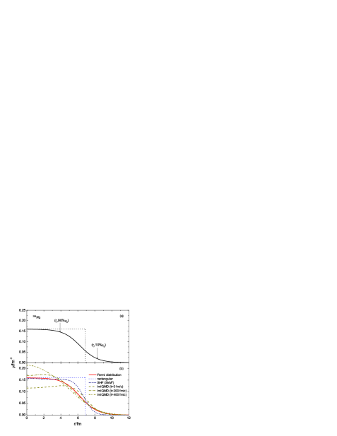
Figure 1: Comparisons of the radial density distributions of the Fermi form, rectangular, Skyrme Hartree-Fock (SHF) with SkM* parameters and the time evolutions in ImIQMD model.

In the dynamical process of two nuclei approaching, we deal with the shell correction of the colliding system with a switch function method [9, 15] which is used in the classical molecular dynamics simulation [16]. The shell correction energy of the system in the dynamical evolution is written as

$$U_{sh}=\sum_{i=1}^{2}\frac{1+x_{i}}{N_{i}}\sum_{j=1}^{N_{i}}\frac{E_{sh}^{i}}{1+\exp[(\mathbf{r}_{j}-R_{0}^{i})/a]},$$ (21)

where the labels $i,j$ denote the sum over the colliding nuclei and the nucleons of the considering nucleus, respectively. The factors $E_{sh}^{i}$ and $R_{0}^{i}$ are given by

$$E_{sh}^{i}(R)=E_{i}S(R)+E_{c}(1-S(R))$$ (22)

and

$$R_{0}^{i}=R_{i}S(R)+R_{c}(1-S(R))$$ (23)

respectively. Here the $E_{i,c}$ and $R_{i,c}$ are the shell correction energies and the radii for projectile ($i=1$), target ($i=2$) and compound nucleus (c), respectively. The switch function is expressed as

$$S=C_{0}+C_{1}\chi+C_{2}\chi^{2}+C_{3}\chi^{3}+C_{4}\chi^{4}+C_{5}\chi^{5},$$ (24)

where $\chi=\left(\frac{R-R_{cf}}{R_{ci}-R_{cf}}\right)$ and $R$ is the distance of the centers between projectile and target. The quantities $R_{ci}$ and $R_{cf}$ are the distances at the initial time and at the compound nucleus formation. In the calculation, we set $R_{ci}=10+R_{1}+R_{2}$ fm and $R_{cf}=R_{c}-R_{2}$ fm. The coefficients $C_{0}$, $C_{1}$, $C_{2}$, $C_{3}$, $C_{4}$ and $C_{5}$ are taken to be 0, 0, 0, 10, -15 and 6, respectively. Fig. 2 shows the time evolutions of the shell correction energy for the double magic nuclei ⁴⁸Ca and ²⁰⁸Pb using Eq. (19) and in the reaction ⁴⁸Ca+²⁰⁸Pb$\rightarrow$ ²⁵⁶No using Eq. (21). For the single nucleus evolution in ImIQMD model, the calculated shell correction energies approach the empirical formula [14] (-5.48 MeV for ⁴⁸Ca and -8.93 MeV for ²⁰⁸Pb). In the approaching process of two colliding nuclei, the shell correction energy of the system evolves from the sum of projectile and target to the one of the compound nucleus.

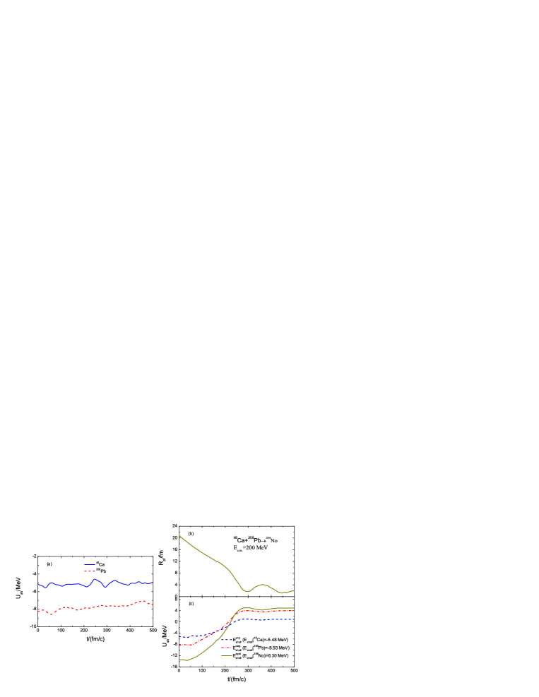
Figure 2: The time evolutions of the shell correction energies for the double magic nuclei ⁴⁸Ca and ²⁰⁸Pb (a), the distance of centers between projectile and target (b) and the shell correction energies of projectile, target and system in the reaction ⁴⁸Ca+²⁰⁸Pb$\rightarrow$ ²⁵⁶No (c) at the incident center-of-mass (c.m.) energy 200 MeV.

The phase space constraint method is also introduced in the ImIQMD model, which is proposed by Papa et al. in order to improve the nucleon’s fermionic nature [17]. The one-body occupation probability is given by

$$\overline{f}_{i}=\sum_{j}\delta_{s_{i}s_{j}}\delta_{\tau_{i}\tau_{j}}\int_{h^{3}}f_{j}(\mathbf{r},\mathbf{p},t)d\mathbf{r}d\mathbf{p},$$ (25)

where the quantities $s_{i}$ and $\tau_{i}$ represent the quantum numbers of spin and isospin for the $i$th nucleon, respectively. The integration is performed within the phase space volume $h^{3}$ at the center position $\mathbf{r_{i}},\mathbf{p_{i}}$. In the dynamical evolution, we timely examine the occupation probability with the condition $\overline{f}_{i}\leq 1$. Otherwise, a series of two-body scattering are performed to reduce the phase space occupation probability.

The main difficulties of the usual QMD and IQMD model in the description of heavy-ion fusion reactions near Coulomb barrier are to construct a stable nucleus over the reaction time of the compound nucleus formation (typically 10^-21 $\sim$ 10^-20 s). For that Maruyama et al. proposed a cooling method in the study of the fusion reaction ¹⁶O+¹⁶O [18]. The stability of a single nucleus is obviously improved in the ImIQMD model. We give an examination of the root-mean-square radii and the average binding energies for the magic nuclei as shown in Fig. 3. The stabilities maintain 800 fm/c for the selected nuclei. It is necessary for investigating the fusion dynamics of light and intermediate nuclei or the capture process of heavy colliding systems. For the complete fusion of heavy systems, especially the synthesis of superheavy nuclei, or the damped reactions of two very heavy colliding nuclei [19], the stability of the single nucleus needs to be keep longer time.

Figure 3: The time evolutions of the root-mean-square radii and the average binding energies for the magic nuclei ¹⁶O, ⁴⁸Ca, ⁹⁰Zr, ¹³²Sn and ²⁰⁸Pb.

3 Results and discussions

In this section the ImIQMD model is applied to analyze the fusion dynamics at energies near Coulomb barrier. It is well known that the enhancement of the sub-barrier fusion cross sections is related to the various couplings of the relative motion to the nuclear shape vibrations, deformations and nuclear transfer degrees of freedom. The fusion barrier at various energies and the dynamical barrier distribution are investigated systematically using the ImIQMD model. The influence of the shell effect on the fusion cross sections is analyzed. The fusion and capture excitation functions for a series of reaction systems are calculated and compared them with experimental data.

3.1 Fusion barrier and dynamical barrier distribution

The interaction potential $V(R)$ of two colliding nuclei as a function of the distance $R$ between their centers is defined as [20]

$$V(R)=E_{pt}(R)-E_{p}-E_{t}.$$ (26)

Here the $E_{pt}$, $E_{p}$ and $E_{t}$ are the total energies of the whole system, projectile and target, respectively. The total energy is the sum of the kinetic energy, the effective potential energy and the shell correction energy. In the calculation, the Thomas-Fermi approximation is adopted for evaluating the kinetic energy [9]. The static and dynamical interaction potentials are calculated according to Eq. (26) as shown in Fig. 4 for head on collisions of the reaction systems ⁴⁸Ca+²³⁸U and ³⁶S+^90,96Zr. The static interaction potential means that the density distribution of projectile and target is always assumed to be the same as that at initial time, which is a diabatic process and depends on the collision orientations and the mass asymmetry of the reaction systems. The total density of the system is taken as the sum of the individual nucleus in the overlapping region. For a comparison, the proximity results [21] and the adiabatic barrier as mentioned in Ref. [22] are also shown in the figure (left panel) and the corresponding barrier heights are indicated for the various cases. However, for a realistic heavy-ion collision, the density distribution of the whole system will evolve with the reaction time, which significantly depends on the incident energy and impact parameter for a given system. In the calculation of the dynamical potentials, we only pay attention to the fusion events as shown later, which give the fusion dynamical barrier. At the same time, stochastic rotation is performed for different simulation events. One can see that the heights of the dynamical barriers are reduced gradually with decreasing the incident energy and increasing the neutron number of the target. The lowering of the dynamical fusion barrier is in favor of the enhancement of the sub-barrier fusion cross sections, which can give a little of information that the cold fusion reactions are also suitable to produce superheavy nuclei. We can understand the microscopic process of the lowering from the neck formation which derives from the nucleon transfer and the dynamical deformation in the fusion reactions [23].

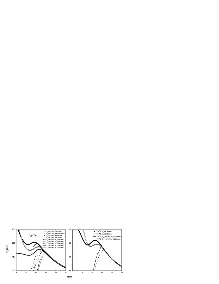
Figure 4: Comparison of the static fusion barriers (including pole-to-pole and waist-to-waist collisions), adiabatic barrier, proximity results and dynamical barriers at different incident c.m. energies for the reaction ⁴⁸Ca+²³⁸U (left panel), as well as system dependence of the static and dynamical fusion barriers (right panel).

The dynamical fusion barrier is calculated by averaging the fusion events at a given energy and an impact parameter. To explore more information on the fusion dynamics, we also investigate the dynamical barrier distribution as shown in Fig. 5 for head on collisions of the reaction ³⁶S+⁹⁰Zr at incident energies 80 MeV and 85 MeV (static barrier $V_{b}=84.37$ MeV), respectively. The distribution moves towards the lower barrier region with decreasing the incident energy. A number of fusion events are located at the sub-barrier region, which is favorable to sub-barrier fusion reactions. Rowley et al. proposed a method of extracting the fusion barrier distribution from the second energy derivative of the fusion excitation function [24]. A portion of the distribution is located at the sub-barrier region from the analysis of experimental fusion excitation functions, which may help us understanding the sub-barrier fusion and the kind of various couplings.

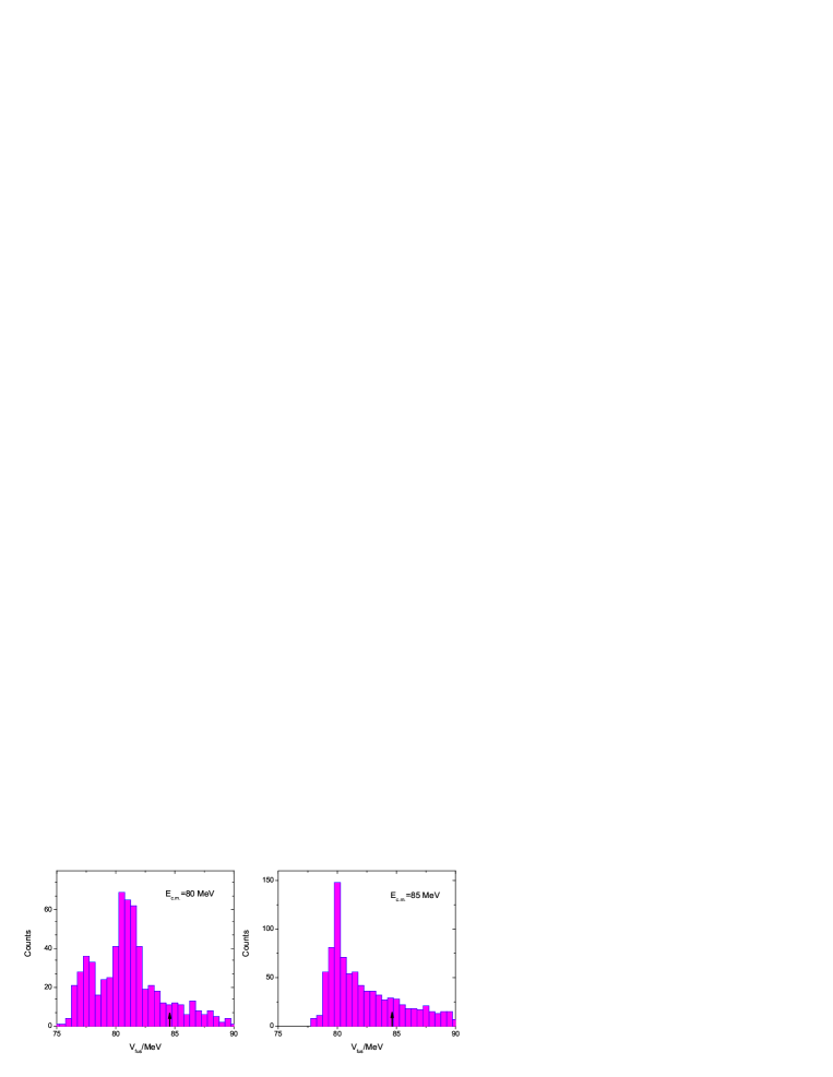
Figure 5: Dynamical barrier distribution for the reaction ³⁶S+⁹⁰Zr at incident energies 80 MeV and 85 MeV, respectively. Arrows show the static fusion barriers.

3.2 Fusion and capture excitation functions

After constructing the stable events of projectile and target, the simulation of the fusion reaction can be performed. Stochastic rotation around their centers of mass for each nucleus by a Euler angle is made for every event at a given incident energy and an impact parameter. The simulation events are set to be 200 for each incident energy $E$ and impact parameter $b$, and be 300 at the sub-barrier energies. The fusion cross section is calculated by the formula

$$\sigma_{fus}(E)=2\pi\int_{0}^{b_{max}}bp_{fus}(E,b)db=2\pi\sum_{b=\Delta b}^{b_{max}}bp_{fus}(E,b)\Delta b,$$ (27)

where $p_{fus}(E,b)$ stands for the fusion probability and is given by the ratio of the fusion events $N_{fus}$ to the total events $N_{tot}$. The reliability of the calculated $p_{fus}(E,b)$ is estimated by the value [18]

$$\Delta P_{f}=1.64\left[\frac{N_{fus}(N_{tot}-N_{fus})}{N_{fus}^{3}}\right]^{1/2}.$$ (28)

In the calculation the step of the impact parameter is set to be $\Delta b=0.5$ fm. We also use the same procedure in the definition of the fusion event in Ref. [7] that the coalesced one-body density can survive through one or more rotations of the composite system or through several oscillations of its radius. The capture cross section of heavy colliding system is also calculated using Eq. (27), in which the capture event is defined as that the distance between the centers of colliding nuclei is smaller than the minimum position of the pocket of the static interaction potential. In Fig. 6 we show the dependence of the fusion probability as a function of the impact parameter on the incident energies in the reaction ³⁶S+⁹⁰Zr and on the system size at the energy $E_{c.m.}$=80 MeV. One can see that the higher incident energy and the neutron-rich system have the larger fusion probability, and the fusion probability is reduced with increasing the impact parameter or the relative angular momentum at each incident energy. There is no signal on the appearance of the so-called ”fusion window” as predicted by the time dependent Hartree-Fock method [25].

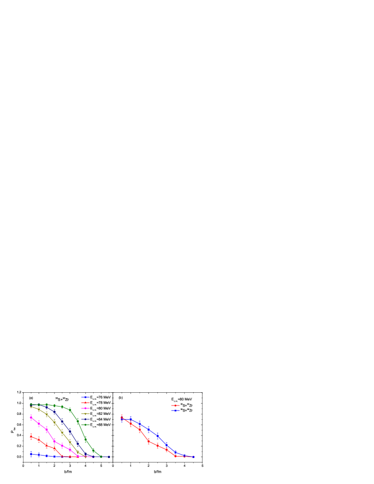
Figure 6: The fusion probability as a function of the impact parameter and its dependence on the incident energies and on the system size.

Recent experimental data showed that there was no enhancement of the fusion cross sections in the reactions ⁴⁸Ca+⁹⁰Zr or ⁹⁶Zr comparing those in the reactions ⁴⁰Ca+⁹⁰Zr or ⁹⁶Zr although using more neutron-rich projectile ⁴⁸Ca [26]. Possible reason is explained from the fact that the double magic nucleus ⁴⁸Ca has more rigid (stronger shell effect) structure than ⁴⁰Ca. We analyzed the influence of the shell effect on the fusion cross sections in the reaction ⁴⁸Ca+⁹⁰Zr as shown in Fig. 7. With the same initial conditions such as the stable event and the distance of the centers between two nuclei etc, the calculated fusion cross sections are obviously reduced after considering the shell correction, especially in the sub-barrier domain. The main reason is that the shell correction potential in Eq. (7) constrains the motion of the surface nucleons of the colliding nuclei. The experimental data can be reproduced rather well by considering the shell correction.

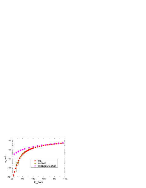
Figure 7: The calculated fusion cross sections with and without considering shell effect in the reaction ⁴⁸Ca+⁹⁰Zr and compared with experimental results [26].

Fig. 8 shows a comparison of the calculated fusion excitation functions by the ImIQMD model after considering the shell correction, one-dimensional Hill-Wheeler formula [27] and the experimental results for the reactions ⁴⁶Ti+⁴⁶Ti [28] and ⁴⁰Ca+¹¹²Sn [29]. The Hill-Wheeler formula underestimates the fusion cross sections at the sub-barrier energies for the two reaction systems. There is no other adjustable parameters in the ImIQMD model, which is a purely dynamical process. The agreement of the calculated fusion excitation functions with the experimental data is remarkably well within statistical error bars. For systematically examining the reliability of the model and exploring the fusion dynamics, we calculated the fusion cross sections of a series of the reaction systems and compared them with available experimental data [26, 30, 31, 32, 33] as shown in Fig. 9. One can see that the neutron-rich combinations have the larger fusion cross section, especially at the sub-barrier regions. As we discussed in the section 3.1, the neutron-rich systems give the lower dynamical fusion barriers at the same incident c.m. energy, which are favorable to increase the fusion cross sections, especially at the sub-barrier energies. The reactions ¹⁸O+⁵⁸Ni and ¹⁶O+⁶⁰Ni lead to the same compound nucleus formation. However, the system ¹⁸O+⁵⁸Ni has the larger fusion cross sections at the sub-barrier energies. Zagrebaev explained the enhancement owing to the positive $Q$ value of the neutron transfer by using a simplified model [34]. Therefore, the colliding system has a little surplus energy to pass over the interaction barrier. In the ImIQMD model, since the magic nucleus ¹⁶O has the stronger shell effect than ¹⁸O, the transfer of the surface nucleon is slightly constrained in the course of projectile and target approaching, which also results in the decrease of the sub-barrier fusion cross sections.

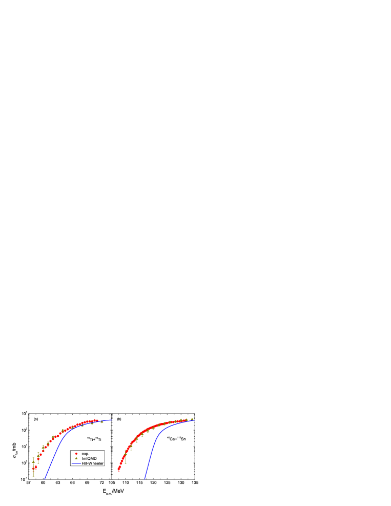
Figure 8: Comparisons of the calculated fusion excitation functions, Hill-Wheeler formula [27] and experimental data [28, 29] for the reactions ⁴⁶Ti+⁴⁶Ti and ⁴⁰Ca+¹¹²Sn.

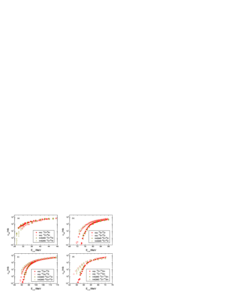
Figure 9: Comparisons of the calculated fusion excitation functions and experimental data for a series of reaction systems.

The synthesis of heavy or superheavy nuclei is mainly reached by the complete fusion reactions of two heavy colliding nuclei in experimentally [35, 36]. In accordance with the evolution of the colliding system, the whole process of the compound nucleus formation and decay is usually divided into three reaction stages, namely the capture process of the colliding system to overcome Coulomb barrier, the formation of the compound nucleus to pass over the inner fusion barrier, and the de-excitation of the excited compound nucleus against fission [37]. As the first stage of synthesizing superheavy nuclei, the accurate calculation of the capture cross sections and the analysis of the capture dynamics are very important to estimate the evaporation residue cross sections and also affect the competition of the complete fusion and the quasi-fission. Within the framework of the ImIQMD model, we analyzed the time evolutions of the relative angular momentum and the distance between the centers of the projectile and target in the ⁴⁸Ca+²³⁸U reaction at incident energy $E_{c.m.}$=200 MeV as shown in Fig. 10. The relative angular momentum is defined as $J=(X_{c.m.}^{p}-X_{c.m.}^{t})\sqrt{2\mu E_{c.m.}}/\hbar$ with the reduced mass of the colliding system $\mu$ and the center of mass distance in the $X$ directions for projectile and target which defines the impact parameter at the initial time. The colliding system evolves from the individual nuclei to the dinuclear system formation, which is a process of the dissipation of the relative angular momentum and the kinetic energy of the relative motion. In Fig. 11 we present a comparison of the calculated capture cross sections and the experimental data for a series of reaction systems. The experimental data are taken from Refs. [38, 39, 40, 41]. One can see that the calculated results are in good agreement with the experimental data. Fig. 12 also shows the calculated capture excitation functions for the reactions ⁴⁸Ca+²⁴⁴Pu and ⁴⁸Ca+²⁴⁸Cm and compared them with available experimental data [42], which have been used to synthesize superheavy elements Z=114 and Z=116 in Dubna [43]. Here, we have considered the quadrupole deformation for the deformed nucleus at the initial sampling. The capture process of the considered systems takes place in the evolution range t=600-800 fm/c. Then, the composite system evolves into either separating two fragments with a larger probability (quasi-fission) or maintaining a whole system with a smaller probability which leads to the compound nucleus formation. It needs a longer evolution time and the larger simulation events to investigate the quasi-fission and the complete fusion in the two heavy colliding nuclei. Further works are in progress.

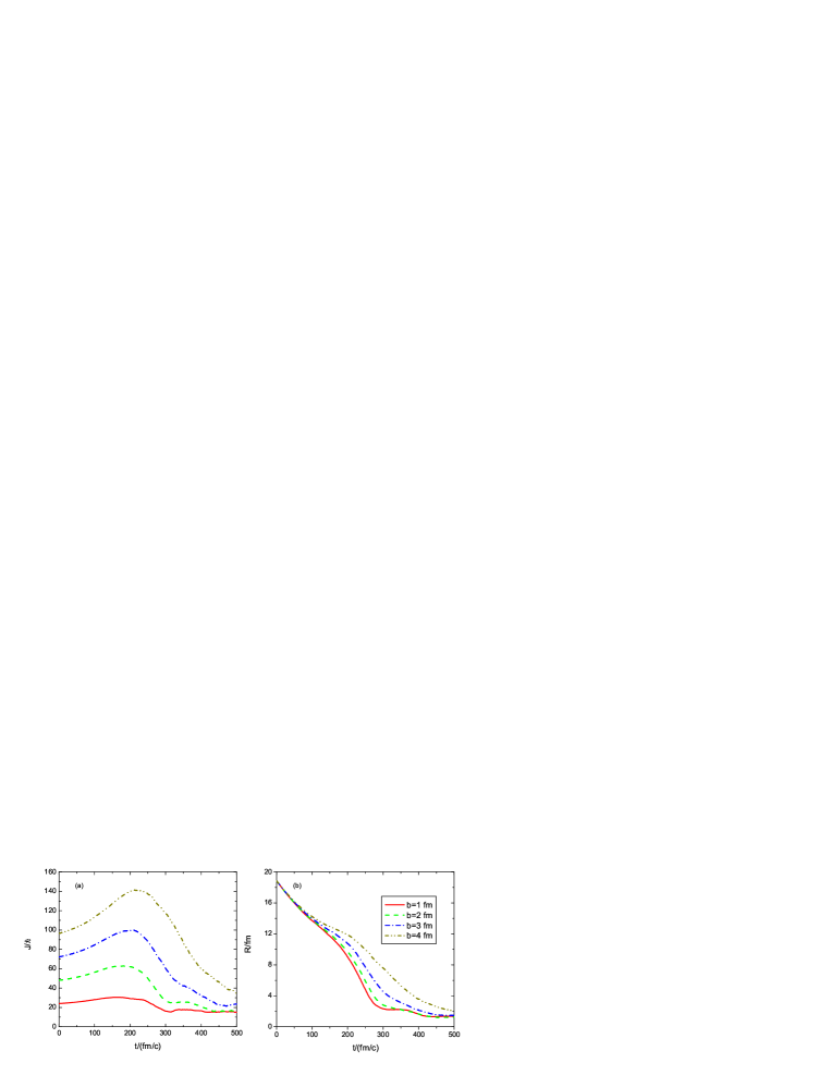
Figure 10: The time evolutions of the relative angular momentum and the distance between the centers of two colliding nuclei in the reaction ⁴⁸Ca+²³⁸U at incident energy 200 MeV.

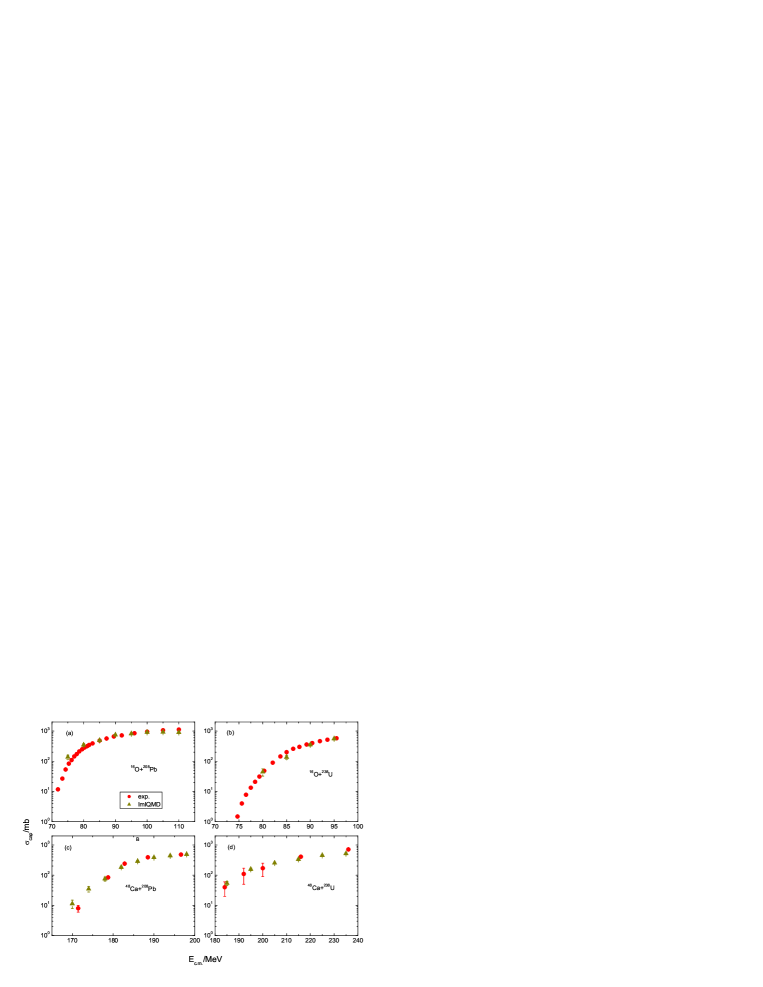
Figure 11: Comparisons of the calculated capture excitation functions and experimental data for the selected reaction systems.

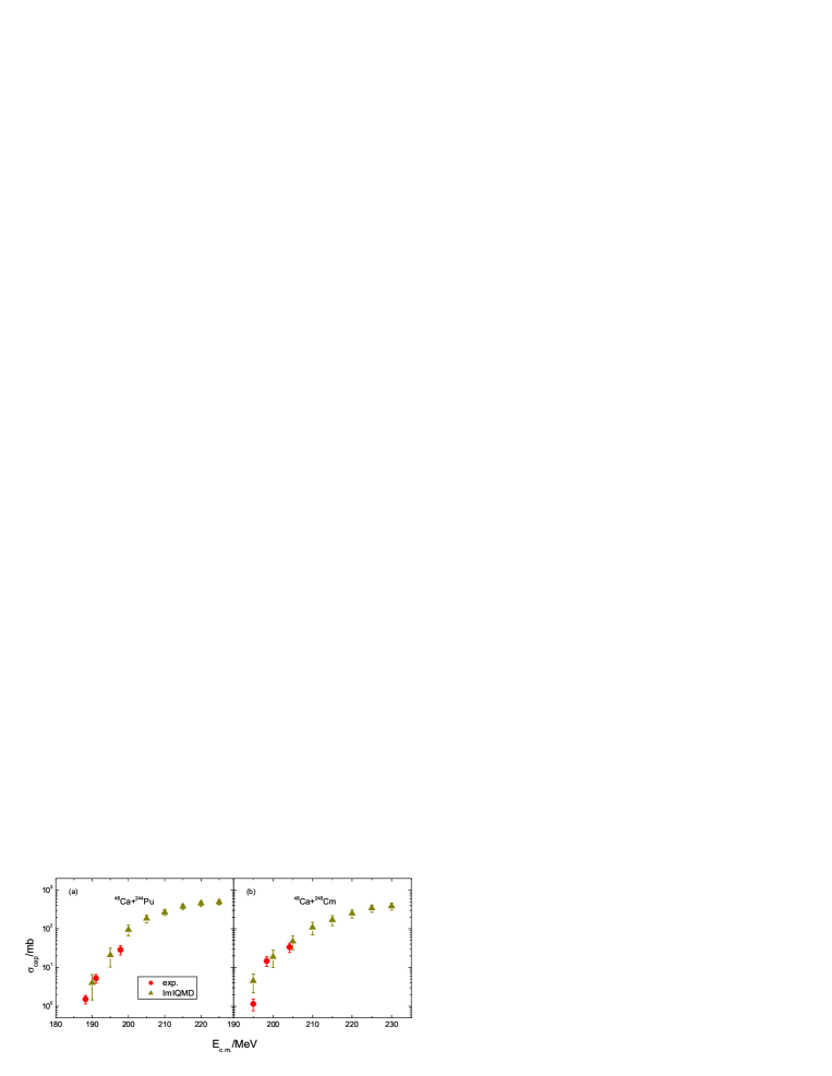
Figure 12: The calculated capture excitation functions for the reactions ⁴⁸Ca+²⁴⁴Pu and ⁴⁸Ca+²⁴⁸Cm and compared them with available experimental data [42].

4 Conclusions

The shell correction has been further considered in the ImIQMD model. Its influence on the fusion excitation functions is analyzed and compared with the experimental data. By using the ImIQMD model, the fusion dynamics in heavy-ion collisions near Coulomb barrier is investigated systematically, such as the fusion barrier, dynamical barrier distribution etc. The calculated excitation functions of the fusions and captures are in good agreement with the available experimental data. The lowering of the dynamical fusion barrier favors the enhancement of the sub-barrier fusion cross sections. The strong shell effect constrains the fusion of two colliding nuclei at near barrier energies.

The physical nature of the heavy-ion fusion reactions near Coulomb barrier is very complicated, which is a dynamical process involving the excitation of the colliding system. Semi-classical dynamical model can explore its dynamical behavior in a certain extent. There are also some interesting works applying the ImIQMD model to investigate the halo nucleus induced reactions, the fusion dynamics (capture, quasi-fission and complete fusion) of the synthesis of the superheavy nuclei in the massive fusion reactions, and searching other possible ways to produce superheavy nuclei etc. For those cases, the structure properties and the longer stability of the initial nucleus have to be made.

5 Acknowledgements

One of us (Z.Q. Feng) is grateful to Profs. Zhuxia Li, Junqing Li, Werner Scheid, Hans Feldmeier and Dr. Ning Wang for fruitful discussions and help, and also thanks the hospitality during his stay in GSI. This work was supported by the National Natural Science Foundation of China under Grant No. 10475100, the Major state basic research development program under Grant No. 2007CB815000, and the Helmholtz-DAAD in Germany.

References

- [1] A.B. Balantekin, N. Takigawa, Rev. Mod. Phys. 70 (1998) 77.
- [2] J. Aichelin, Phys. Rep. 202 (1991) 233.
- [3] E.A. Uehling, G.E. Uhlenbeck, Phys. Rev. 43 (1933) 552.
- [4] L.W. Chen, F.S. Zhang, G.M. Jin, Phys. Rev. C 58 (1998) 2283.
- [5] F.S. Zhang, L.W. Chen, Z.Y. Ming, Z.Y. Zhu, Phys. Rev. C 60 (1999) 064604.
- [6] B.A. Li, C.M. Ko, W. Bauer, Int. J. Mod. Phys. E 7 (1998) 147.
- [7] N. Wang, Z.X. Li, X.Z. Wu, Phys. Rev. C 65 (2002) 064608; N. Wang, X.Z. Wu, Z.X. Li, Phys. Rev. C 67 (2003) 024604; N. Wang, Z.X. Li, X.Z. Wu, et al., Phys. Rev. C 69 (2004) 034608.
- [8] T. Neff, H. Feldmeier, K. Langanke, arXiv: nucl-th/0703030.
- [9] Z.Q. Feng, F.S. Zhang, G.M. Jin, X. Huang, Nucl. Phys. A 750 (2005) 232.
- [10] Ch. Hartnack, R.K. Puri, J. Aichelin, et al., Eur. Phys. J. A 1 (1998) 151.
- [11] M. Brack, C. Guet, H.-B. Hakansson, Phys. Rep. 123 (1985) 275.
- [12] E. Chabanat, P. Bonche, P. Haensel, et al., Nucl. Phys. A 627 (1997) 710; Nucl. Phys. A 635 (1998) 231; Nucl. Phys. A 643 (1998) 441 (erratum).
- [13] Y.X. Zhang, Z.X. Li, Phys. Rev. C 74 (2006) 014602.
- [14] G. Royer, B. Remaud, J. Phys. G 10 (1984) 1057.
- [15] Z.Q. Feng, F.S. Zhang, W.F. Li, G.M. Jin, High Ener. Phys. Nucl. Phys., 29 (2005) 41.
- [16] An.R. Leach, Molecular Modelling (Principles and Applications), 1st edition (World Press Corporation, Beijing, 1996).
- [17] M. Papa, T. Maruyama, A. Bonasera, Phys. Rev. C 64 (2001) 024612.
- [18] T. Maruyama, A. Ohnishi, H. Horiuchi, Phys. Rev. C 42 (1990) 386.
- [19] N. Wang, Z.X. Li, X.Z. Wu, E.G. Zhao, Mod. Phys. Lett. A 20 (2005) 2619.
- [20] K.A. Brueckner, J.R. Buchler, M.M. Kelly, Phys. Rev. 173 (1968) 944.
- [21] W.D. Myers, W.J. Swiatecki, Phys. Rev. C 62 (2000) 044610.
- [22] K. Siwek-Wilczynska, J. Wilczynski, Phys. Rev. C 64 (2001) 024611.
- [23] Z.Q. Feng, G.M. Jin, F.S. Zhang, et al., Chin. Phys. Lett. 22 (2005) 3040.
- [24] N. Rowley, G.R. Satchler, P.H. Stelson, Phys. Lett. B 254 (1991) 25.
- [25] C.Y. Wong, Phys. Rev. C 25 (1982) 1460.
- [26] A.M. Stefanini, F. Scarlassara, S. Beghini, et al., Phys. Rev. C 73 (2006) 034606.
- [27] D.L. Hill, J.A. Wheeler, Phys. Rev. 89 (1953) 1102.
- [28] A.M. Stefanini, M. Trotta, L. Corradi, et al., Phys. Rev. C 65 (2002) 034609.
- [29] F. Scarlassara, S. Beghini, G. Montagnoli, et al., Nucl. Phys. A 672 (2000) 99.
- [30] A.M. Borges, C.P. da Silva, D. Pereira, et al., Phys. Rev. C 46 (1992) 2360.
- [31] A.M. Stefanini, L. Corradi, A.M. Vinodkumar, et al., Phys. Rev. C 62 (2000) 014601.
- [32] C.R. Morton, M. Dasgupta, D.J. Hinde, et al., Phys. Rev. Lett. 72 (1994) 4074.
- [33] J.X. Wei, J.R. Leigh, D.J. Hinde, et al., Phys. Rev. Lett. 67 (1991) 3368.
- [34] V.I. Zagrebaev, Phys. Rev. C 67 (2003) R061601.
- [35] S. Hofmann, G. Münzenberg, Rev. Mod. Phys. 72 (2000) 733; S. Hofmann, Rep. Prog. Phys. 61 (1998) 639.
- [36] Yu.Ts. Oganessian, J. Phys. G34 (2007) R165; Nucl. Phys. A 787 (2007) 343c.
- [37] Z.Q. Feng, G.M. Jin, F. Fu, J.Q. Li, Nucl. Phys. A 771 (2006) 50; Z.Q. Feng, G.M. Jin, J.Q. Li, W. Scheid, Phys. Rev. C 76 (2007) 044606.
- [38] M. Dasgupta, D.J. Hinde, Nucl. Phys. A 734 (2004) 148.
- [39] K. Nishio, H. Ikezoe, Y. Nagame, et al., Phys. Rev. Lett. 93 (2004) 162701.
- [40] E.V. Prokhorova, E.A. Cherepanov, M.G. Itkis, et al., arXiv: nucl-ex/0309021.
- [41] W.Q. Shen, J. Albinski, A. Gobbi, et al., Phys. Rev. C 36 (1987) 115.
- [42] M.G. Itkis, J. Äystö, S. Beghini, et al., Nucl. Phys. A 734 (2004) 136.
- [43] Yu.Ts. Oganessian, V.K. Utyonkov, Yu.V. Lobanov, et al., Phys. Rev. C 62 (2000) R041604; Phys. Rev. C 63 (2001) R011301.