Remote controlled-NOT gate of $d$-dimension

Abstract

Single qubit rotation gate and the controlled-NOT (CNOT) gate constitute a complete set of gates for universal quantum computation. In general the CNOT gate is only for two nearby qubits. For two qubits which are remote from each other, we need a series of swap gates to transfer these two qubits to the nearest neighboring sites, and then after the CNOT gate we should transfer them to their original sites again. However, a series of swap gates are resource for quantum information processing. One economy way which does not consume so much resource is to implement CNOT gate remotely. The remote CNOT gate is to implement the CNOT gate for two remotely separated qubits with the help of one additional maximally entangled state. The original remote CNOT gate is for two qubits, here we will present the $d$-dimensional remote CNOT gate. The role of quantum teleportation is identified in the process of the remote CNOT gate.

Quantum information and quantum computation have been attracting a great deal of interests in the past years since some computing tasks can be sped up on a quantum computer CNOT .

To perform the universal quantum computation, we only need several elementary gates to be implemented BBCD . For example, the single qubit rotation gate and the controlled-NOT (CNOT) gate constitute a complete set of gates for universal quantum computation. The CNOT gate is a two-qubit gate which involves a global unitary transformation on two qubits coherently, and it can not be realized individually on two qubits separately. This is because that actually CNOT gate can create a maximally entangled state from a product (thus separate) state and it is nonlocalremote CNOT . In real quantum systems, the qubits only interact with each other when they are in nearest neighboring sites. It is not free to move one qubit from one site to another site, which means the quantum state transfer is not free in real quantum systems. Compared with a quantum system where the quantum state can be transferred freely, extra error penalty should be paid for the fault tolerant quantum computation with only nearest neighboring communication SBF . Thus to implement a CNOT gate on two qubits, we should assume that these two qubits are in nearest neighboring sites so that they can interact with each other and in this way the CNOT gate realization is possible. To move one qubit from one-site to another, we need a series of swap gates, each of them swap two nearest neighboring qubits. The swap gate can be realized by several CNOT and single-qubit rotation gates. However, this scheme can be considered to be resource consuming since we generally want the quantum circuit involving only a small amount of quantum gates. One way to solve this problem is to transfer quantum state through a quantum bus as demonstrated recently in experiments bus1 ; bus2 . In this paper, we will consider another way which is to construct a remote CNOT gate with the expense of a prior maximally entangled state H Representation ; gottesman ; DK ; remote CNOT ; remote CNOT1 ; remote CNOT2 ; remote CNOT3 ; remote CNOT4 . The advantages of the remote CNOT gate are, for example: the remote CNOT involves only a few quantum gates and thus the error rate will be low; we only need to concern about how well the quality of the shared entangled state is, and we do not need to care too much the decoherence in the chain of qubits. While the remote CNOT gate is only for two-qubit system, the $d$-dimensional remote CNOT gate is still absent. In this paper, we will present the form of the general remote CNOT gate in $d$-dimensional quantum system. And the role of quantum teleportation is identified explicitly in this remote CNOT gate.

One of the most amazing protocols in quantum information processing is the well-known quantum teleportation teleportation . In quantum teleportation, a quantum state can be transferred from one place to another place by only local operations and classical communication when a prior maximally entangled state is shared between these two spatially separated parties. It is not only useful in quantum information transfer, but also primitive in the universal quantum computation, for example, if the quantum teleportation can be realized, then the universal quantum computation can be achieved with only measurements GC .

In the quantum teleportation demonstrated in Ref.teleportation , to teleport the unknown state of qubit $A^{\prime}$, Alice needs to perform a Bell measurement on qubits $A$ and $A^{\prime}$. Then Alice tells Bob the result of her measurement through classical channel. Bob takes corresponding operation on qubit $B$ to obtain the state of $\left|\phi\right\rangle_{B}$. We would like to remark that so far, Bell measurement is not easy to be performed experimentally Bell measurement1 ; Bell measurement2 ; Bell measurement3 . However, with CNOT gate available, the teleportation without Bell measurement can be performed H Representation . Unlike Bell measurement, Alice only needs to measure the two individual qubits in their computational basis respectively. In this scheme, CNOT play an nontrivial role because CNOT can change entangled states into product states. On the other hand, as is well known, it also has the entanglement power.

In this paper, we will firstly show that the $d$-dimensional CNOT gate plays a same role in the $d$-dimensional single-qudit measurement quantum teleportation (hereafter, the $d$-dimensional state is named as qudit to correspond the qubit for two-dimensional quantum state), which is helpful to understand its application in remote CNOT of $d$-dimension. Then, by generalizing the remote CNOT in two-dimension to higher dimension, we present the remote CNOT in $d$-dimensional Hilbert space. And the relation between teleportation and remote CNOT are discussed.

To begin with, let’s introduce some notations. In $d$-dimensional Hilbert space, $U_{mn}=X^{m}Z^{n}$ $\left(m,n=0,1\ldots,d-1\right)$ are generalized Pauli matrices constituting a basis of unitary operators, and $X\left|j\right\rangle=\left|\left(j+1\right)\text{mod}d\right\rangle$, $Z\left|j\right\rangle=e^{i2\pi j/d}\left|j\right\rangle$, where $\left\{\left|j\right\rangle\right\}_{j=0}^{d-1}$ is an orthonormal basis. The generalized CNOT operator and Hadamard operator are $C_{01}=\overset{d-1}{\underset{j,k=0}{\sum}}\left|j\right\rangle_{0}\left\langle j\right|\otimes\left|k+j\right\rangle_{1}\left\langle k\right|$ and $H=\frac{1}{\sqrt{d}}\overset{d-1}{\underset{j,k=0}{\sum}}e^{i2\pi jk/d}\left|k\right\rangle\left\langle j\right|$. State at site $0$ is the control-qudit, state at site 1 is the target-qudit. Arbitrary single-qudit state in $d$-dimensional Hilbert space can be expressed as

$$\left|\phi\right\rangle_{0}=\overset{d-1}{\underset{j=0}{\sum}}a_{j}\left|j\right\rangle_{0},$$ (1)

where $\overset{d-1}{\underset{j=0}{\sum}}\left|a_{j}\right|^{2}=1$. Let Alice and Bob share an maximally entangled state

$$\left|\Psi^{\left(0\right)}\right\rangle_{12}=\frac{1}{\sqrt{d}}\overset{d-1}{\underset{j=0}{\sum}}\left|jj\right\rangle_{12}.$$ (2)

Here qudits 0 and 1 hold by Alice and qudit 2 hold by Bob.

Applying the following two gates, we obtain

$$H_{0}C_{01}^{\dagger}\left|\phi\right\rangle_{0}\left|\Psi^{\left(0\right)}\right\rangle_{12}$$ (3)

$$= \frac{1}{\sqrt{d}}\overset{d-1}{\underset{j=0}{\sum}}\overset{d-1}{\underset{j^{\prime}=0}{\sum}}a_{j}\frac{1}{\sqrt{d}}\overset{d-1}{\underset{n=0}{\sum}}e^{i2\pi jn/d}\left|n\right\rangle_{0}\left|j^{\prime}-j\right\rangle_{1}\left|j^{\prime}\right\rangle_{2}.$$

Here $C_{01}^{\dagger}$ is the conjugate operator of $C_{01}$, and explicitly $C_{01}^{\dagger}=\overset{d-1}{\underset{j,k=0}{\sum}}\left|j\right\rangle_{0}\left\langle j\right|\otimes\left|k-j\right\rangle_{1}\left\langle k\right|$. For $d=2$ case, we have $C_{01}^{\dagger}=C_{01}$, however, $C_{01}^{\dagger}\neq C_{01}$ when $d>2$. By inserting identity $I_{1}=\overset{d-1}{\underset{m=0}{\sum}}\left|m\right\rangle_{1}\left\langle m\right|$ into Eq.(3) and straightforward calculating, we have

$$H_{0}C_{01}^{\dagger}\left|\phi\right\rangle_{0}\left|\Psi^{\left(0\right)}\right\rangle_{12}=\frac{1}{d}\overset{d-1}{\underset{n=0}{\sum}}\overset{d-1}{\underset{m=0}{\sum}}\left|n\right\rangle_{0}\left|m\right\rangle_{1}X^{m}Z^{n}\left|\phi\right\rangle_{2}.$$ (4)

Now it is interesting to note that when qudits 0 and 1 are in computational basis $|n\rangle_{0},|m\rangle_{1}$, qudit 2 is the state $X^{m}Z^{n}|\phi_{0}\rangle$. Apparently, by performing single-qudit measurement on qudits 0 and 1 in computational basis, Alice can get $d^{2}$  possible results with equal probability $\frac{1}{d^{2}}$. According to Alice’s measurement result, Bob then applies corresponding operator $(X^{m}Z^{n})^{\dagger}$ on qudit 2, Bob’s final state is the original state $|\phi\rangle$. That is to say, if Alice gets $\left|n\right\rangle_{0}\left|m\right\rangle_{1}$ by measurement, Bob can recover the state $\left|\phi\right\rangle_{2}$ on qudit 2 by applying corresponding unitary transformation $(X^{m}Z^{n})^{\dagger}$. This is in principle the quantum teleportation in $d$-dimensional Hilbert space. The only difference between this scheme and the original one in Ref.teleportation is that the generalized Bell measurement in $d$-dimension is replaced by a generalized CNOT and Hadamard operation followed by two single-qudit measurement performed only by Alice, i.e., it is still a local operation. The classical communication is certainly necessary to ensure that Bob can recover the teleported state. We remark that when $d=2$, it reduces to the case of qubit teleportation. This teleportation scheme is depicted in the Fig.1.

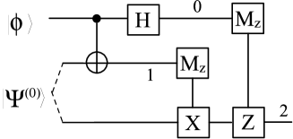
Figure 1: In the teleportation, the Bell measurement by Alice is replaced by a CNOT gate and a Hadarmard gate. The measurement is performed on individual qubits 0 and 1, and the measurement results is communicated through classical channel. According to the measurement results, Bob applies corresponding unitary transformations on 2 to recover the initial state. For $d$-dimensional case, the procedures are almost the same, however, to recover the initial state, the applied matrices on state 2 are the generalized Pauli matrices $(X^{m}Z^{n})^{\dagger}$ corresponding to the measurement results $m,n$ on states $0$ and $1$.

Actually there are another scheme to realize single-qubit measurement teleportation, which is similar to the method discussed in above. Here we just give the direct calculating result as follows,

$$H_{1}C_{10}^{\dagger}\left|\phi\right\rangle_{0}\left|\Psi^{\left(0\right)}\right\rangle_{12}=\frac{1}{d}\overset{d-1}{\underset{n=0}{\sum}}\overset{d-1}{\underset{m=0}{\sum}}\left|n\right\rangle_{0}\left|m\right\rangle_{1}Z^{m}X^{-n}\left|\phi\right\rangle_{2}.$$ (5)

In $d$-dimensional Hilbert space, $X^{-1}\left|j\right\rangle=\left|\left(j-1\right)\text{mod}d\right\rangle$ and $X^{-1}\neq X$ when $d\neq 2$. The only difference between this scheme and the scheme in (4) is that here the controlled qudit and the target qudit exchanged with each other.

As we mentioned, in real physical systems, CNOT gate usually can only be performed for nearby two particles. However, restricted to condition that the particles interaction is only available for nearest neighboring sites, if we have a prior maximally entangled state, CNOT gate for remotely separated particles can be still realized. This remote CNOT for qubits case has already been studied, for example in Ref.gottesman ; H Representation and the remote controlled phase gate which is equivalent to remote CNOT by local operation in Ref.DK . However, the remote CNOT for general $d$-dimensional states is not yet available. We will next present the remote CNOT gate for $d$-dimensional case. For completeness, let’s first consider the remote CNOT in two-dimension.

In two-dimensional Hilbert space, arbitrary quantum state of two qubits, which may be product state or coherent state, can be written as

$$\left|\psi\right\rangle_{ij}=\alpha_{00}\left|00\right\rangle_{ij}+\alpha_{01}\left|01\right\rangle_{ij}+\alpha_{10}\left|10\right\rangle_{ij}+\alpha_{11}\left|11\right\rangle_{ij},$$ (6)

where $\left|\alpha_{00}\right|^{2}+\left|\alpha_{01}\right|^{2}+\left|\alpha_{10}\right|^{2}+\left|\alpha_{11}\right|^{2}=1$. We have already known the CNOT operator $C_{ij}=\left|0\right\rangle_{i}\left\langle 0\right|\otimes I_{j}+\left|1\right\rangle_{i}\left\langle 1\right|\otimes X_{j}$, and then after performing CNOT on state $\left|\psi\right\rangle_{ij}$, we have

$$C_{ij}\left|\psi\right\rangle_{ij}=\alpha_{00}\left|00\right\rangle_{ij}+\alpha_{01}\left|01\right\rangle_{ij}+\alpha_{10}\left|11\right\rangle_{ij}+\alpha_{11}\left|10\right\rangle_{ij}.$$ (7)

Here $i$ denotes control-qubit and $j$ denotes target-qubit.

Now suppose qubits $i$ and $j$ are located remotely, then we can not perform CNOT between them directly. On the other hand, qubit $i^{\prime}$ is in the nearest neighboring site with qubit $i$, similarly qubits $j,j^{\prime}$ are in nearest neighboring sites. Then CNOT gates can be performed directly on pairs $(i,i^{\prime})$ and $(j,j^{\prime})$. And moreover, we suppose that $i^{\prime}$ and $j^{\prime}$ share a maximally entangled state $\left|\Psi^{\left(0\right)}\right\rangle_{i\prime j\prime}=\frac{1}{\sqrt{2}}\left(\left|00\right\rangle_{i\prime j\prime}+\left|11\right\rangle_{i\prime j\prime}\right)$. Let’s consider that states $i,i^{\prime}$ belong to Alice, and $j,j^{\prime}$ belong to Bob. Here in order to see the role of teleportation in the remote CNOT, we divide the scheme of remote CNOT gate into several steps. Step 1, Bob applies CNOT operator $C_{j\prime j}$ on pair $(j,j^{\prime})$locally, then performs Hadamard gate operate on $j^{\prime}$. Thus we have

$$H_{j\prime}C_{j\prime j}\left(\left|\psi\right\rangle_{ij}\otimes\left|\Psi^{\left(0\right)}\right\rangle_{i\prime j\prime}\right)$$ (8)

$$= \frac{1}{2}\left[\left|\psi\right\rangle_{ii^{\prime}}\left|00\right\rangle_{j\prime j}+X_{i^{\prime}}\left|\psi\right\rangle_{ii^{\prime}}\left|01\right\rangle_{j\prime j}\right.$$

$$\left.+Z_{i^{\prime}}\left|\psi\right\rangle_{ii^{\prime}}\left|10\right\rangle_{j\prime j}+Z_{i^{\prime}}X_{i^{\prime}}\left|\psi\right\rangle_{ii^{\prime}}\left|11\right\rangle_{j\prime j}\right].$$

Obviously, this is the same as the teleportation operation as we presented, which can teleport $\left|\psi\right\rangle_{ij}$ to $\left|\psi\right\rangle_{ii^{\prime}}$. Step 2, Alice applies CNOT operator on her side $C_{ii^{\prime}}$. By these two steps, the initial joint state becomes

$$C_{ii\prime}H_{j\prime}C_{j\prime j}\left(\left|\psi\right\rangle_{ij}\otimes\left|\Psi^{\left(0\right)}\right\rangle_{i\prime j\prime}\right)$$

$$= \frac{1}{2}\left[C_{ij}\left|\psi\right\rangle_{ij}\otimes\left|00\right\rangle_{i\prime j\prime}+Z_{i}C_{ij}\left|\psi\right\rangle_{ij}\otimes\left|01\right\rangle_{i\prime j\prime}\right.$$

$$\left.+X_{j}C_{ij}\left|\psi\right\rangle_{ij}\otimes\left|10\right\rangle_{i\prime j\prime}-Z_{i}X_{j}C_{ij}\left|\psi\right\rangle_{ij}\otimes\left|11\right\rangle_{i\prime j\prime}\right].$$

Now we may notice that the states of $i,j$ in each term of the superposition are always related with CNOT gate of $|\psi\rangle$. Step 3, Alice and Bob measures qubit $i^{\prime}$ and $j^{\prime}$ at their own sites in computational basis respectively. By measurement, they can have four results $\left|00\right\rangle$, $\left|01\right\rangle$, $\left|10\right\rangle$ and $\left|11\right\rangle$, each occurs with probability $\frac{1}{4}$. Step 4, by exchanging the classical information of measurement results, Alice and Bob can apply corresponding Pauli operators on qubit $i$ and $j$ respectively. Thus the CNOT gate $C_{ij}$ is realized between remotely separated qubit $i$ and qubit $j$. This is the remote CNOT gate. This processing is depicted in Fig.2

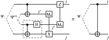
Figure 2: The remote CNOT gate is constituted by two CNOT gates which are performed on nearby qubits or qudits and the Hadamard gates. After the measurement in computational basis represented by $M_{z}$, Alice and Bob in sites $i$ and $j$ apply corresponding transformation according to the measurement results, the CNOT gate is finally realized for remotely separated parties $i$ and $j$. The dashed square part in the scheme is the same as that of the teleportation. Similarly, the $d$-dimensional remote CNOT gate can be realized where the generalized Pauli matrices should be applied according to the measurement results.

Now, we shall present our result of the $d$-dimensional remote CNOT gate. In above, we have already defined some operators in $d$-dimensional Hilbert space, we shall now use them here again. Arbitrary state of two qudits in $d$-dimensional Hilbert space can be expressed as

$$\left|\psi\right\rangle_{ij}=\overset{d-1}{\underset{k,l=0}{\sum}}\alpha_{kl}\left|kl\right\rangle_{ij},$$ (10)

where $\overset{d-1}{\underset{k,l=0}{\sum}}\left|\alpha_{kl}\right|^{2}=1$. Also let $i$ be the control-qudit and $j$ the target-qudit, the CNOT gate is represented as,

$$C_{ij}\left|\psi\right\rangle_{ij}=\overset{d-1}{\underset{k,l=0}{\sum}}\alpha_{kl}\left|k\left(l+k\right)\right\rangle_{ij}.$$ (11)

A prior maximally entangled state shared between Alice and Bob can be written as

$$\left|\Psi^{\left(0\right)}\right\rangle_{i^{\prime}j^{\prime}}=\frac{1}{\sqrt{d}}\overset{d-1}{\underset{m=0}{\sum}}\left|mm\right\rangle_{i^{\prime}j^{\prime}}.$$ (12)

Following the same steps as in two-dimensional remote CNOT case, we obtain

$$C_{ii^{\prime}}H_{j^{\prime}}C_{j^{\prime}j}\left|\psi\right\rangle_{ij}\otimes\left|\Psi^{\left(0\right)}\right\rangle_{i^{\prime}j^{\prime}}$$ (13)

$$= \frac{1}{\sqrt{d}}\overset{d-1}{\underset{m=0}{\sum}}\overset{d-1}{\underset{k,l=0}{\sum}}\alpha_{kl}\left|k\left(l+m\right)\right\rangle_{ij}\otimes\left|\left(m+k\right)\right\rangle_{i^{\prime}}$$

$$\otimes\frac{1}{\sqrt{d}}\overset{d-1}{\underset{n=0}{\sum}}e^{\frac{2\pi inm}{d}}\left|n\right\rangle_{j^{\prime}}$$

$$= \frac{1}{d}\overset{d-1}{\underset{m=0}{\sum}}\overset{d-1}{\underset{n=0}{\sum}}e^{\frac{2\pi inm}{d}}Z_{i}^{-n}X_{j}^{m}C_{ij}^{\dagger}\left|\psi\right\rangle_{ij}\otimes\left|mn\right\rangle_{i^{\prime}j^{\prime}},$$

where the generalized Hadamard gate $H=\frac{1}{\sqrt{d}}\overset{d-1}{\underset{j,n=0}{\sum}}e^{i2\pi jn/d}\left|n\right\rangle\left\langle j\right|$ is equivalent to quantum Fourier transform, and $C_{ij}\left|kl\right\rangle_{ij}=\left|k\left(l+k\right)\right\rangle_{ij}$, $C_{ij}^{\dagger}\left|kl\right\rangle_{ij}=\left|k\left(l-k\right)\right\rangle_{ij}$, $X_{j}\left|l\right\rangle_{j}=\left|\left(l+1\right)\text{mod}d\right\rangle_{j}$, $Z_{i}\left|k\right\rangle_{i}=e^{i2\pi k/d}\left|k\right\rangle_{i}$. Fortunately, still we may notice that in the superposition, state of $i,j$ in each term is always the CNOT gate on $|\psi\rangle$ though extra generalized Pauli matrices are present in front of it. However, by measurement on sites $i^{\prime},j^{\prime}$, those Pauli matrices can be deleted if we apply the corresponding transformations. Now the scheme is like the following: Alice (Bob) measure qudit $i^{\prime}$ ($j^{\prime}$) at her (his) site in computational basis. They will know the state $|m\rangle_{i^{\prime}},|n\rangle_{j^{\prime}}$, and each will occur with probability $\frac{1}{d^{2}}$. Then Alice and Bob exchange the classical information of measurement results and apply corresponding Pauli operators on qudits $i$ and $j$ respectively. Thus the remote CNOT gate $C_{ij}^{\dagger}$ between spatially separated qudits $i$ and $j$ is realized. We note that in $d$-dimensional Hilbert space the final result which is realized is actually the conjugate operator of remote CNOT gate, i.e., $C_{ij}^{\dagger}=\overset{d-1}{\underset{k,l=0}{\sum}}\left|k\right\rangle_{i}\left\langle k\right|\otimes\left|l-k\right\rangle_{j}\left\langle l\right|$. This, however, can be easily changed by a transformation, i.e., the CNOT and Hadarmad in l.h.s. of (13) are changed to their conjugate forms, and the conjugate CNOT in r.h.s. is changed back to CNOT. The reason that we present this form is that our generalization from two-dimensional case to $d$-dimensional case seems more explicit. When $d=2$, $Z^{-1}=Z$ and $C_{ij}^{\dagger}=C_{ij}=\left|0\right\rangle_{i}\left\langle 0\right|\otimes I_{j}+\left|1\right\rangle_{i}\left\langle 1\right|\otimes X_{j}$, it recovers the Eq.(LABEL:9).

From above, we know that remote CNOT gate can be considered as a combination of teleportation operation and a local CNOT operation. The opposite direction is that a local CNOT can be teleported through a maximally entangled state. For qubit case, the universal quantum gates teleported by optical system has been proposed in Ref.quantum gate . Finally we would like to emphasize that the two local CNOT gates and the measurements in the scheme of Fig.2 can be performed in parallel which can be realized at the same time. This scheme is different from the remote CNOT scheme proposed in Refs. PRA65 ; PRA71 ; ph05 . In their nonlocal operations a state-operator which is named as ”stator” need to be prepared first, then a CNOT and a measurement can be performed. That means the two local CNOT and measurements in their scheme should be performed in time order. In this sense, the scheme presented in this paper has the advantage of parallel in computation. Note that our scheme is also different from the scheme in Ref.remote CNOT .

Restricted to condition that only nearest neighboring interaction is usually available in real systems, CNOT gate can only be performed on nearby quantum states. In case CNOT gate is necessary for remotely separated states, the remote CNOT gate is an ideal choice where an extra maximally entangled state is needed. By observing that the remote CNOT gate is actually a combination of teleportation and a CNOT for qubit system, we successfully formulate the $d$-dimensional remote CNOT gate similarly by a $d$-dimensional teleportation and a CNOT gate. In the scheme of remote CNOT gate, the teleportation by Bell measurement is replaced by single state measurement scheme. Our result can be used not only to realize CNOT remotely, but also it can be used to teleport universal quantum gates. Compared with scheme in which states transfer is realized by a series of swap gates, the remote CNOT scheme can be achieved with the expense of one extra maximally entangled state. Thus it can be considered to be an economy way.

Acknowledgements: HF was supported by ”Bairen” program, NSFC grant (10674162) and ”973” program (2006CB921107).

References

- (1) M.A. Nielsen, I.L. Chuang, Quantum Computation and Quantum Information, Cambridge University Press (2000).
- (2) A. Barenco, C. H. Bennett, R. Cleve, D. P. DiVincenzo, N. Margolus, P. Shor, T. Sleator, J. Smolin, H. Weinfurter, Phys. Rev. A 52 (1995) 3457.
- (3) D. Gottesman, The Heisenberg Representation of Quantum Computers, quant-ph/9807006.
- (4) D. Collins, N. Linden, S. Popescu, Phys. Rev. A 64 (2001) 032302.
- (5) T. Szkopek, P. O. Boykin, H. Fan, V. Roychowdhury, E. Yablonovitch, G. Simms, M. Gyure, B. Fong, IEEE Trans. Nano, 5 (2006) 42 .
- (6) M. A. Sillanpää, J. I. Park, R. W. Simmonds, Nature 449 (2007) 438.
- (7) J. Majer, J. M. Chow, J. M. Gambetta, J. Koch, B. R. Johnson, J. A. Schreier, L. Frunzio, D. I. Schuster, A. A. Houck, A. Wallraff, A. Blais, M. H. Devoret, S. M. Girvin, R. J. Schoelkopf, Nature 449 (2007) 443.
- (8) D. Gottesman, Stabilizer codes and quantum error correction, Caltech Ph.D. Thesis, quant-ph/9705052.
- (9) L. M. Duan, H. J. Kimble, Phys. Rev. Lett. 92 (2004) 127902.
- (10) J. Eisert, K. Jacobs, P. Papadopoulos, M.B. Plenio, Phys. Rev. A 62 (2000) 052317.
- (11) A. Sørensen, K. Mølmer, Phys. Rev. A 58 (1998) 2745.
- (12) L.-M. Duan, B.B. Blinov, D.L. Moehring, C. Monroe, Quant. Info. Comput. 4 (2004) 165.
- (13) Y.-F. Huang, X.-F. Ren, Y.-S. Zhang, L.-M. Duan, G.-C. Guo, Phys. Rev. Lett. 93 (2004) 240501.
- (14) C.H. Bennett, G. Brassard, C. Crépeau, R. Jozsa, A. Peres, and W. K. Wootters, Phys. Rev. Lett. 70 (1993) 1895.
- (15) D. Gottesman, I. L. Chuang, Nature 402 (1999) 390.
- (16) M. Michler, K. Mattle, H. Weinfurter, A. Zeilinger, Phys. Rev. A 53 (1996) R1209.
- (17) S.P. Walborn, S. Pádua, C.H. Monken, Phys. Rev. A 68 (2003) 042313.
- (18) J. A.W. van Houwelingen, N. Brunner, A. Beveratos, H. Zbinden, N. Gisin, Phys. Rev. Lett. 96 (2006) 130502.
- (19) S.D. Bartlett, W.J. Munro, Phys. Rev. Lett. 90 (2003) 117901.
- (20) B. Reznik, Y. Aharonov, B. Groisman, Phys. Rev. A 65 (2002) 032312.
- (21) B. Groisman, B. Reznik, Phys. Rev. A 71 (2005) 032322.
- (22) H.-S. Zeng, J.-J. Nie, L.-M. Kuang, Commun. Theor. Phys. 48 (2007) 851.