Analytic results for the three-sphere swimmer at low Reynolds number

Abstract

The simple model of a low Reynolds number swimmer made from three spheres that are connected by two arms is considered in its general form and analyzed. The swimming velocity, force–velocity response, power consumption, and efficiency of the swimmer are calculated both for general deformations and also for specific model prescriptions. The role of noise and coherence in the stroke cycle is also discussed.

I Introduction

There is a significant complication in designing swimmers at small scale as they have to undergo non-reciprocal deformations to break the time-reversal symmetry and achieve propulsion at low Reynolds number taylor . While it is not so difficult to imagine constructing motion cycles with the desired property when we have a large number of degrees of freedom at hand—like nature does, for example—this will prove nontrivial when we want to design something with only a few degrees of freedom and strike a balance between simplicity and functionality, like most human-engineered devices purcell1 . Recently, there has been an increased interest in such designs 3SS ; avron ; dreyfus0 ; kulic ; lee ; NG ; feld ; gauger ; lesh ; tam ; earl ; gareth ; pooley ; lauga ; Kruse and an interesting example of such robotic micro-swimmers has been realized experimentally using magnetic colloids attached by DNA-linkers Dreyfus . While constructing small swimmers that generate surface distortions is a natural choice, it is also possible to take advantage of the general class of phoretic phenomena to achieve locomotion, as they become predominant at small scales phoretic .

Here we consider a recently introduced model for a simple low Reynolds number swimmer that is made of three linked spheres 3SS , and present a detailed analysis of it motion. Unlike the Purcell swimmer purcell1 that is difficult to analyze because it takes advantage of the rotational degrees of freedom of finite rods that move near each other howard1 , the three-sphere swimmer model is amenable to analytical analysis as it involves the translational degrees of freedom in one dimension only, which simplifies the tensorial structure of the fluid motion. We present closed form expressions for the swimming velocity with arbitrary swimming deformation cycles, and also use a perturbation scheme to simplify the results so that the study can be taken further. We examine various mechanical aspects of the motion including the pattern of the internal forces during the swimming, the force–velocity response of the swimmer due to external loads, the power consumption rate, and the hydrodynamic efficiency of the swimmer. Finally, we consider the role of the phase difference between the motion of the two parts of the swimmer and propose a mechanism to build in a constant (coherent) phase difference in a system that is triggered from the outside. We also discuss the effect of noise on the swimming velocity of the model system. We also note that the three-sphere low Reynolds swimmer has been recently generalized to the case of a swimmer with a macroscopic cargo container cargo , and a swimmer whose deformations are driven by stochastic random configurational transitions chem3SS .

The rest of the paper is organized as follows. In Sec. II the three-sphere low Reynolds number swimmer model is introduced in a general form and a simplified analysis of its swimming is presented. This is followed by a detailed discussion of its swimming velocity in Sec. III, with a focus on a few particular examples of swimming stroke cycles. Section IV is devoted to a discussion on internal stresses and forces acting during the swimming cycle, and Sec. V studies the force–velocity response of the swimmer. The power consumption and efficiency of the model swimmer are discussed in Sec. VI, followed by concluding remarks in Sec. VII. Appendix A contains the closed form expression for the swimming velocity of the general asymmetric swimmer, which is the basis of some of the results discussed in the paper.

II Three-Sphere Swimmer: Simplified Analysis

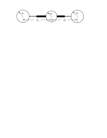
Figure 1: Schematics of the three-sphere swimmer. The two arms can open and close in a prescribed form, and this could lead to locomotion if the swimming strokes are nonreciprocal.

We begin with a simplified model geometry which consists of three spheres of radii $a_{i}$ ($i=1,2,3$) that are separated by two arms of lengths $L_{1}$ and $L_{2}$ as depicted in Fig. 1. Each sphere exerts a force $f_{i}$ on (and experiences a force $-f_{i}$ from) the fluid that we assume to be along the swimmer axis. In the limit $a_{i}/L_{j}\ll 1$, we can use the Oseen tensor lrnh ; Oseen to relate the forces and the velocities as

$$v_{1} = \frac{f_{1}}{6\pi\eta a_{1}}+\frac{f_{2}}{4\pi\eta L_{1}}+\frac{f_{3}}{4\pi\eta(L_{1}+L_{2})},$$ (1)

$$v_{2} = \frac{f_{1}}{4\pi\eta L_{1}}+\frac{f_{2}}{6\pi\eta a_{2}}+\frac{f_{3}}{4\pi\eta L_{2}},$$ (2)

$$v_{3} = \frac{f_{1}}{4\pi\eta(L_{1}+L_{2})}+\frac{f_{2}}{4\pi\eta L_{2}}+\frac{f_{3}}{6\pi\eta a_{3}}.$$ (3)

Note that in this simple one dimensional case, the tensorial structure of the hydrodynamic Green’s function (Oseen tensor) does not enter the calculations as all the forces and velocities are parallel to each other and to the position vectors. The swimming velocity of the whole object is the mean translational velocity, namely

$$V=\frac{1}{3}(v_{1}+v_{2}+v_{3}).$$ (4)

We are seeking to study autonomous net swimming, which requires the whole system to be force-free (i.e. there are no external forces acting on the spheres). This means that the above equations are subject to the constraint

$$f_{1}+f_{2}+f_{3}=0.$$ (5)

Eliminating $f_{2}$ using Eq. (5), we can calculate the swimming velocity from Eqs. (1), (2), (3), and (4) as

$$V_{0} = \frac{1}{3}\left[\left(\frac{1}{a_{1}}-\frac{1}{a_{2}}\right)+\frac{3}{2}\left(\frac{1}{L_{1}+L_{2}}-\frac{1}{L_{2}}\right)\right]\left(\frac{f_{1}}{6\pi\eta}\right)$$

$$+ \frac{1}{3}\left[\left(\frac{1}{a_{3}}-\frac{1}{a_{2}}\right)+\frac{3}{2}\left(\frac{1}{L_{1}+L_{2}}-\frac{1}{L_{1}}\right)\right]\left(\frac{f_{3}}{6\pi\eta}\right),$$

where the subscript $0$ denotes the force-free condition. To close the system of equations, we should either prescribe the forces (stresses) acting across each linker, or alternatively the opening and closing motion of each arm as a function of time. We choose to prescribe the motion of the arms connecting the three spheres, and assume that the velocities

$${\dot{L}}_{1} = v_{2}-v_{1},$$ (7)

$${\dot{L}}_{2} = v_{3}-v_{2},$$ (8)

are known functions. We then use Eqs. (1), (2), (3), and (5) to solve for $f_{1}$ and $f_{3}$ as a function of ${\dot{L}}_{1}$ and ${\dot{L}}_{2}$. Putting the resulting expressions for $f_{1}$ and $f_{3}$ back in Eq. (LABEL:V-f1-f3), and keeping only terms in the leading order in $a_{i}/L_{j}$ consistent with our original scheme, we find the average swimming velocity to the leading order.

III Swimming Velocity

The result of the above calculations is the lengthy expression of Eq. (46) reported in Appendix A. This result is suitable for numerical studies of swimming cycles with arbitrarily large deformations. For the simple case where all the spheres have the same radii, namely $a=a_{1}=a_{2}=a_{3}$, Eq. (LABEL:V-f1-f3) simplifies to

$$V_{0}=\frac{a}{6}\left[\left(\frac{{\dot{L}}_{2}-{\dot{L}}_{1}}{L_{1}+L_{2}}\right)+2\left(\frac{{\dot{L}}_{1}}{L_{2}}-\frac{{\dot{L}}_{2}}{L_{1}}\right)\right],$$ (9)

plus terms that average to zero over a full swimming cycle. Equation 9 is also valid for arbitrarily large deformations.

We can also consider relatively small deformations and perform an expansion of the swimming velocity to the leading order. Using

$$L_{1} = \ell_{1}+u_{1},$$ (10)

$$L_{2} = \ell_{2}+u_{2},$$ (11)

in Eq. (46), and expanding to the leading order in $u_{i}/\ell_{j}$, we find the average swimming velocity as

$$\overline{V_{0}}=\frac{K}{2}\;\overline{(u_{1}\dot{u}_{2}-\dot{u}_{1}u_{2})},$$ (12)

where

$$K=\frac{3\;a_{1}a_{2}a_{3}}{(a_{1}+a_{2}+a_{3})^{2}}\left[\frac{1}{\ell_{1}^{2}}+\frac{1}{\ell_{2}^{2}}-\frac{1}{(\ell_{1}+\ell_{2})^{2}}\right].$$ (13)

In the above result, the averaging is performed by time integration in a full cycle. Note that terms proportional to $u_{1}\dot{u}_{1}$, $u_{2}\dot{u}_{2}$, and $u_{1}\dot{u}_{2}+\dot{u}_{1}u_{2}$ are eliminated because they are full time derivatives and they average out to zero in a cycle. Equation (12) clearly shows that the average swimming velocity is proportional to the enclosed area that is swept in a full cycle in the configuration space [i.e. in the $(u_{1},u_{2})$ space]. This result, which is valid within the perturbation theory, is inherently related to the geometrical structure of theory the low Reynolds number swimming studied by Shapere and Wilczek geometry . Naturally, the swimmer can achieve higher velocities if it can maximize this area by introducing sufficient phase difference between the two deformation cycles (see below). We also note that the above result is more general than what was previously considered in Ref. 3SS , which corresponded to the class of configurational changes that happen one at a time, i.e. spanning rectangular areas in the configuration space note .

We can actually obtain Eq. (12) from a rather general argument. Since the deformation of the arms is prescribed, the instantaneous net displacement velocity of the swimmer should take on a series expansion form of $v(t)=A_{i}{\dot{u}}_{i}+B_{ij}{\dot{u}}_{i}{u}_{j}+C_{ijk}{\dot{u}}_{i}{u}_{j}{u}_{k}+\cdots,$ where the coefficients $A_{i}$, $B_{ij}$, $C_{ijk}$, etc. are purely geometrical prefactors (i.e. involving only the length scales $a_{i}$’s and $\ell_{i}$’s). Terms of higher order than one in velocity will have to be excluded on the grounds that in Stokes hydrodynamics forces are linearly dependent on (prescribed) velocities, and then the velocity any where else is also linearly proportional to the forces, which renders an overall linear dependency of the swimming velocity on set velocities. Moreover, higher order terms in velocity would require a time scale such as the period of the motion to balance the dimensions, which is not a quantity that is known to the system at any instant (i.e. would require nonlocal effects). Since the motion is periodic and we should average over one complete cycle to find the net swimming velocity, we can note that the only combination that survives the averaging process up to the second order is $u_{1}\dot{u}_{2}-\dot{u}_{1}u_{2}$, which yields Eq. (12). Note that this argument works even if the spheres have finite large radii that are not small comparable to the average length of the arms.

It is instructive at this point to examine a few explicit examples of swimming cycles for the three-sphere swimmer.

III.1 Harmonic Deformations

Let us consider harmonic deformations for the two arms, with identical frequencies $\omega$ and a mismatch in phases, namely

$$u_{1}(t)=d_{1}\cos(\omega t+\varphi_{1}),$$ (14)

$$u_{2}(t)=d_{2}\cos(\omega t+\varphi_{2}).$$ (15)

The average swimming velocity from Eq. (12) reads

$$\overline{V_{0}}=\frac{K}{2}\;d_{1}d_{2}\omega\sin(\varphi_{1}-\varphi_{2}).$$ (16)

This result shows that the maximum velocity is obtained when the phase difference is $\pi/2$, which supports the picture of maximizing the area covered by the trajectory of the swimming cycle in the parameter space of the deformations. A phase difference of $0$ or $\pi$, for example, will create closed trajectories with zero area, or just lines.

III.2 Simultaneous Switching and Asymmetric Relaxation

Thinking about practical aspects of implementing such swimming strokes in real systems, it might appear difficult to incorporate a phase difference in the motion of the two parts of a swimmer. In particular, for small scale swimmers we would not have direct mechanical access to the different parts of the system and the deformations would be more easily triggered externally by some kind of generic interaction with the system, such as shining laser pulses. In this case, we need to incorporate a net phase difference in the response of the two parts of the system to simultaneous triggers. This can be achieved if the two parts of the system have different relaxation times. To illustrate this, imagine that the arms of the swimmer could switch their lengths via exponential relaxation between two values of $\ell_{i}-d_{i}/2$ and $\ell_{i}+d_{i}/2$ back and forth as a switch is turned on and off. The deformation can be written as

$$u_{i}(t)=\left\{\begin{array}[]{ll}d_{i}\left[-\frac{1}{2}+\frac{1-e^{-t/\tau_{i}}}{1-e^{-T/2\tau_{i}}}\right],&\;0<t<\frac{T}{2},\\ \\ d_{i}\left[-\frac{1}{2}+\frac{e^{-t/\tau_{i}}-e^{-T/\tau_{i}}}{e^{-T/2\tau_{i}}-e^{-T/\tau_{i}}}\right],&\;\frac{T}{2}<t<T,\end{array}\right.$$ (17)

for $i=1,2$, where $\tau_{i}$’s are the corresponding relaxation times, and $T$ is the (common) period of the switchings. We find

$$\overline{V_{0}}=\frac{K}{8}\;d_{1}d_{2}\left(\frac{1}{\tau_{1}}-\frac{1}{\tau_{2}}\right)\;{\cal F}\left(\frac{T}{4\tau_{1}},\frac{T}{4\tau_{2}}\right),$$ (18)

where

$${\cal F}(x,y)=\frac{1}{\sinh x\;\sinh y}\left[\frac{\sinh(x+y)}{(x+y)}-\frac{\sinh(x-y)}{(x-y)}\right].$$ (19)

The above function is a smooth and monotonically decaying function of both $x$ and $y$ that is always positive, and it has the asymptotic limits ${\cal F}(0,0)=\frac{2}{3}$, ${\cal F}(x,y\to\infty)=0$, and ${\cal F}(x\to\infty,y)=0$. Here, the phase mismatch is materialized in the difference in the relaxation times, despite the fact that the deformations are switched on and off simultaneously.

III.3 Noisy Deformations

Another important issue in practical situations is the inevitability of random or stochastic behavior of the deformations. In small scales, Brownian agitations of the environment become a significant issue, and we would like to know how feasible it is to extract a net coordinated swimming motion from a set of two noisy deformation patterns. Using the Fourier transform of the deformations ($i=1,2$)

$$u_{i}(t)=\int\frac{d\omega}{2\pi}\;u_{i}(\omega)e^{i\omega t},$$ (20)

we can calculate the time-averaged swimming velocity of Eq. (12) as

$$\overline{V_{0}}=\frac{K}{2}\;\frac{1}{T}\int\frac{d\omega}{2\pi}\;i\omega\overline{\left[u_{2}(\omega)u_{1}(-\omega)-u_{1}(\omega)u_{2}(-\omega)\right]}.$$ (21)

For deformations that have discrete spectra ($i=1,2$), namely

$$u_{i}(t)=\sum_{n}\;d_{in}\cos(\omega_{n}t+\varphi_{in}),$$ (22)

we find

$$\overline{V_{0}}=\frac{K}{2}\sum_{n}\;\overline{d_{1n}d_{2n}\omega_{n}\sin(\varphi_{1n}-\varphi_{2n})}.$$ (23)

This shows that a net swimming is the result of coordinated motions of the different modes in the frequency spectrum, and the net velocity is the sum of the individual contributions of the different modes. As long as we can achieve a certain degree of coherence in a number of selected frequencies, we can have a net swimming despite the noisy nature of the deformations.

IV Internal Forces and Stresses

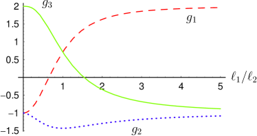
Figure 2: (color online.) The dimensionless forces exerted on the fluid at the locations of the spheres [defined in Eq. (30)] as functions of the relative size of the two arms. Dashed line (red) corresponds to Sphere 1, dotted line (blue) corresponds to Sphere 2, and solid line (green) corresponds to Sphere 3.

The interaction of the spheres and the medium involves forces as these parts of the swimmer make their ways through the viscous fluid when performing the swimming strokes. We have calculated these forces for a general swimmer, but since their expressions are quite lengthy, we choose to present them only in the particular case where all the spheres have equal radii, namely $a_{1}=a_{2}=a_{3}=a$. For arbitrarily large deformations, we find

$$f_{1} = \frac{\pi\eta a^{2}}{2}\left[4\;\frac{{\dot{L}}_{1}}{L_{2}}+2\;\frac{{\dot{L}}_{2}}{L_{1}}+\frac{{\dot{L}}_{1}-{\dot{L}}_{2}}{L_{1}+L_{2}}\right],$$ (24)

$$f_{2} = \frac{\pi\eta a^{2}}{2}\left[-2\;\frac{{\dot{L}}_{1}}{L_{2}}+2\;\frac{{\dot{L}}_{2}}{L_{1}}-2\;\frac{{\dot{L}}_{1}-{\dot{L}}_{2}}{L_{1}+L_{2}}\right],$$ (25)

$$f_{3} = \frac{\pi\eta a^{2}}{2}\left[-2\;\frac{{\dot{L}}_{1}}{L_{2}}-4\;\frac{{\dot{L}}_{2}}{L_{1}}+\frac{{\dot{L}}_{1}-{\dot{L}}_{2}}{L_{1}+L_{2}}\right],$$ (26)

up to terms that average to zero over a full cycle. One can check that the above expressions manifestly add up to zero, as they should. For small relative deformations, we find the following expressions for the average forces exerted on the fluid

$$\overline{f_{1}} = \frac{\pi\eta a^{2}}{2}\left[-\frac{1}{\ell_{1}^{2}}+\frac{2}{\ell_{2}^{2}}+\frac{1}{(\ell_{1}+\ell_{2})^{2}}\right]\overline{(u_{1}\dot{u}_{2}-\dot{u}_{1}u_{2})},$$

$$\overline{f_{2}} = \frac{\pi\eta a^{2}}{2}\left[-\frac{1}{\ell_{1}^{2}}-\frac{1}{\ell_{2}^{2}}-\frac{2}{(\ell_{1}+\ell_{2})^{2}}\right]\overline{(u_{1}\dot{u}_{2}-\dot{u}_{1}u_{2})},$$

$$\overline{f_{3}} = \frac{\pi\eta a^{2}}{2}\left[\frac{2}{\ell_{1}^{2}}-\frac{1}{\ell_{2}^{2}}+\frac{1}{(\ell_{1}+\ell_{2})^{2}}\right]\overline{(u_{1}\dot{u}_{2}-\dot{u}_{1}u_{2})}.$$

These forces are all proportional to the net average swimming velocity, with proportionality constants that depend on $\ell_{1}$ and $\ell_{2}$. Therefore, we can write a generic form

$$\overline{f_{i}}=\frac{3\pi\eta a}{2}\;\overline{V_{0}}\;g_{i},$$ (30)

for the forces in terms of the dimensionless factors $g_{i}$. These dimensionless forces are plotted in Fig. 2 as functions of the ratio between the lengths of the two arms, which is a measure of the asymmetry in the structure of the swimmer.

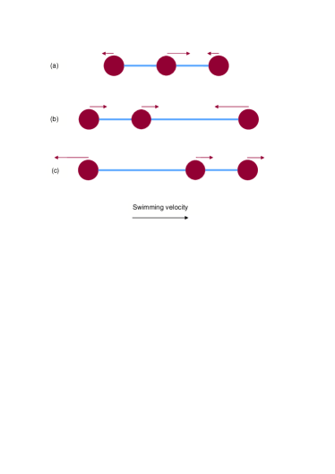
Figure 3: (color online.) The distribution of the average forces (denoted by arrows) exerted on the different spheres depending on the relative size of the arms. Case (a) corresponds to $\ell_{1}=\ell_{2}$, case (b) corresponds to $\ell_{1}\ll\ell_{2}$, and case (c) corresponds to $\ell_{1}\gg\ell_{2}$. The middle sphere always experiences a force that pushes it in the direction of swimming irrespective of the structure of the swimmer. Note that the above different cases do not correspond to the instantaneous forces exerted on each sphere during the swimming cycle.

It is instructive to examine the limiting behaviors of the forces as a function of the asymmetry. For $\ell_{1}\ll\ell_{2}$ we have $g_{1}=-1$, $g_{2}=-1$, and $g_{3}=2$ which means that the two closer spheres are in line with each other and the third sphere that is farther apart exerts the opposite force. The same trend is seen in the opposite limit $\ell_{1}\gg\ell_{2}$, where we have $g_{1}=2$, $g_{2}=-1$, and $g_{3}=-1$. In the symmetric case where $\ell_{1}=\ell_{2}$ we have $g_{1}=g_{3}=\frac{5}{7}$ and $g_{2}=-\frac{10}{7}$. Note that $g_{2}$ is always negative, which means that the middle sphere always experiences a force from the fluid that pushes it in the direction of swimming. The distribution of forces exerted on the spheres in these three different limits is shown schematically in Fig. 3.

It is interesting to note that in the symmetric case the forces are distributed so that their net dipole moment vanishes and the first non-vanishing moment of the forces becomes the quadrapole moment. This will cause the net fall-off of the velocity profile at large separations $r$ to change from $1/r^{2}$ (force dipoles) into $1/r^{3}$ (force quadrapoles). This behavior can be explained by a more general symmetry argument gareth .

V Force–Velocity Relation and Stall Force

The effect of an external force or load on the efficiency of the swimmer can be easily studied within the linear theory of Stokes hydrodynamics. When the swimmer is under the effect of an applied external force $F$, Eq. (5) should be changed as

$$f_{1}+f_{2}+f_{3}=F.$$ (31)

Following through the calculations of Sec. II above, we find that the following changes take place in Eqs. (1), (2), (3), and (4):

$$v_{1} \to v_{1}-\frac{F}{4\pi\eta L_{1}},$$ (32)

$$v_{2} \to v_{2}-\frac{F}{6\pi\eta a_{2}},$$ (33)

$$v_{3} \to v_{3}-\frac{F}{4\pi\eta L_{2}},$$ (34)

$$V \to V-\frac{1}{3}\left(\frac{1}{6\pi\eta a_{2}}+\frac{1}{4\pi\eta L_{1}}+\frac{1}{4\pi\eta L_{2}}\right)F.$$ (35)

These lead to the changes

$${\dot{L}}_{1} \to {\dot{L}}_{1}-\left(\frac{1}{6\pi\eta a_{2}}-\frac{1}{4\pi\eta L_{1}}\right)F,$$ (36)

$${\dot{L}}_{2} \to {\dot{L}}_{2}-\left(\frac{1}{4\pi\eta L_{2}}-\frac{1}{6\pi\eta a_{2}}\right)F,$$ (37)

in Eq. (46), which together with correction coming from Eq. (35) leads to the average swimming velocity

$$\overline{V}(F)=\overline{V_{0}}+\frac{F}{18\pi\eta a_{R}},$$ (39)

to the leading order, where $a_{R}$ is an effective (renormalized) hydrodynamic radius for the three-sphere swimmer. To the zeroth order, we have $a_{R}=\frac{1}{3}(a_{1}+a_{2}+a_{3})$ for the general case and there are a large number of correction terms at higher orders that we should keep in order to be consistent in our perturbation theory. Instead of reporting the lengthy expression for the general case, we provide the expression for $a_{1}=a_{2}=a_{3}=a$, which reads

$$\frac{1}{a_{R}} = \frac{1}{a}+\overline{\frac{1}{L_{1}}}+\overline{\frac{1}{L_{2}}}+\overline{\frac{1}{L_{1}+L_{2}}}$$ (40)

$$- \frac{a}{2}\overline{\left(\frac{1}{L_{1}}-\frac{1}{L_{2}}\right)^{2}}-\frac{a}{2}\overline{\frac{1}{(L_{1}+L_{2})^{2}}}.$$

We can also expand the deformation up to second order in $u_{i}$ and average the resulting expression. The result of this calculation is also lengthy and not particularly instructive, and is hence not reported here.

The force-velocity relation given in Eq. (39), which could have been expected based on linearity of hydrodynamics, yields a stall force

$$F_{s}=-18\pi\eta a_{R}\overline{V_{0}}.$$ (41)

Using the zeroth order expression for the hydrodynamic radius, one can see that this is equal to the Stokes force exerted on the three spheres moving with a velocity $\overline{V_{0}}$.

VI Power Consumption and Efficiency

Because we know the instantaneous values for the velocities and the forces, we can easily calculate the power consumption in the motion of the spheres through the viscous fluid. The rate of power consumption at any time is given as

$${\cal P}=f_{1}v_{1}+f_{2}v_{2}+f_{3}v_{3}=f_{1}(-{\dot{L}}_{1})+f_{3}({\dot{L}}_{2}),$$ (42)

where the second expression is the result of enforcing the force-free constrain of Eq. (5). Using the expressions for $f_{1}$ and $f_{3}$ as a function of ${\dot{L}}_{1}$ and ${\dot{L}}_{2}$, we find

$${\cal P} = 4\pi\eta a\left[1+\frac{a}{L_{1}}-\frac{1}{2}\frac{a}{L_{2}}+\frac{a}{L_{1}+L_{2}}\right]{\dot{L}}_{1}^{2}$$

$$+ 4\pi\eta a\left[1-\frac{1}{2}\frac{a}{L_{1}}+\frac{a}{L_{2}}+\frac{a}{L_{1}+L_{2}}\right]{\dot{L}}_{2}^{2}$$

$$+ 4\pi\eta a\left[1-\frac{1}{2}\frac{a}{L_{1}}-\frac{1}{2}\frac{a}{L_{2}}+\frac{5}{2}\frac{a}{L_{1}+L_{2}}\right]{\dot{L}}_{1}{\dot{L}}_{2},$$

(43)

for $a_{1}=a_{2}=a_{3}=a$.

We can now define a Lighthill hydrodynamic efficiency as

$$\eta_{\rm L}\equiv\frac{18\pi\eta a_{R}\overline{V_{0}}^{2}}{\overline{\cal P}},$$ (44)

for which we find to the leading order

$$\eta_{\rm L} = \frac{9}{8}\frac{a_{R}}{a}\;\frac{K^{2}\;\overline{(u_{1}\dot{u}_{2}-\dot{u}_{1}u_{2})}^{2}}{C_{1}\;\overline{\dot{u}_{1}^{2}}+C_{2}\;\overline{\dot{u}_{2}^{2}}+C_{3}\;\overline{\dot{u}_{1}\dot{u}_{2}}},$$ (45)

where $C_{1}=1+\frac{a}{\ell_{1}}-\frac{1}{2}\frac{a}{\ell_{2}}+\frac{a}{\ell_{1}+\ell_{2}}$, $C_{2}=1-\frac{1}{2}\frac{a}{\ell_{1}}+\frac{a}{\ell_{2}}+\frac{a}{\ell_{1}+\ell_{2}}$, and $C_{3}=1-\frac{1}{2}\frac{a}{\ell_{1}}-\frac{1}{2}\frac{a}{\ell_{2}}+\frac{5}{2}\frac{a}{\ell_{1}+\ell_{2}}$. It is interesting to note that for harmonic deformations (with single frequency) Eq. (45) is independent of the frequency and scales like $a^{2}d^{2}/\ell^{4}$, which reflects the generally low hydrodynamic efficiency of low Reynolds number swimmers. In this case, it is possible to find an optimal value for the phase difference that maximizes the efficiency feld .

VII Concluding Remarks

We have considered the simple model of a low Reynolds number swimmer, which is composed of three spheres that are linked by two phantom arms with negligible hydrodynamic interaction. Assuming arbitrary prescribed motion of the two arms, we have analyzed the motion of the swimmer and provided explicit expressions for the swimming velocity and other physical characteristics of the motion.

The simplicity of the model allows us to study the properties of the swimmer in considerable details using analytical calculations. This is a great advantage, as it can allow us to easily consider complicated problems involving such swimmers and could hopefully lead to new insights in the field of low Reynolds number locomotion. An example of such studies has already been performed by Pooley et al. who considered the hydrodynamic interaction of two such swimmers and found a rich variety of behaviors as a function of relative positioning of the two swimmers and their phase coherence gareth . This can be further generalized into a multi-swimmer system, and the collective floc behavior of such systems can then be studied using a “realistic” model for self-propellers at low Reynolds number that is faithful to the rules of the game. Knowing something about the internal structure of a swimmer will also allow us to study the synchronization problem more systematically sync .

Appendix A Swimming Velocity for Arbitrary Deformations

For the general case of a three-sphere swimmer based on the schematics in Fig. 1, we obtain the average swimming velocity to the leading order as

$$V_{0} = \frac{(a_{1}-a_{2})(a_{2}+a_{3})}{3a_{2}(a_{1}+a_{2}+a_{3})}\left[1+\frac{3}{2}\left(\frac{a_{1}a_{2}}{a_{2}-a_{1}}\right)\left(\frac{1}{L_{1}+L_{2}}-\frac{1}{L_{2}}\right)-3\left(\frac{a_{2}a_{3}}{a_{2}+a_{3}}\right)\frac{1}{L_{2}}\right.$$ (46)

$$\hskip 85.35826pt\left.+\frac{3}{a_{1}+a_{2}+a_{3}}\left(\frac{a_{2}a_{3}}{L_{2}}+\frac{a_{1}a_{2}}{L_{1}}+\frac{a_{3}a_{1}}{L_{1}+L_{2}}\right)\right]{\dot{L}}_{1}$$

$$+ \frac{a_{3}(a_{1}-a_{2})}{3a_{2}(a_{1}+a_{2}+a_{3})}\left[1+\frac{3}{2}\left(\frac{a_{1}a_{2}}{a_{2}-a_{1}}\right)\left(\frac{1}{L_{1}+L_{2}}-\frac{1}{L_{2}}\right)-\frac{3}{2}\left(\frac{a_{2}}{L_{1}}+\frac{a_{2}}{L_{2}}-\frac{a_{2}}{L_{1}+L_{2}}\right)\right.$$

$$\hskip 85.35826pt\left.+\frac{3}{a_{1}+a_{2}+a_{3}}\left(\frac{a_{2}a_{3}}{L_{2}}+\frac{a_{1}a_{2}}{L_{1}}+\frac{a_{3}a_{1}}{L_{1}+L_{2}}\right)\right]{\dot{L}}_{2}$$

$$+ \frac{a_{1}(a_{2}-a_{3})}{3a_{2}(a_{1}+a_{2}+a_{3})}\left[1+\frac{3}{2}\left(\frac{a_{2}a_{3}}{a_{2}-a_{3}}\right)\left(\frac{1}{L_{1}+L_{2}}-\frac{1}{L_{1}}\right)-\frac{3}{2}\left(\frac{a_{2}}{L_{1}}+\frac{a_{2}}{L_{2}}-\frac{a_{2}}{L_{1}+L_{2}}\right)\right.$$

$$\hskip 85.35826pt\left.+\frac{3}{a_{1}+a_{2}+a_{3}}\left(\frac{a_{2}a_{3}}{L_{2}}+\frac{a_{1}a_{2}}{L_{1}}+\frac{a_{3}a_{1}}{L_{1}+L_{2}}\right)\right]{\dot{L}}_{1}$$

$$+ \frac{(a_{2}-a_{3})(a_{1}+a_{2})}{3a_{2}(a_{1}+a_{2}+a_{3})}\left[1+\frac{3}{2}\left(\frac{a_{2}a_{3}}{a_{2}-a_{3}}\right)\left(\frac{1}{L_{1}+L_{2}}-\frac{1}{L_{1}}\right)-3\left(\frac{a_{1}a_{2}}{a_{1}+a_{2}}\right)\frac{1}{L_{1}}\right.$$

$$\hskip 85.35826pt\left.+\frac{3}{a_{1}+a_{2}+a_{3}}\left(\frac{a_{2}a_{3}}{L_{2}}+\frac{a_{1}a_{2}}{L_{1}}+\frac{a_{3}a_{1}}{L_{1}+L_{2}}\right)\right]{\dot{L}}_{2}.$$

This expression can be used in numerical studies of the swimming motion for arbitrarily large deformations and geometric characteristics.

References

- (1) G.I. Taylor, Proc. Roy. Soc. London A 209, 447-461 (1951).
- (2) E.M. Purcell, American Journal of Physics 45, 3-11 (1977).
- (3) A. Najafi and R. Golestanian, Phys. Rev. E 69, 062901 (2004).
- (4) J.E. Avron, O. Kenneth, O. Gat, Phys. Rev. Lett. 93, 186001 (2004); J.E. Avron, O. Kenneth, and D.H. Oaknin, New J. Phys. 7 234 (2005).
- (5) R. Dreyfus, J. Baudry and H.A. Stone, Eur. Phys. J. B 47, 161 (2005).
- (6) I.M. Kulic, R. Thaokar and H. Schiessel, Europhys. Lett. 72, 527 (2005).
- (7) A. Lee, H.Y. Lee, and M. Kardar, Phys. Rev. Lett. 95, 138101 (2005).
- (8) A. Najafi and R. Golestanian, J. Phys.: Condens. Matter 17, S1203 (2005).
- (9) B.U. Felderhof, Phys. Fluids 18, 063101 (2006).
- (10) E. Gauger and H. Stark, Phys. Rev. E 74, 021907 (2006).
- (11) A.M. Leshansky, Phys. Rev. E 74, 012901 (2006).
- (12) D. Tam and A.E. Hosoi, Phys. Rev. Lett. 98, 068105 (2007).
- (13) D.J. Earl, C.M. Pooley, J.F. Ryder, I. Bredberg and J.M. Yeomans, J. Chem. Phys. 126 064703 (2007).
- (14) C.M. Pooley, G.P. Alexander, and J.M. Yeomans, Phys. Rev. Lett. 99, 228103 (2007).
- (15) C.M. Pooley and A.C. Balazs, Phys. Rev. E 76, 016308 (2007).
- (16) E. Lauga, Phys. Rev. E 75, 041916 (2007).
- (17) K. Kruse et al., unpublished.
- (18) R. Dreyfus, J. Baudry, M.L. Roper, M. Fermigier, H.A. Stone, J. Bibette, Nature 437, 862 (2005).
- (19) W.F. Paxton et al., J. Am. Chem. Soc. 126, 13424 (2004); S. Fournier-Bidoz et al., Chem. Comm., 441-443 (2005); N. Mano and A. Heller, J. Am. Chem. Soc. 127, 11574 (2005); R. Golestanian, T.B. Liverpool, and A. Ajdari, Phys. Rev. Lett. 94, 220801 (2005); New J. Phys. 9, 126 (2007); G. Rückner and R. Kapral, Phys. Rev. Lett. 98, 150603 (2007); J.R. Howse et al., Phys. Rev. Lett. 99, 048102 (2007).
- (20) L.E. Becker, S.A. Koehler, and H.A. Stone, J. Fluid Mech. 490, 15 (2003).
- (21) R. Golestanian, Eur. Phys. J. E, in press (2008); [arXiv:0711.3772].
- (22) R. Golestanian and A. Ajdari, Phys. Rev. Lett. 100, 038101 (2008).
- (23) J. Happel and H. Brenner, Low Reynolds Number Hydrodynamics, (Prentice-Hall, Englewood Cliffs, New Jersey, 1965).
- (24) C.W. Oseen, Neuere Methoden und Ergebnisse in der Hydrodynamik (Akademishe Verlagsgesellschaft, Leipzig, 1927).
- (25) We would like to point out that in Ref. 3SS a relation is proposed for the average swimming velocity which numerically fits best to a large portion of the parameters encompassing small and large deformations, rather than attempting to systematically perform a perturbative calculation. This is also discussed in Ref. earl .
- (26) A. Shapere and F. Wilczek, Phys. Rev. Lett. 58, 2051 (1987)
- (27) M.J. Kim and T.R. Powers, Phys. Rev. E 69, 061910 (2004); M. Reicherta and H. Stark, Eur. Phys. J. E 17, 493 (2005); A. Vilfan and F. Jülicher, Phys. Rev. Lett. 96, 058102 (2006).