Scaling Law for Radius of Gyration and Its Dependence on Hydrophobicity

Abstract

Scaling law for geometrical and dynamical quantities of biological molecules is an interesting topic. According to Flory’s theory, a power law between radius of gyration and the length of homopolymer chain is found, with exponent 3/5 for good solvent and 1/3 for poor solvent. For protein in physiological condition, a solvent condition in between, a power law with exponent $\sim 2/5$ is obtained. In this paper, we present a unified formula to cover all above cases. It shows that the scaling exponents are generally correlated with fractal dimension of a chain under certain solvent condition. While applying our formula to protein, the fractal dimension is found to depend on its hydrophobicity. By turning a physical process-varying hydrophobicity of a chain by amino acid mutation, to an equivalent chemical process-varying polarity of solvent by adding polar or nonpolar molecules, we successfully deprive this relation, with reasonable agreement to statistical data. And it will be helpful for protein structure prediction. Our results indicate that the protein may share the same basic principle with homopolymer, despite its specificity as a heteropolymer.

I Introduction

It is well known that a protein can refold to its native structure from denatured state under physiology condition. However, the mechanism underlying is still unknown and becomes one of basic intellectual challenges in molecular biology1 . In the study of protein folding, radius of gyration, defined as $R_{g}=\sqrt{\frac{1}{N}\sum_{i=1}^{N}(\vec{R}_{i}-<\vec{R}>)^{2}},\;<\vec{R}>=\frac{1}{N}\sum_{i=1}^{N}\vec{R}_{i}$, is introduced as an important quantity. It is not only able to describe the static compactness of a protein structure, but also the folding process from denatured state to native state. Experimentally, Takahashi et. al. used small-angle X-ray scattering method to measure time evolution of $R_{g}$ during a protein’s folding process. In their study, significant changes in radius of gyration from unfolded to folded conformations were observed in several proteins by pH jump2 .

An interesting question is about the relationship between $R_{g}$ and other physical quantities. In this paper, we present a scaling law between radius of gyration and the length of protein chain ($N$) by exploiting Protein Data Bank: $R_{g}\propto N^{\nu}$, which has also been reported by other authors8 ; 9 ; 10 ; 11 ; 12 . Through generalizing former Flory’s theory3 , we get a new unified formula, which can be applied to polymer in poor solvent, polymer in good solvent and protein under physiological condition etc. It shows that the scaling exponents are generally correlated with the fractal dimension of a chain. We also study the influence of hydrophobicity on compactness of a protein chain. By considering the equivalence between protein-solvent coupled systems, we turn a physical process-varying hydrophobicity of a chain by amino acid mutation, to a chemical process-varying polarity of solvent by adding polar or nonpolar molecules. This enables us to derive a relation between hydrophobicity and fractal dimension, with good agreement to statistical data.

The paper is organized as follows: In Section II, a scaling law of radius of gyration for proteins under physiological condition is presented. In section III, we deprive our new unified formula based on Flory’s original theory. In Section IV, the influence of hydrophobicity on fractal dimension is studied. Section V will be a brief conclusion. In Appendix, the relation between scaling exponent and hydrophobicity is studied directly, in the same way as Section IV.

II Scaling exponent for protein under physiological condition

If neglect minor differences between amino acids, protein can be treated as a homopolymer. According to well-known Flory’s theory3 ; 4 ; 5 ; 6 , there exists a universal scaling law between radius of gyration and the length of polymer chain.

$$R_{g}\propto N^{\nu},$$ (1)

where exponent $\nu$ depends on solvent condition. Under good solvent condition, monomers are separated by solvent molecules. Thus we have $\nu=3/5$. Under poor solvent condition, the chain is highly compressed by solvent pressure. And $\nu=1/3$ is as high as crystals.

However, proteins under physiological condition have their specificity. On one hand, they are compact due to hydrophobic interactions. On the other hand, they are usually not well-packed and contain many cavities inside7 . Geometrically, these cavities are a consequence of regular secondary structures in folded proteins. Furthermore, they are essential for biological functions, since they can serve as binding sites when contacting to other molecules. Therefore, folded proteins should be more compact than polymers in good solvent, and looser than highly compressed polymers in poor solvent, i.e., $1/3\leq\nu\leq 3/5$. This argument is confirmed by statistical study of over 37,000 protein structures from Protein Data Bank (PDB), which yields $\nu\approx 2/5$ (Fig.1) and agrees with the research of Arteca8 ; 9 ; 10 . It indicates that proteins in native state are not so compact as crystals, which is a bit different from current popular view11 .

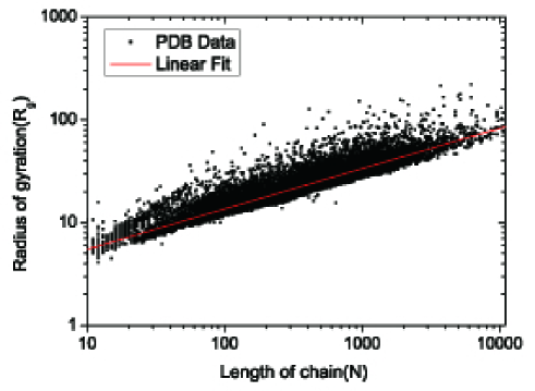
Figure 1: A log-log plot of 37162 protein structures in PDB, with $\nu=0.3916\pm 0.0008$ by least-quare linear fit.

The influence of secondary structure is also studied. In Fig. 2, we show statistical data for all-$\alpha$, all-$\beta$, $\alpha/\beta$ mixed protein structures (the fractions of amino acids in secondary structures are larger than $50\%$) and unstructured proteins (the fraction of amino acids in secondary structures is less than $20\%$) in PDB. Despite their great differences in secondary structure, their scaling exponent $\nu$ are all approximate to $2/5$. This result seems a bit contradictive to our common sense at first glance. Since it is easily to see that for single straight $\alpha$-helix, $\nu=1$; for perfect planar $\beta$-sheet, $\nu=1/2$. They are both largely apart from $\nu=2/5$. However, as secondary structure is a local characteristic, while scaling exponent $\nu$ mainly depends on over-all topological properties. When the protein is large enough to contain sufficient secondary structures, their influence will be quite limited. These results imply that there may exist a unified mechanism for the scaling law between radius of gyration and the length of protein chain.

(a)

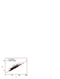
(b)

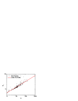
(c)

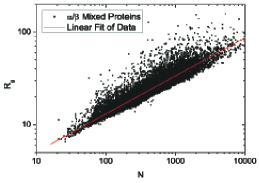
(d)

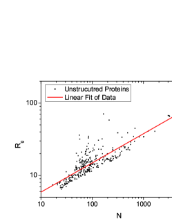
Figure 2: Log-log plot of proteins with different secondary structure. (a) 3080 all-$\alpha$ proteins with $N_{\alpha}/N\geq 0.5$ ($N_{\alpha}$ is the number of amino acids in $\alpha$-helix. And single $\alpha$-helix is excluded.). $\nu=0.4026\pm 0.0036$ by least-quare linear fit. (b) 334 all-$\beta$ proteins with $N_{\beta}/N\geq 0.5$ ($N_{\beta}$ is the number of amino acids in $\beta$-sheet). $\nu=0.3838\pm 0.00746$. (c) 25804 $\alpha/\beta$ mixed proteins with $(N_{\alpha}+N_{\beta})/N\geq 0.5$. $\nu=0.4166\pm 0.0010$. (d) 839 unstructured proteins with $(N_{\alpha}+N_{\beta})/N\leq 0.2$. $\nu=0.4038\pm 0.0097$.

III Generalized Flory’s Theory

To obtain a unified formula for scaling law valid under different solvent conditions, we try to generalize Flory’s original theory3 ; 4 ; 5 ; 6 . We assume that the chain is made up of N monomers, which are indistinguishable from each other. Then its overall size is mainly determined by two following effects: excluded volume effect that tends to swell the chain, and elastic interaction that tends to shrink the chain.

Firstly, the excluded volume effect is a consequence of repulsive interactions between monomers, with energy (two-body repulsive interaction) given by3 ; 4 ; 5 ; 6

$$E_{\mathrm{rep}}=k_{B}Tv\frac{N^{2}}{R_{g}^{3}},$$ (2)

where $v$ is single monomer’s volume.

Then, we calculate the elastic energy. Generally speaking, this term is originated from contact interactions between monomers, which include hydrophobic interaction between monomers and solvent molecules, covalent bonds, hydrogen bonds and Van der Waal’s interaction between neighboring monomers, etc. Since we are unable to give an explicit formula, we adopt harmonic approximation to find the dominant part.

Let $d_{ij}$ be the real distance between monomers $i$ and $j$. Then monomer $i$ is considered to be in contact with monomer $j$, if $d_{ij}\leq\delta$, where $\delta>0$ is some given constant. Let $d_{0}$ be average distance between any two contact monomers $i$ and $j$. $d_{0}$ is independent to index $i$ and $j$, and corresponds to the minimum of potential energy. Under harmonic approximation, the elastic energy of a chain with $N$ monomers is given by

$$E_{\mathrm{ela}}=\frac{1}{2}\sum_{i,j=1}^{N}\frac{1}{2}\kappa(d_{ij}-d_{0})^{2}\chi(d_{ij}),$$

$$\chi(d_{ij})=\left\{\begin{array}[]{ll}1,&\textrm{if $i\neq j$ and $d_{ij}\leq\delta$}\\ 0,&\textrm{else}\\ \end{array}\right.$$ (5)

where the first factor $1/2$ dues to double counting of monomers. And $\kappa$ is Hooke coefficient. Define root-mean-square contact distance ($d$) as

$$d^{2}=\frac{1}{\overline{n}}\sum_{j=1}^{N}d_{ij}^{2}\chi(d_{ij}),$$

where $\overline{n}=\sum_{j=1}^{N}\chi(d_{ij})$ is local contact number. $\overline{n}$ and $d$ are supposed to be independent to index $i$, for all monomers are equal in our treatment. On the other hand, we have

$$\sum_{j=1}^{N}d_{ij}\chi(d_{ij})=\overline{n}d_{0}.$$

So now we can rewrite $E_{ela}$ as

$$E_{\mathrm{ela}}=\frac{1}{4}\sum_{i=1}^{N}\kappa\overline{n}(d^{2}-d_{0}^{2})=\frac{1}{4}\overline{n}N\kappa d^{2}-\frac{1}{4}\overline{n}N\kappa d_{0}^{2},$$

As the second term is independent of $R_{g}$, it will be omitted in later discussions. Thus, we get

$$E_{\mathrm{ela}}=\frac{1}{4}\kappa\bar{n}Nd^{2}$$ (6)

In general, the root-mean-square contact distance $d$ is a function of $R_{g}$ and $N$ ($d=d(R_{g},N)$), and depends on compactness of a chain.

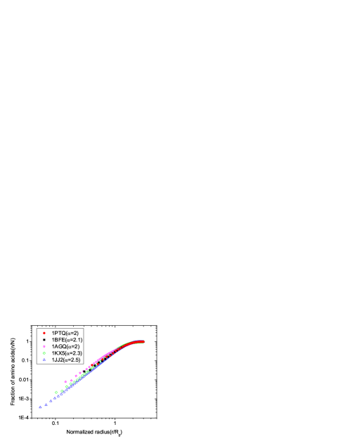
Figure 3: A log-log plot for 5 illustrative proteins, which are selected randomly from PDB except appropriate chain length. ($N=50,R_{g}=9.7$ for 1PTQ; $N=110,R_{g}=13.13$ for 1BFE; $N=373,R_{g}=26.98$ for 1AGQ; $N=1268,R_{g}=38.74$ for 1KX5; $N=6577,R_{g}=71.68$ for 1JJ2.) The data are obtained by counting the number of amino acids ($n$) within different given radius ($r$) starting at the geometrical center. It is clear that there exists a wide self-similarity region between small-scale and large-scale structure, with exponent $\alpha\approx 2$. Beyond this region, $\alpha$ drops to $1$ quickly, due to finite chain length.

As suggested by many authors, the protein can be regarded as a fractal in some extent12 ; 13 ; 14 ; 15 ; 16 ; 17 . If there exists a self-similarity in number density between small-scale and large-scale structure (Fig. 3), we can write

$$(\bar{n}+1)/d^{\alpha}=N/R_{g}^{\alpha}$$ (7)

where $\alpha$ stands for fractal dimension of a protein’s structure. Thus the root-mean-square contact distance is obtained as

$$d=(\bar{n}+1)^{1/\alpha}R_{g}/N^{1/\alpha}$$ (8)

Put into Eqn.(4),

$$E_{\mathrm{ela}}=\frac{1}{4}\kappa\bar{n}(\bar{n}+1)^{2/\alpha}\dfrac{R_{g}^{2}}{N^{2/\alpha-1}}$$ (9)

Hence, the total energy is given by

$$E=E_{\mathrm{rep}}+E_{\mathrm{ela}}=k_{B}Tv\frac{N^{2}}{R_{g}^{3}}+\frac{1}{4}\kappa\bar{n}(\bar{n}+1)^{2/\alpha}\dfrac{R_{g}^{2}}{N^{2/\alpha-1}}$$ (10)

In above argument, we neglect many other effects3 ; 4 ; 5 ; 6 , such as entropy effect ($E_{entropy}=\gamma R_{g}^{2}/N\propto N^{2\nu-1}$) and three-body repulsive interaction ($E_{three}=\mu N^{3}/R_{g}^{6}\propto N^{3-6\nu}$) etc. Nevertheless, in the region we are interested ($\nu\in(\frac{1}{3},\frac{3}{5})$, $\alpha\in(1,3)$), it is easily to check that $\lim_{N\rightarrow\infty}E_{entropy}/E_{ela}=0,\;\lim_{N\rightarrow\infty}E_{three}/E_{rep}=0$.

In equilibrium state, radius of gyration can be estimated by minimizing the total energy $E$. Let $\partial E/\partial R_{g}=0$, we have

$$R_{g}=\left[\frac{6k_{B}Tv}{\kappa\bar{n}(\bar{n}+1)^{2/\alpha}}\right]^{1/5}N^{\frac{\alpha+2}{5\alpha}}\propto N^{\frac{\alpha+2}{5\alpha}}$$ (11)

which gives

$$\nu=\dfrac{\alpha+2}{5\alpha}$$ (12)

In Fig.4, we can see that classical Flory’s theory acts as an extreme case in our new formula. In good solvent, polymer becomes loose, and can be modeled as a one-dimensional long chain. Thus $\alpha=1$, which gives $\nu=3/5$. In poor solvent, polymer is highly compressed by solvent pressure, and becomes as well-packed as crystals. It means $\alpha=3$, then $\nu=1/3$.

In the case of protein under physiological condition, we have $\alpha\approx 2$ (Fig.3), so $\nu\approx 2/5$. It suggests that many amino acid residues($\propto N$) are distributed at the surface of a protein; and the interior is not so compact as what having been thought before. This result is also supported by other researches7 ; 12 ; 13 ; 14 ; 15 ; 16 ; 17 .

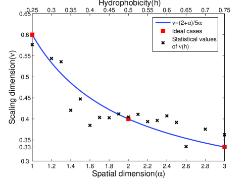
Figure 4: The blue solid curve is for Eqn.(9). The red squares are for three ideal cases respectively: polymer in good solvent ($\alpha=1$), protein under physiological condition ($\alpha=2$) and polymer in poor solvent ($\alpha=3$). The crosses stand for statistical values of exponent $\nu$ for proteins with different hydrophobicity ($h$). $\nu(h)$ is estimated by least-square linear fitting of uniformly selected statistical data (proteins with same hydrophobicity within $\pm 0.005$) from PDB. Data for $h<0.25$ and $h>0.75$, as well as $h=0.275,0.675,0.725$ are missing due to inadequate samples.

IV Dependence on Hydrophobicity

Above deduction is based on assumption of homopolymer. However, in fact, protein is a heteropolymer made up of twenty different kinds of amino acids. Thus exponent $\nu$ generally depends on the component of the chain, especially its hydrophobicity. To study this effect, a simple H-P model is introduced. Here we adopt the category method of Kyte and Doolittle18 . All amino acids with positive values in K-D method are regarded as hydrophobic (I, V, L, F, C, M, A, G); while other ones with negative values are regarded as hydrophilic (T, S, W, Y, P, H, E, N, Q, D, K, R).

The fraction of hydrophobic amino acids in a protein is defined as its hydrophobicity($h$). Then if all amino acids are hydrophilic ($h=0$), which just corresponds to good solvent condition, the protein will be fully extended with dimension $\alpha=1$. In this case, constrains arising from covalent bonds are dominant interaction against swelling tendency. If all amino acids are hydrophobic ($h=1$), corresponding to poor solvent condition, the protein is highly compressed by solvent pressure and dimension $\alpha=3$. Strong hydrophobic interactions are balanced by excluded volume effect between amino acid residues.

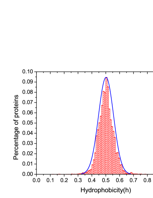
Figure 5: Hydrophobicity distribution of 33901 protein structures in PDB. Data is fitted by a Gaussian curve $Y=0.094\cdot e^{\frac{-(X-0.5)^{2}}{2*0.054^{2}}}$.

For natural proteins, their hydrophobicity has a Gaussian-like distribution (Fig.5). In the region $h\in[0.4,0.6]$, scaling exponent is almost unchanged (Fig.4), $\nu\approx 2/5$. For $h<0.4$ or $h>0.6$, the number of natural proteins are quite limited. And their corresponding exponent $\nu$ varies largely. Especially for $h<0.25$ or $h>0.75$, the proteins can regarded as total hydrophilic or hydrophobic respectively. These results hint appropriate hydrophobicity is essential to maintain overall structure of a natural protein.

To study how hydrophobicity affects scaling exponnet, we try to theoretically predict $\alpha=\alpha(h),\;h\in[0,1]$.

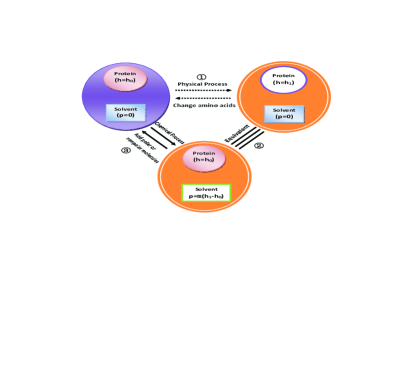
Figure 6: Illustration for our main idea of studying $\alpha(h)$. Process ①-③ correspond to Eqn.(10)-(12) separately. Process ① is what we want to study. However, varying the hydrophobicity of a protein by amino acid mutation is not a chemical process, and hard to grasp. Process ② is our main assumption: varying the hydrophobicity of a protein is equivalent to varying the polarity of solvent. Process ③ is a real chemical reaction. By adding polar or nonpolar molecules, we can control the polarity of solvent.

We record the state of protein-solvent coupled system as $X${Hydrophobicity of Protein, Polarity of Solvent}$\equiv X\{h,p\}$. Then two proteins with different hydrophobicity in same water solution are written as

$$X\{h=h_{0},p=0\}\rightleftarrows X\{h=h_{1},p=0\}$$ (13)

Here the polarity of water solution is set to zero. If we know how above two states are changed into one another, we can predict the relation of $\alpha(h)$. However, above process is connected by amino acid mutation, which is not a chemical reaction and not easy to analyze. Here we adopt an alternative way, which is based on the assumption that varying the hydrophobicity of a protein is equivalent to varying the polarity of solvent. According to biochemistry, the hydrophobicity of a protein is closely related to the polarity of solvent. The more polar the solvent is, the more hydrophobic the protein is; while the less polar the solvent is, the more hydrophilic the protein will be. Thus we can assume following two systems are equivalent

$$X\{h=h_{1},p=0\}\equiv X\{h=h_{0},p=m(h_{1}-h_{0})\}$$ (14)

Here, we adopt a linear relationship between hydrophobicity and polarity, and its validity remains to be verified by experiments. From Eqn.(10) and (11), we can turn a physical process-varying hydrophobicity of a chain by amino acid mutation, to a chemical process-varying polarity of solvent by adding polar or nonpolar molecules (Fig.6). Thus, Eqn.(10) is equivalent to following process

$$X\{h=h_{0},p=0\}\rightleftharpoons X\{h=h_{0},p=m(h_{1}-h_{0})\}$$ (15)

Now the study on $\alpha(h)$ is changed into a chemical reaction. Suppose there are three separated stable thermal states $X_{1},X_{2},X_{3}$, which represent proteins in good solvent, under physiological condition and in poor solvent respectively. Their corresponding fractal dimensions are $\alpha(X_{1})=1$, $\alpha(X_{2})=2$ and $\alpha(X_{3})=3$.

We start from the state under physiological condition. When the condition is changed from water solution to good solvent, which can be done by adding nonpoler molecules ($N$), proteins will change from $X_{2}$ state to $X_{1}$ state, according to following chemical process

$$X_{2}\rightleftharpoons^{k_{1}}_{k_{-1}}X_{1}$$ (16)

Here reaction constants $k_{1}$ and $k_{-1}$ depend on the concentration of nonpolar molecules added ($[N]$ is normalized to be in $[0,1]$). Let $[X_{i}]$ be the fraction of proteins in state $X_{i}$. When system reach equilibrium state, we have

$$[X_{1}]/[X_{2}]=k_{1}/k_{-1}=K_{1}([N])$$ (17)

Here, a power function is chosen for above relation

$$K_{1}([N])=C_{1}[N]^{m_{1}}$$ (18)

Due to the conservation law of matter $[X_{1}]+[X_{2}]=1$, we have $[X_{1}]=K_{1}/(1+K_{1}),\;[X_{2}]=1/(1+K_{1})$. Then for proteins with solvent condition between water solution and good solvent, their average fractal dimension is given by a Hill function

$$\alpha=\alpha(X_{1})[X_{1}]+\alpha(X_{2})[X_{2}]=1+\frac{1}{1+C_{1}[N]^{m_{1}}}$$ (19)

with $[N]\in[0,1]$ and $C_{1}\gg 1$.

Similarly, we can study proteins changed from $X_{2}$ state to $X_{3}$ state, or from water solution to poor solvent, which can be done by adding poler molecules ($P$). This process is described as

$$X_{2}\rightleftharpoons^{k_{2}}_{k_{-2}}X_{3}$$ (20)

Thus in the equilibrium state,

$$[X_{3}]/[X_{2}]=k_{2}/k_{-2}=K_{2}([P])=C_{2}[P]^{m_{2}}$$ (21)

$[P]$ is the concentration of polar molecules added, and normalized to be in $[0,1]$. As $[X_{2}]+[X_{3}]=1$, $[X_{2}]=1/(1+K_{2}),\;[X_{3}]=K_{2}/(1+K_{2})$. For proteins with solvent condition from water solution to poor solvent, the average fractal dimension is given by

$$\alpha=\alpha(X_{2})[X_{2}]+\alpha(X_{3})[X_{3}]=3-\frac{1}{1+C_{2}[P]^{m_{2}}}$$ (22)

with $[P]\in[0,1]$ and $C_{2}\gg 1$.

Take a linear relationship between hydrophobicity and polarity: $h=\frac{1-[N]}{2}$ and $h=\frac{1+[P]}{2}$, we can fit the statistical data by Eqn.(16) and (19) with appropriate values of $m_{1},\;m_{2},\;C_{1},\;C_{2}$ (Fig.7).

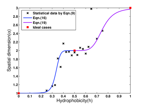
Figure 7: Statistical data for $\alpha=\alpha(h)$, which is obtained through inverse transform of data shown in Fig.4 by Eqn.(9). Fitting curve are given by Eqn.(16) and (19), with $m_{1}=8,\;m_{2}=5,\;C_{1}=3^{8},\;C_{2}=2^{5}$.

A suggested function of $\alpha=\alpha(h)$ is given by

$$\alpha(h)=\left\{\begin{array}[]{ll}1+\frac{1}{1+3^{8}(1-2h)^{8}},&\textrm{for h$\in$[0,0.5]}\\ 3-\frac{1}{1+2^{5}(2h-1)^{5}},&\textrm{for h$\in$(0.5,1]}\\ \end{array}\right.$$ (25)

V Conclusion

In summary, we have derived a unified formula for the scaling law between radius of gyration and the length of homopolymer chain. It shows that this exponent is generally correlated with the fractal dimension of a chain under certain solvent condition. Our new formula covers the well-known Flory’s theory for polymers under good and poor solvent conditions as two extreme cases. It can be applied to proteins under physiological condition ($\nu\approx 2/5$) too, with a predicted fractal dimensional $\alpha\approx 2$. Influence of hydrophobicity on the compactness of a protein has also been studied through a simple H-P model. By considering the equivalence between protein-solvent coupled systems, we turn a physical process-varying the hydrophobicity of a chain by amino acid mutation, to a chemical process-varying the polarity of solvent by adding polar or nonpolar molecules. This enables us to derive a functional relation between hydrophobicity and fractal dimension, with reasonable agreement to statistical data. This relation will be helpful for protein structure prediction. Our results indicate that the protein may share the same basic principle with homopolymer, despite its speciality as a heteropolymer. Hope this work can shed light on the mechanism of protein folding and stability of protein structures.

Appendix A Direct study of $\nu(h)$

Although we can get $\nu(h)$ according to Eqn.(9) and (20), a direct prediction is also possible in the same way as Sec.III. Suppose $\nu(X_{1})=3/5,\nu(X_{2})=2/5,\nu(X_{3})=1/3$, the average scaling exponent is given by

$$\nu=\nu(X_{1})[X_{1}]+\nu(X_{2})[X_{2}]$$

$$\quad=\frac{3}{5}-\frac{1}{5(1+C_{1}[N]^{m_{1}})}$$

$$\quad=\frac{3}{5}-\frac{1}{5[1+C_{1}(1-2h)^{m_{1}}]}$$ (26)

for $h\in[0,0.5]$, $C_{1}\gg 1$; and

$$\nu=\nu(X_{2})[X_{2}]+\nu(X_{3})[X_{3}]$$

$$\quad=\frac{1}{3}+\frac{1}{15(1+C_{2}[P]^{m_{2}})}$$

$$\quad=\frac{1}{3}+\frac{1}{15[1+C_{2}(2h-1)^{m_{2}}]}$$ (27)

for $h\in(0.5,1]$, $C_{2}\gg 1$.

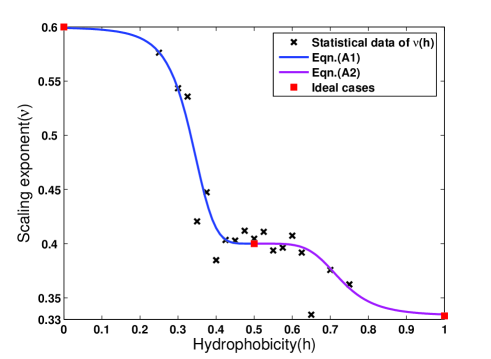
Figure 8: The statistical data is the same as Fig.4. Fitting curves are given by Eqn.(A1) and (A2), with $m_{1}=m_{2}=5,\;C_{1}=3^{5},\;C_{2}=2.2^{5}$.

A suggested function of $\nu=\nu(h)$ is given by

$$\nu(h)=\left\{\begin{array}[]{ll}\frac{3}{5}-\frac{1}{5[1+3^{5}(2h-1)^{5}]},&\textrm{for h$\in$[0,0.5]}\\ \frac{1}{3}+\frac{1}{15[1+2.2^{5}(2h-1)^{5}]},&\textrm{for h$\in$(0.5,1]}\\ \end{array}\right.$$ (30)

References

- (1) C. Branden, J. Tooze, Introduction to protein structure, 2nd edition, Garland Publishing (1998).
- (2) S. Akiyama, S. Takahashi, T. Kumura, K. Ishimori, I. Morishima, Y. Nishikawa, T. Fujisawa, PNAS, 99, 1329-1334 (2002). T. Uzawa, S. Akiyama, T. Kimura, S. Takahashi, K. Ishimori, I. Morishima, T. Fujisawa, PNAS, 101, 1171-1176 (2004). T. Kimura, T. Uzawa, K. Ishimori, I. Morishima, S. Takahashi, T. Konno, S. Akiyama, T. Fujisawa, PNAS, 102, 2748-2753 (2005).
- (3) P.J. Flory, Principles of polymer chemistry, Cornell University Press (1953).
- (4) M. Doi and S.F. Edwards, The theroy of polymer dynamics, Clarendon Press, Oxford (1986).
- (5) A.Y. Grosberg and A.R. Khokhlov, Statistical Physics of Macromolecules, AIP Press (1994).
- (6) M. Rubinstein and R.H. Colby, Polymer Physics, Oxford University Press, 2003.
- (7) Jie Liang and K.A. Dill, Biophysical Journal, 81, 751-766 (2001).
- (8) G.A. Arteca, Physical Review E, 49, 2417-2428 (1994).
- (9) G.A. Arteca, Physical Review E, 51, 2600-2610 (1995).
- (10) G.A. Arteca, Physical Review E, 54, 3044-3047 (1996).
- (11) S. Takahashi and T. Fujishawa, The Second International Symposium on Frontiers of Applied Mathematics (2006).
- (12) D. Stauffer and A. Aharony, Introduction to percolation theory, Taylor & Francis (1985).
- (13) T.G. Dewey and M.M. Datta, Biophysical Journal, 56, 415-420 (1989).
- (14) J.F. Huang and C.Q. Liu, Journal of Biomathematics, 12, 385-392 (1997).
- (15) M.B. Enright and D.M. Leitner, Physical Review E, 71, 011912 (2005).
- (16) M.A. Moret, J.G.V. Miranda, E. Nogueira Jr., M.C. Santana and G.F. Zebende, Physical Review E, 71, 012901 (2005).
- (17) M.A. Moret, M.C. Santana, E. Nogueira Jr. and G.F. Zebende, Physica A, 361, 250-254 (2006).
- (18) J. Kyte and R.A. Doolittle, J.Mol.Biol, 157, 105-132 (1982).