Static and dynamic structure factors
in three-dimensional randomly diluted Ising models

Abstract

We consider the three-dimensional randomly diluted Ising model and study the critical behavior of the static and dynamic spin-spin correlation functions (static and dynamic structure factors) at the paramagnetic-ferromagnetic transition in the high-temperature phase. We consider a purely relaxational dynamics without conservation laws, the so-called model A. We present Monte Carlo simulations and perturbative field-theoretical calculations. While the critical behavior of the static structure factor is quite similar to that occurring in pure Ising systems, the dynamic structure factor shows a substantially different critical behavior. In particular, the dynamic correlation function shows a large-time decay rate which is momentum independent. This effect is not related to the presence of the Griffiths tail, which is expected to be irrelevant in the critical limit, but rather to the breaking of translational invariance, which occurs for any sample and which, at the critical point, is not recovered even after the disorder average.

I Introduction and Summary

The effect of disorder on magnetic systems remains, after decades of investigation, a not fully understood subject. It is then natural to investigate relatively simple models, to try to understand the common features of disordered systems. In this regard, randomly diluted spin systems are quite interesting. First, they represent simple models which describe the universal properties of the paramagnetic-ferromagnetic transition in uniaxial antiferromagnets with impurities Belanger-00 and, in general, the order-disorder transition in Ising systems in the presence of uncorrelated local dilution. Second, they give the opportunity for investigating general problems concerning the effects of disorder on the critical behavior. Indeed, several important results, theoretical developments, and approximation schemes found for these models have been later generalized to more complex systems like spin glasses, quantum disordered spin models, etc….

In this paper we consider three-dimensional randomly diluted Ising (RDI) systems. Their critical behavior has been extensively studied. Belanger-00 ; PV-02 ; FHY-03 There is now ample evidence that the magnetic transition in these systems, if it is continuous, belongs to a unique universality class, and several universal properties are now known quite accurately. Beside the static critical behavior, we also investigate the dynamic critical behavior, considering a purely relaxation dynamics without conservation laws, the so-called model A, HH-77 which is appropriate for uniaxial antiferromagnets. We focus on the dynamic (time-dependent) spin-spin correlation function

$$G(x_{2}-x_{1},t_{2}-t_{1})\equiv\overline{\langle\sigma(x_{1},t_{1})\,\sigma(x_{2},t_{2})\rangle},$$ (1)

where $\sigma(x,t)$ is an Ising variable, the overline indicates the quenched average over the disorder probability distribution, and $\langle\cdot\cdot\cdot\rangle$ indicates the thermal average. From the function $G(x,t)$, one obtains the static (equal-time) structure factor $\widetilde{G}(k)$ and the dynamic structure factor $\widehat{G}(k,\omega)$. They are physically relevant quantities, which can be measured in neutron or X-ray scattering experiments. footBorn It is therefore interesting to study the effects of disorder on these physical quantities, and check whether disorder gives rise to qualitative changes with respect to pure systems. We investigate their scaling behavior close to the magnetic transition for $T\to T_{c}^{+}$ in the high-temperature phase. As we shall see, while the critical behavior of the static structure factor is very similar to that in pure Ising systems, the critical behavior of the dynamic structure factor is significantly different; in particular, the large-momentum behavior shows some new features.

Since the critical region in the paramagnetic phase, i.e. for $T\gtrsim T_{c}$, is located in the Griffiths phase,Griffiths ; v-06 it is mandatory to discuss first the relevance of the so-called Griffiths singularities and Griffiths tails for the universal critical behavior of the correlation functions when $T\rightarrow T_{c}^{+}$. In fact, one of the most notable features of randomly diluted spin systems is the existence of the so-called Griffiths phase for $T_{c}<T<T_{p}$, where $T_{p}$ is the critical temperature of the pure system. This is essentially related to the fact that, in the presence of disorder, the critical temperature $T_{c}$ is lower than $T_{p}$, and therefore, in the temperature interval $T_{c}<T<T_{p}$, there is a nonvanishing probability to find compact clusters without vacancies (Griffiths islands) that are fully magnetized. They give rise to essential nonanalyticities in thermodynamic quantities.Griffiths ; v-06 Moreover, these clusters are responsible for a nonexponential tail in dynamic correlation functions.Bray-88 ; DRS-88 ; Bray-89 ; CMM-98 In the case of RDI systems one can show that

$$G(x,t)\approx G_{G}(t)=B\exp[-C(\ln t)^{3/2}],$$ (2)

for any finite $x$ and $t\to\infty$, which implies a diverging relaxation time. We should mention that these effects are quite difficult to detect, and there is still no consensus on their experimental evidence even in systems with correlated disorder, in which these effects are magnified (see, e.g., Ref. expG, ; v-06, and references therein).

Griffiths essential singularities give quantitatively negligible effects on thermodynamic quantities and on the static critical behavior. One can argue that also the Griffiths tail (2) is irrelevant in the critical limit: the nonexponential tail does not contribute to the critical scaling function associated with $G(x,t)$.Bray-88 This is essentially due to the fact that $B$ and $C$ that appear in Eq. (2) are expected to be smooth functions of the temperature, approaching finite constants as $T\to T_{c}$. Thus, in the critical limit, $t\to\infty$, $T\to T_{c}$ at fixed $t\xi^{-z}$, where $\xi\sim(T-T_{c})^{-\nu}$ is the diverging correlation length, the nonexponential contribution simply vanishes. To understand why, let us consider the simplified situation in which the contributions to the autocorrelation function $G(x,t)$ due to the Griffiths islands and to the critical modes just sum as

$$G(t)\approx G_{C}(t)+G_{G}(t)=a\xi^{b}\exp(-ct\xi^{-z})+B\exp(-C(\ln t)^{3/2}),$$ (3)

where we neglect all couplings between Griffiths and critical modes. Here, $G_{C}(t)$ is the critical contribution, while $G_{G}(t)$ is the nonexponential Griffiths tail, which dominates for $t\gg t^{*}$, where $t^{*}$ is the time at which the two terms have the same magnitude. In the critical limit we have $t^{*}\sim\xi^{z}(\ln\xi)^{3/2}$. Since the critical limit is taken at fixed $t/\xi^{z}$, the relevant quantity is $t^{*}/\xi^{z}$, which diverges as $(\ln\xi)^{3/2}$ approaching the phase transition. This means that, for any fixed value of $t/\xi^{z}$, the condition $t\ll t^{*}$ is always satisfied sufficiently close to the critical temperature $T_{c}$, i.e., the nonexponential tail is negligible.

In order to determine the scaling behavior of the spin-spin correlation function (1), we perform Monte Carlo (MC) simulations of a three-dimensional RDI model on a simple cubic lattice and perturbative field-theoretical (FT) calculations. In the following we briefly summarize our main results.

The high-temperature critical behavior of the static structure factor $\widetilde{G}(k)$ is substantially analogous to that of $\widetilde{G}(k)$ in pure Ising systems.MPV-02 We consider the universal scaling function $g(Q^{2})\equiv{\widetilde{G}(k)/\widetilde{G}(0)}$, where $Q^{2}\equiv k^{2}\xi^{2}$ and $\xi$ is the second-moment correlation length. We find that $g(Q^{2})$ is very well approximated by the Ornstein-Zernike form (Gaussian free-field propagator) $g(Q)_{OZ}=1/(1+Q^{2})$: deviations are less than 1% for $Q\lesssim 5$ and increase to 5% at $Q\approx 50$. At large momenta, for $Q\gtrsim 10$ say, the static structure factor follows the Fisher-Langer law;FL-68 in particular, $g(Q^{2})\approx 0.92/Q^{2-\eta}$ with $\eta\approx 0.036$ for $Q\gtrsim 30$.

At variance with the static case, the dynamic structure factor displays substantial differences with respect to the pure case, even though, as expected, the Griffiths tail turns out to be irrelevant in the critical limit. We consider the universal scaling function

$$\Gamma(Q^{2},S)\equiv\lim_{T\rightarrow T_{c}^{+}}{\widetilde{G}(k,t)\over\widetilde{G}(k,0)}$$ (4)

in the critical limit $t\to\infty$, $k\to 0$, and $T\to T_{c}^{+}$ at fixed $Q$ and $S$. Here $S\equiv t/\tau_{\rm int}$, where $\tau_{\rm int}$ is the zero-momentum integrated autocorrelation time. Perturbative field theory shows that $\Gamma(Q^{2},S)$ decays exponentially, as in the case of pure systems, and this is confirmed by the simulation results. In pure Ising systems CMPV-03-2 the large-$S$ decay rate of $\Gamma(Q^{2},S)$ depends on $Q$: the large-$S$ behavior is very similar to that of $\Gamma(Q^{2},S)$ in the noninteracting Gaussian model, i.e. $\Gamma(Q^{2},S)\sim\exp[-\kappa(Q^{2})S]$, where $\kappa(Q^{2})=(1+Q^{2})$. This behavior drastically changes in the presence of random impurities; in particular, the large-$S$ decay rate becomes independent of $Q$. MC simulations and FT perturbative calculations show that, for generic values of $Q$, $\Gamma(Q^{2},S)$ has two different behaviors as a function of $S$. For small values of $S$, it decreases rapidly, with a rate that increases as $Q$ increases, as it does in the pure system.CMPV-03-2 For large $S$ instead, $\Gamma(Q^{2},S)$, and therefore $\widetilde{G}(k,t)$, decreases with a momentum-independent rate. For large $Q$ and $S$ we find

$$\Gamma(Q^{2},S)\sim S^{a}Q^{-\zeta}e^{-\kappa S},$$ (5)

where $a$ and $\zeta$ are critical exponents, and $\kappa$ does not depend on $Q$. We present a physical argument which relates the different large-$S$ behavior compared to pure systems to the loss of translational invariance. Such a phenomenon is obvious for a given fixed sample, but at the critical point translational invariance is not even recovered after averaging over disorder, because of the absence of self-averaging. Note that this phenomenon is only related to disorder and thus, it is expected in all systems in which disorder is relevant.

In general, the perturbative calculations predict a scaling behavior of the form

$$\Gamma(Q^{2},S)\sim Q^{-\zeta}f_{\zeta}(S),$$ (6)

for large $Q$, where $f_{\zeta}(S)$ is a function of $S$ such that $f_{\zeta}(S)\sim S^{a}e^{-\kappa S}$ for $S\to\infty$. This behavior implies that $G(x,t)$ is always nonanalytic for $x=0$ and any $t$. Indeed, because of Eq. (6), the integral

$$\int d^{d}Q\,Q^{2n}\Gamma(Q^{2},S)g(Q^{2})\sim\int d^{d}k\,k^{2n}\widetilde{G}(k,t)$$ (7)

diverges for $n\geq n_{c}\equiv(\zeta+2-d-\eta)/2$ ($d$ is the spatial dimension). Since the moments of $\widetilde{G}(k,t)$ are directly related to the derivatives of $G(x,t)$ with respect to $x$ computed for $x=0$, the $n$-th derivative of $G(x,t)$ diverges for $n\geq n_{c}$; hence $G(x,t)$ is not analytic at $x=0$. This implies that the scaling function $F(Y^{2},S)$, defined as

$$G(x,t)=\xi^{-d+2-\eta}F(Y^{2},S),\qquad Y^{2}\equiv x^{2}/\xi^{2},$$ (8)

behaves as $F(Y^{2},S)=f_{0}(S)+f_{\lambda}(S)|Y|^{\lambda}+\cdots$, where $\lambda=\zeta+2-d-\eta$, for $Y^{2}\to 0$. MC simulations indicate that $\zeta\approx 2$ in three dimensions, which implies $\lambda\approx 1$. This phenomenon does not occur in pure systems, since in this case the decay rate $\kappa$ depends on $Q$ and guarantees the integrability of the integrand which appears in Eq. (7) for any $n$. Therefore, $F(Y^{2},S)$ has an analytic expansion around $Y^{2}=0$, i.e., $F(Y^{2},S)=f_{0}(S)+f_{2}(S)Y^{2}+\cdots$. This nonanalyticity should be a general property of random models in which disorder is relevant, and not specific of RDI systems.

Finally, it is worth mentioning that in the case of three-dimensional randomly dilute multicomponent spin models, such as the $XY$ and the Heisenberg model, the effects of disorder found in RDI models are expected to be suppressed in the critical limit $T\rightarrow T_{c}^{+}$, and should only appear as peculiar scaling corrections. footalpha Indeed, the asymptotic critical behavior of the correlation functions is expected to be the same as that in the corresponding pure model, because the pure fixed point is stable under random dilution (according to the Harris criterion,Harris-74 dilution is irrelevant if the specific-heat exponent $\alpha$ of the pure system is negative).

The paper is organized as follows. In Sec. II we introduce the model that we study. In Sec. III we discuss the static structure factor in the high-temperature phase. In Sec. III.1 we define the quantities that are computed in the MC simulation, in Sec. III.2 we present some perturbative calculations, while in Sec. III.3 we discuss the MC results. In Sec. IV we discuss the dynamic structure factor. Again, we first define the basic quantities (Sec. IV.1), then we present a one-loop perturbative calculation (Sec. IV.2), and finally we report the MC results (Sec. IV.3 and IV.4). In the appendices we report some details of the perturbative calculations.

II The model

We consider the randomly site-diluted Ising model with Hamiltonian

$${\cal H}_{\rho}=-\sum_{<xy>}\rho_{x}\,\rho_{y}\;\sigma_{x}\sigma_{y},$$ (9)

where the sum is extended over all pairs of nearest-neighbor sites of a simple cubic lattice, $\sigma_{x}=\pm 1$ are Ising spin variables, and $\rho_{x}$ are uncorrelated quenched random variables, which are equal to 1 with probability $p$ (the spin concentration) and 0 with probability $1-p$ (the impurity concentration). For $p_{s}<p<1$, where $p_{s}$ is the site-percolation point ($p_{s}=0.3116081(13)$ on a simple cubic lattice BFMMPR-99 ), the model has a continuous transition with a ferromagnetic low-temperature phase.

MC simulations of RDI systems have shown rather conclusively (see, e.g., Refs. Belanger-00, ; PV-02, ; FHY-03, ; BFMMPR-98, ; HPPV-07, ; HPV-07, ) that their continuous transitions belong to a single universality class. The RDI universality class has been extensively studied by using FT methods and MC simulations. At present, the most accurate estimates of the critical exponents are HPPV-07 $\nu=0.683(2)$ and $\eta=0.036(1)$, obtained by a finite-size analysis of MC data. These estimates are in good agreement with those obtained by using field theory. An analysis of the six-loop perturbative expansions in the three-dimensional massive zero-momentum scheme gives PV-00 $\nu=0.678(10)$ and $\eta=0.030(3)$. Note the good agreement between FT and MC results, in spite of the fact that the perturbative FT series for dilute systems are not Borel summable. BMMRY-87 ; McKane-94 ; AMR-00 Also the correction-to-scaling exponents have been determined quite accurately. For the leading exponent $\omega$, MC simulations give HPV-07 $\omega=0.29(2)$ (older simulations gave $\omega=0.33(3)$HPPV-07 and $\omega=0.37(6)$BFMMPR-98 ), while field theory predicts $\omega=0.25(10)$,PV-00 $\omega=0.32(6)$.PS-00 For the next-to-leading exponent $\omega_{2}$, an appropriate analysis of the FT expansions givesHPPV-07 $\omega_{2}=0.82(8)$, which is consistent with the MC results for improved models.CMPV-03 ; HPPV-07 Beside the critical exponents, also the equation of state,CPV-eqst some amplitude ratios, CPV-eqst ; CPV-cross ; BCBJ-04 the universal crossover functions between the pure and the RDI fixed point CPV-cross and between the Gaussian and the RDI fixed point,CPV-cross ; FHY-00 and the crossover exponent in the presence of a weak random magnetic fieldcpv-03 have been computed.

A full characterization of the types of disorder that lead to a transition in the RDI universality class is still lacking. For instance, RDI transitions also occur in systems that are not ferromagnetic: this is the case of the Edwards-Anderson model ($\pm J$ Ising model), which is frustrated for any amount of disorder. EA-75 Nonetheless, the paramagnetic-ferromagnetic transition line that starts at the pure Ising transition point and ends at the multicritical Nishimori point belongs to the RDI universality class.HPPV-07-2

Beside the static behavior, we also consider the critical behavior of a purely relaxation dynamics without conservation laws, the so-called model A, as appropriate for uniaxial magnets.HH-77 The critical behavior of the model-A dynamics for RDI systems has been recently studied numerically (for a critical review of the existing results, see Ref. HPV-07, ). It has been shown that the relaxational dynamics belongs to a single dynamic universality class, HPV-07 characterized by the dynamic critical exponent $z=2.35(2)$.

For Hamiltonian (9) an accurate study of the dependence of the size of the corrections to scaling on $p$ is reported in Ref. HPPV-07, . It turns out that the leading scaling corrections associated with $\omega=0.29(2)$ are suppressed for $p=p^{*}=0.800(5)$, in agreement with the findings of Refs. BFMMPR-98, ; CMPV-03, . For this reason we have performed our simulations at $p=0.8$.

III Static structure factor in the high-temperature phase

III.1 Definitions

We consider the static (equal-time) two-point correlation function $G(x)\equiv G(x,t=0)$. In the infinite-volume limit we define the second-moment correlation length $\xi$

$$\xi^{2}\equiv-{1\over\chi}\left.{\partial\widetilde{G}(k)\over\partial k^{2}}\right|_{k^{2}=0},$$ (10)

where $\widetilde{G}(k)$ is the Fourier transform of $G(x)$ and

$$\chi\equiv\sum_{x}G(x)=\widetilde{G}(0)$$ (11)

is the magnetic susceptibility. It is also possible to define an exponential correlation length $\xi_{\rm exp}$. Given the infinite-volume $G(x)$, we define

$$\xi_{\rm exp}\equiv-\lim_{|x|\to\infty}{|x|\over\ln G(x)}.$$ (12)

In the critical limit $\xi$ and $\xi_{\rm exp}$ diverge. If $t_{r}\equiv(T-T_{c})/T_{c}$ and $T_{c}$ is the critical temperature, for $|t_{r}|\to 0$ we have in the thermodynamic limit

$$\xi,\xi_{\rm exp}\sim|t_{r}|^{-\nu},$$ (13)

where $\nu$ is a universal critical exponent. In the same limit, correlation functions have a universal behavior. For instance, the infinite-volume $\widetilde{G}(k)/\chi$ becomes a universal function of the scaling variable

$$Q^{2}\equiv k^{2}\xi^{2},\qquad\qquad$$ (14)

i.e. we can write in the scaling limit $k\to 0$, $t_{r}\to 0$ at fixed $Q$

$${\chi^{-1}\widetilde{G}(k)}\approx g(Q^{2}),$$ (15)

where $g(x)$ is universal. Moreover, the ratio $\xi^{2}/\xi_{\rm exp}^{2}$ converges to a universal constant $S_{M}$ defined by

$$\xi^{2}/\xi_{\rm exp}^{2}\approx S_{M}.$$ (16)

For a Gaussian theory the spin-spin correlation function shows the Ornstein-Zernike (OZ) behavior

$$\widetilde{G}_{OZ}(k)={Z\over k^{2}+r}.$$ (17)

It follows $\chi=Z/r$, $\xi^{2}=1/r$, and

$$g_{OZ}(Q^{2})={1\over 1+Q^{2}}\;.$$ (18)

Moreover, $S_{M}=1$.

Fluctuations change this behavior. For small $Q^{2}$, $g(Q^{2})$ is analytic, so that we can write the expansion

$$g(Q^{2})^{-1}=1+Q^{2}+\sum_{n=2}c_{n}Q^{2n},$$ (19)

where the coefficients $c_{n}$ parametrize the deviations from the OZ behavior. For large $Q^{2}$, the structure factor behaves as

$$g(Q^{2})\approx{C_{1}\over Q^{2-\eta}}\left(1+{C_{2}\over Q^{(1-\alpha)/\nu}}+{C_{3}\over Q^{1/\nu}}+\cdots\right),$$ (20)

a behavior predicted theoretically by Fisher and Langer FL-68 and proved in the FT framework in Refs. BAZ-74, ; BLZ-74, .

III.2 Field-theory results

We determined the coefficients $c_{n}$ by using two different FT approaches: the $\sqrt{\epsilon}$-expansion approach, in which the renormalization-group parameters are computed as series in powers of $\sqrt{\epsilon}$, $\epsilon=4-d$, and the massive zero-momentum (MZM) approach, in which one works directly in three dimensions. We computed the first few coefficients $c_{n}$ to $O(\epsilon^{3/2})$ in the $\sqrt{\epsilon}$ expansion, and to four loops in the MZM scheme. The corresponding expansions are reported in App. A. Setting $\epsilon=1$ in the $\sqrt{\epsilon}$ expansions (87), we obtain $c_{2}=-4\times 10^{-4}$, $c_{3}=1.0\times 10^{-5}$, $c_{4}=-4\times 10^{-7}$, and $c_{5}=2\times 10^{-8}$. In the MZM approach, resumming the perturbative expansions (90) as discussed in Ref. PV-00, , we obtain

$$c_{2}=-4(1)\times 10^{-4},$$ (21)

$$c_{3}=1.2(3)\times 10^{-5},$$ (22)

$$c_{4}=-5(2)\times 10^{-7}.$$ (23)

These results are fully consistent with those obtained in the $\sqrt{\epsilon}$ expansion, in spite of the fact that in that case we have not applied any resummation and we have simply set $\epsilon=1$. We can also compute $S_{M}$. Since the coefficients $c_{n}$ are very small, we obtain

$$S_{M}\approx 1+c_{2}=0.9996(1),$$ (24)

where we used the estimate (21) of $c_{2}$. As in the Ising case,CPRV-98 ; MPV-02 the coefficients $c_{n}$ show the pattern

$$|c_{n}|\ll|c_{n-1}|\ll...\ll|c_{2}|\ll 1\qquad\qquad{\rm for}\qquad n\geq 3.$$ (25)

This is consistent with the expected analyticity properties of $\widetilde{G}(k)$. Since the complex-plane singularity in $\widetilde{G}(k)^{-1}$ that is closest to the origin is expected to be the three-particle cut located at $k=\pm 3i/\xi_{\rm exp}$,FS-75 ; Bray-76 the function $g(Q^{2})^{-1}$ is analytic up to $Q^{2}=-9S_{M}$. It follows that $c_{n}\approx-c_{n-1}/(3\sqrt{S_{M}})$, at least asymptotically.

The large-$Q$ behavior can be investigated in the $\sqrt{\epsilon}$ expansion. The three-loop calculation of the two-point function reported in App. A.1 allows us to determine the perturbative expansion of the coefficients $C_{i}$ appearing in Eq. (20). Setting $\epsilon=1$ in the expressions (89), we obtain $C_{1}\approx 0.95$, $C_{2}+C_{3}=-0.96$.

In order to compare with the experimental and numerical data it is important to determine $g(Q^{2})$ for all values of $Q$. For the pure Ising structure factor, several interpolations have been proposed with the correct large- and small-$Q$ behavior. FB-67 ; TF-75 ; FS-75 ; Bray-76 ; FB-79 ; BBC-82 ; MPV-02 The most successful one is due to Bray,Bray-76 which incorporates the expected singularity structure of $g(Q^{2})$. In this approach, one assumes $1/g(Q^{2})$ to be well-defined in the complex $Q^{2}$ plane, with a cut on the negative real $Q^{2}$ axis, starting at the three-particle cut $Q^{2}=-r^{2}$ with $r^{2}=9S_{M}$. Then, one obtains the spectral representation

$$H(Q^{2}) \equiv \int_{r}^{\infty}du\,u^{1-\eta}{F(u)\over Q^{2}+u^{2}},$$

$${1\over g(Q^{2})} = 1+{Q^{2}H(Q^{2})\over S_{M}H(-S_{M})},$$ (26)

where $F(u)$ is the spectral function, which must satisfy $F(+\infty)=1$, $F(u)=0$ for $u<r$, and $F(u)\geq 0$ for $u\geq r$.

In order to obtain an approximation one must specify $F(u)$. Bray Bray-76 proposed to use a spectral function that gives exactly the Fisher-Langer asymptotic behavior, i.e.

$$F_{B}(u)={P_{1}(u)-P_{2}(u)\cot{1\over 2}\pi\eta\over P_{1}(u)^{2}+P_{2}(u)^{2}},$$ (27)

where

$$P_{1}(u) = 1+{C_{2}\over u^{p}}\cos{\pi p\over 2}+{C_{3}\over u^{1/\nu}}\cos{\pi\over 2\nu},$$

$$P_{2}(u) = {C_{2}\over u^{p}}\sin{\pi p\over 2}+{C_{3}\over u^{1/\nu}}\sin{\pi\over 2\nu},$$ (28)

with $p\equiv(1-\alpha)/\nu$. To obtain a numerical expression we fix $\nu=0.683$, $\eta=0.036$,HPPV-07 and use the estimate (24) of $S_{M}$. We must also fix $C_{2}$ and $C_{3}$. Bray proposes to fix $C_{2}+C_{3}$ to its $\epsilon$-expansion value (in our case $C_{2}+C_{3}=-0.96$) and then to determine these constants by requiring $F_{B}(u=r)=0$. These conditions give $C_{2}=-8.04$ and $C_{3}=7.07$. As a check, we can compare the estimates of $c_{n}$ and $C_{1}$ obtained by using Bray’s approximation $g_{B}(Q^{2})$ with the previously quoted results. We obtain

$$C_{1}={2\sin\pi\eta/2\over\pi}S_{M}H(-S_{M})\approx 0.92,$$ (29)

and $c_{2}\approx-4\cdot 10^{-4}$, $c_{3}\approx 9\cdot 10^{-6}$, $c_{4}\approx-4\cdot 10^{-7}$. These results are in very good agreement with those obtained before.

III.3 Monte Carlo results

In this section we study Hamiltonian (9) at $p=0.8$ in the high-temperature phase, with the purpose of determining the infinite-volume spin-spin correlation function $\widetilde{G}(k)$. We perform simulations on lattices of size $32\leq L\leq 256$ in the range $0.275\leq\beta\leq 0.2856$ [note thatHPV-07 $\beta_{c}=0.2857431(3)$]. The number of samples varies with $N$, being of the order of 3000, 10000, 30000, 40000 for $L=256,128,64,32$. For each sample, we start from a random configuration, run 1000 Swendsen-Wang and 1000 Metropolis iterations for thermalization, and then perform 2000 Swendsen-Wang sweeps. At each iteration we measure the correlation function $G(x;\beta,L)$ and the structure factor $\widetilde{G}(k;\beta,L)$. Since rotational invariance is recovered in the critical limit, to speed up the Fourier transforms, we determine it as

$$\widetilde{G}(k;\beta,L)={1\over 3}\sum_{x,y,z}(e^{ikx}+e^{iky}+e^{ikz})\overline{\langle\sigma(0,0,0)\sigma(x,y,z)\rangle},$$ (30)

where the sum runs over the coordinates $(x,y,z)$ of the lattice sites. Of course, on a finite lattice $k$ can only assume the values $2\pi n/L$, where $n$ is an integer such that $0\leq n\leq L-1$. We also compute the second-moment correlation length $\xi(\beta,L)$ defined by

$$\xi(\beta,L)^{2}\equiv{\widetilde{G}(0;\beta,L)-\widetilde{G}(k_{\rm min};\beta,L)\over\hat{k}_{\rm min}^{2}\widetilde{G}(k_{\rm min};\beta,L)},$$ (31)

where $k_{\rm min}\equiv 2\pi/L$, $\hat{k}\equiv 2\sin k/2$. For $L\to\infty$, $\xi(\beta,L)$ converges to the infinite-volume definition (10) with $L^{-2}$ corrections.

In order to determine $g(Q^{2})$ we go through several different steps. First, for each $\beta$ and $L$ we interpolate the numerical data in order to obtain $\widetilde{G}(k;\beta,L)$ for any $k$ in the range $[0,\pi]$. For this purpose we fit the numerical results for $h(k;\beta,L)\equiv\widetilde{G}(0;\beta,L)/\widetilde{G}(k;\beta,L)$ to

$$h(k;\beta,L)=1+\sum_{n=1}^{n_{\rm max}}a_{n}\hat{k}^{2n},\qquad\hat{k}=2\sin{k\over 2}.$$ (32)

We increase $n_{\rm max}$ until the sum of the residuals ($\chi^{2}$) is less than half of the fitted points (those corresponding to $1\leq n\leq L-1$), i.e. $\chi^{2}<L/2$ (note that the data are strongly correlated and thus it makes no sense to require $\chi^{2}/{\rm DOF}\approx 1$, where ${\rm DOF}=L-1-n_{\rm max}$ is the number of degrees of freedom of the fit). In most of the cases we take $n_{\rm max}=5$, but in a few cases we had to take $n_{\rm max}$ as large as 10.

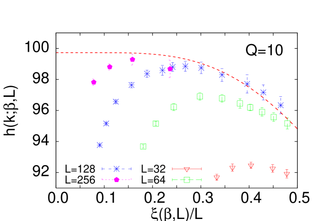
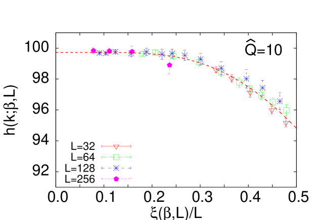
Figure 1: (Color online) Estimates of $h(k;\beta,L)$ vs $\xi(\beta,L)/L$ at fixed $Q=10$ (left) and $\widehat{Q}=10$ (right). We only report data corresponding to $k\leq k_{\rm max}=\pi/3$. We also report an interpolating curve (dashed line), which is obtained by fitting all data at fixed $\widehat{Q}$ reported on the right, as explained in the text.

Then, we investigate the finite-size effects. In the critical limit we expect

$$h(k;\beta,L)\approx F\left(Q\equiv k\xi(\beta,L),{\xi(\beta,L)\over L}\right).$$ (33)

Equivalently, one can also use

$$h(k;\beta,L)\approx F\left(\widehat{Q}\equiv\hat{k}\xi(\beta,L),{\xi(\beta,L)\over L}\right),$$ (34)

where $\hat{k}=2\sin k/2$. The two scaling forms are equivalent in the scaling limit $k\to 0$, $L\to\infty$, $\xi(\beta,L)\to\infty$ at fixed $Q$ (or $\widehat{Q}$) and $\xi(\beta,L)/L$; as a consequence, the function $F(x,y)$ is the same in the two cases. Indeed, $\hat{k}=k+O(k^{3})$, and thus, by keeping fixed $\widehat{Q}$ or $Q$, one only changes analytic corrections decaying as $L^{-2}$. In particular, whatever choice is made, the structure factor $g(Q^{2})$ is equal to $1/F(Q,0)$. Apparently, the corrections we are talking about here are less relevant than the nonanalytic corrections that should decay as $L^{-\omega_{2}}$, $\omega_{2}=0.82(8)$, and thus, a priori one would expect only small differences between the two approaches. Instead, as we show below, only by keeping $\widehat{Q}$ fixed is one able to determine the structure factor in the infinite-volume limit.

In Fig. 1 we show the numerical data for $Q=10$ (left) and $\widehat{Q}=10$ (right). On the left one observes very large size corrections which make impossible in practice the determination of the infinite-volume limit $\xi(\beta,L)/L\to 0$. On the right instead, there are no significant scaling corrections and all data fall approximately on a single curve. Size corrections are small for $\xi(\beta,L)/L\lesssim 0.20$ and the extrapolation to $\xi(\beta,L)/L\to 0$ is feasible. In the two panels we also show the interpolation of the data at fixed $\widehat{Q}$. As expected, the data at fixed $Q$ converge to this interpolation, but it is clear that no real information could have been obtained on the infinite-volume limit from the data in the left panel. In order to clarify why scaling at fixed $\widehat{Q}$ is so much better than scaling at fixed $Q$, we consider the lattice Gaussian model with nearest-neighbor couplings. In this case, the spin-spin correlation function on a finite lattice is given by

$$\widetilde{G}_{G}(k)={Z\over\hat{k}^{2}+r},$$ (35)

so that $\xi^{2}=1/r$ and

$$h(k)={1+\widehat{Q}^{2}}.$$ (36)

Thus, if we take the finite-size scaling limit at fixed $\widehat{Q}$ there are no finite-size corrections: the scaling is exact on any finite lattice. On the other hand, at fixed $Q$ we obtain

$$h(k)\approx(1+Q^{2})\left[1-{1\over 12L^{2}}{Q^{4}(L^{2}/\xi^{2})\over 1+Q^{2}}+\cdots\right].$$ (37)

In this case we have $1/L^{2}$ corrections, which diverge as $\xi/L\to 0$, exactly as we observe in our data. These corrections moreover increase with $Q$ and thus make it difficult, if not impossible, to estimate the structure factor.

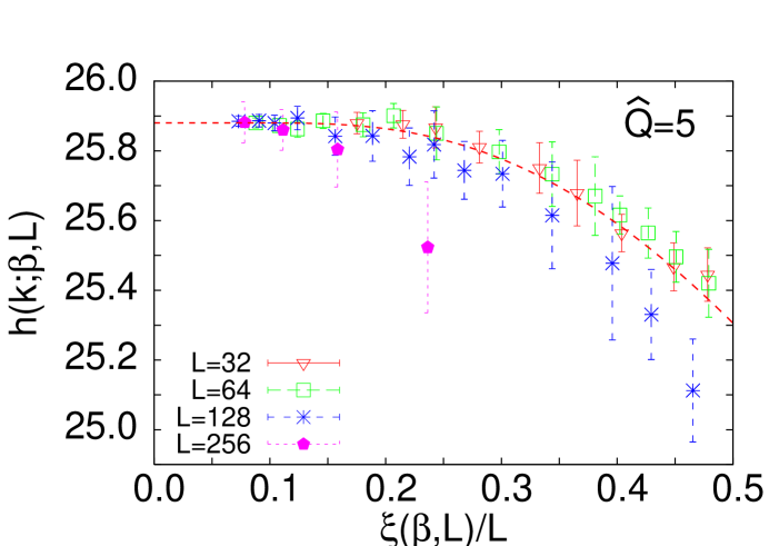
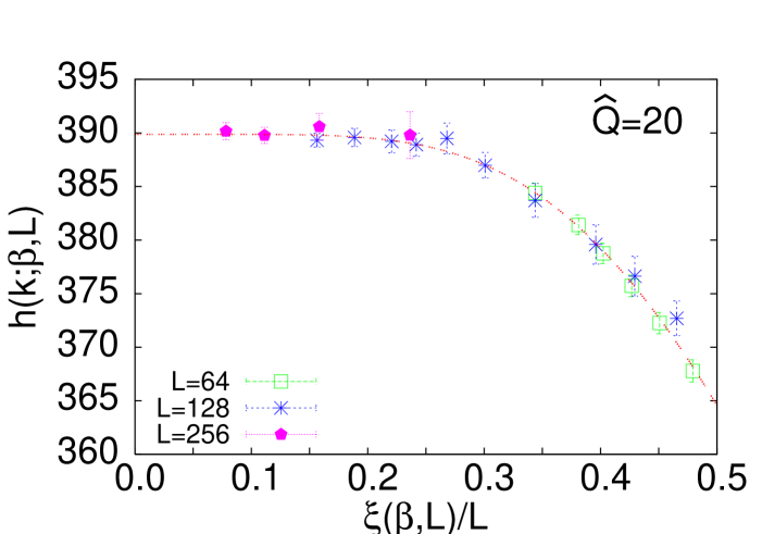
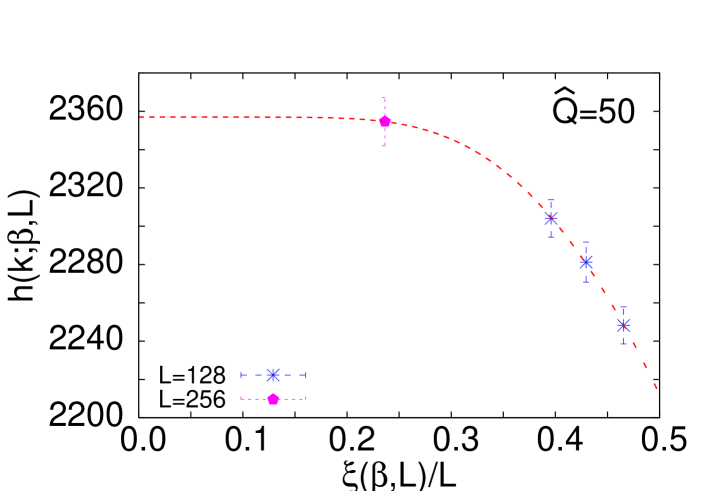
Figure 2: (Color online) MC results for $h(k;\beta,L)$ vs $\xi(\beta,L)/L$ at fixed $\widehat{Q}$ for three different values of $\widehat{Q}$: 5 (top), 20 (middle), 50 (bottom). Only data satisfying $k\leq k_{\rm max}=\pi/3$ are reported. The interpolation (dashed line) corresponds to a fit of the data with $L\geq 64$ as described in the text.

As a consequence of the above-reported discussion we consider below the finite-size scaling limit at fixed $\widehat{Q}$. In Fig. 2 we show $h(k;\beta,L)$ for $\widehat{Q}=5,20,50$. Since $\hat{k}$ can be at most 2, for each $\widehat{Q}$ we can only consider values of $\beta$ and $L$ such that $\xi(\beta,L)\geq\widehat{Q}/2$. However, since the critical limit is obtained for $k\to 0$, results close to the antiferromagnetic point $k=\pi$ cannot have a good scaling behavior. Therefore, in the analysis we have only considered values of $k$ such that $k\leq k_{\rm max}$. If $k_{\rm max}$ varies between $\pi/4$ and $\pi/3$, the final results are essentially independent of $k_{\rm max}$. The data reported in Figs. 1 and 2 scale as predicted by Eq. (34). Within the precision of our results some corrections to scaling are only visible for $\widehat{Q}=5$ and $\xi(\beta,L)/L\gtrsim 0.2$. They however die out fast in the interesting limit $\xi(\beta,L)/L\to 0$. Note also that, as $\widehat{Q}$ increases, the number of available points decreases and indeed we are not able to go beyond $\widehat{Q}\approx 50$ with our data.

In order to determine the infinite-volume limit $F(Q,0)$, we have taken all data satisfying $\xi(\beta,L)/L\leq 0.5$ and we have fitted them to

$$\left.h(k;\beta,L)\right|_{\hat{k}\xi=\widehat{Q}}=a_{0}+\sum_{j=1}^{j_{\rm max}}a_{j}\exp[-jL/\xi(\beta,L)].$$ (38)

The fitting form (38) is motivated by theory, which predicts exponentially small finite-size corrections in the high-temperature phase. With the precision of our data it is sufficient to take $j_{\rm max}=2$ to obtain $\chi^{2}/{\rm DOF}\lesssim 1$. The coefficient $a_{0}$ allows us to estimate $g(Q^{2})$: $g(Q^{2})=1/F(Q,0)=1/a_{0}$. The results for $k_{\rm max}=\pi/4$ and $\pi/3$ are essentially identical within errors up to $Q\approx 40$ (for $k_{\rm max}=\pi/4$ we do not have enough data to determine reliably $F(Q,0)$ for $Q\gtrsim 40$). In the following we take those corresponding to $k_{\rm max}=\pi/3$, which allow us to compute $g(Q^{2})$ up to $\widehat{Q}=50$. In order to detect scaling corrections we have repeated the analysis including each time only data such that $L\geq L_{\rm min}$. The results are essentially independent of $L_{\rm min}$. For instance, for $\widehat{Q}=5$, one of the values we considered in Fig. 2 (in this case some scaling corrections are present for $\xi(\beta,L)/L\gtrsim 0.20$), we obtain $a_{0}=25.881(6)$, 25.881(7), 25.882(9) for $L_{\rm min}=32,64,128$, respectively. This is due to the fact that $a_{0}$ is determined by the results at small values of $\xi(\beta,L)/L$ and in this range there are essentially no scaling corrections. In the following we choose conservatively $L_{\rm min}=64$.

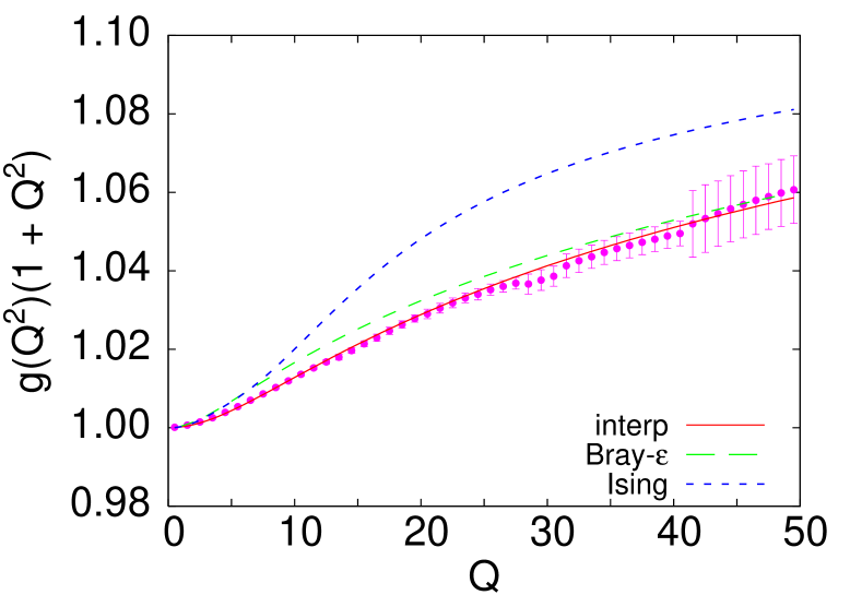
Figure 3: (Color online) Estimates of the scaling function $g(Q^{2})(1+Q^{2})$ for integer values of $Q$. We also report Bray’s approximation, in which $C_{2}+C_{3}$ is fixed to the $\sqrt{\epsilon}$ value (Bray-$\epsilon$), and the structure factor for the pure Ising model (Ising). The curve ”interp” (solid line) corresponds to the interpolation $g_{\rm int}(Q^{2})$ reported in Eq. (40).

Our final estimate of $g(Q^{2})$ is reported in Fig. 3. Deviations from the OZ behavior are quantitatively small and indeed at $Q=50$ the relative deviation is only 0.05. It is important to note that the estimates of $g(Q^{2})$ at different values of $Q$ are correlated since the estimates of $\widetilde{G}(k;\beta,L)$ for different values of $k$ are statistically correlated. This explains the regularity of the results. Note also that the error changes rather abruptly in a few cases. For instance, this occurs between $Q=40$ and $Q=41$. This happens because at $Q=40$, the estimate of $a_{0}$ is essentially determined by the result obtained for $\beta=0.2853$, $L=256$, which corresponds to $\xi(\beta,L)/L=0.158$ and $\hat{k}=0.989$. For $Q=41$ this lattice is no longer considered, since the corresponding $k$ exceeds $k_{\rm max}=\pi/3$ ($\hat{k}_{\rm max}=1$). For $Q=41$, the result with the smallest $\xi(\beta,L)/L$ corresponds to $\xi(\beta,L)/L=0.236$. The extrapolation to the infinite-volume limit is therefore much more imprecise.

For $Q\to\infty$, $g(Q^{2})\approx C_{1}/Q^{2-\eta}$, see Eq. (20). We fit the estimates of $\ln g(Q^{2})$ reported in Fig. 3 (they correspond to integer values of $Q$ between 1 and 50) to $a+(\eta-2)\ln Q$. If we include only data with $Q>Q_{\rm min}=15$ and 20, we obtain $\eta=0.032(1)$, 0.032(2), respectively. The error we quote here assumes that all data are independent, which is not the case. In order to determine the correct error bar, one should take into account the covariance among the results at different values of $Q$. This is not easy and therefore, in order to estimate the role of the statistical correlations, we use a more phenomenological approach. If $g_{\rm est}(Q^{2})$ is the estimate of $g(Q^{2})$ and $\sigma(Q^{2})$ the corresponding error, we consider new data $g_{\rm est}(Q^{2})-\sigma(Q^{2})$ with the same error and we repeat the fit. We obtain $\eta=0.029$ and $\eta=0.027$ for $Q_{\rm min}=15$ and 20. Analogously, if we consider $g_{\rm est}(Q^{2})+\sigma(Q^{2})$, we obtain $\eta=0.035,0.037$. This simple analysis indicates that $\pm 0.005$ is a plausible estimate of the statistical error. Therefore, we quote $\eta=0.032(5)$ as our final result. This estimate is in good agreement with that reported in Ref. HPPV-07, , $\eta=0.036(1)$, obtained from a finite-size scaling analysis of the susceptibility. In order to estimate $C_{1}$, we consider $g(Q^{2})Q^{2-\eta}$, fixing $\eta$ to $\eta=0.036(1)$. HPPV-07 For $Q\gtrsim 20$ this quantity is essentially constant: $g(Q^{2})Q^{2-\eta}=0.921(1)$, 0.920(1), 0.917(2), 0.919(3), for $Q=20,25,30,35$. We thus take

$$C_{1}=0.919(3)[3]$$ (39)

as our final estimate. The error in brackets gives the variation of the estimate as $\eta$ varies by one error bar ($\pm 0.001$). This estimate is close to the FT result $C_{1}\approx 0.95$ and in perfect agreement with the estimate (29) obtained by using Bray’s approximation for the spectral function, $C_{1}\approx 0.92$. Indeed, as can be seen in Fig. 3, Bray’s interpolation represents a very good approximation of the numerical data, deviations being quite tiny.

In Fig. 3 we also report the structure factor in pure Ising systems (we use the phenomenological approximation reported in Ref. MPV-02, , see their Eq. (30) with $Q_{\rm max}=15$ and $n_{\rm max}=6$). In the pure case, deviations from the OZ behavior are larger: the addition of impurities has the effect of reducing the deviations from the OZ behavior.

Finally, we report a phenomenological interpolation which reproduces well our numerical data and is consistent with the large $Q^{2}$ behavior, $g(Q^{2})\approx 0.919Q^{0.036}/(1+Q^{2})$:

$$g_{\rm int}(Q^{2})={(1+0.0227953Q^{2}+0.0000839355Q^{4})^{0.009}\over 1+Q^{2}}.$$ (40)

IV Dynamic structure factor in the high-temperature phase

In this section we consider the dynamic behavior of the Metropolis algorithm, which is a particular example of a relaxational dynamics without conservation laws, the so-called model A, as appropriate for magnetic systems. In Ref. HPV-07, we computed the dynamic critical exponent, obtaining $z=2.35(2)$. Here, we focus on the dynamic structure factor.

IV.1 Definitions

To investigate the dynamic behavior we consider the time-dependent two-point correlation function (1) and its Fourier transform $\widetilde{G}(k,t)$ with respect to the $x$ variable. Then, we define the integrated autocorrelation time

$$\tau_{\rm int}(k)\equiv{1\over 2}\sum_{t=-\infty}^{\infty}\,{\widetilde{G}(k,t)\over\widetilde{G}(k,0)}={1\over 2}+\sum_{t=1}^{\infty}\,{\widetilde{G}(k,t)\over\widetilde{G}(k,0)},$$ (41)

and the exponential autocorrelation time

$$\tau_{\rm exp}(k)\equiv-\lim_{|t|\to\infty}{|t|\over\ln\widetilde{G}(k,t)},$$ (42)

which controls the large-$t$ behavior of $\widetilde{G}(k,t)$. Here $t$ is the Metropolis time and one time unit corresponds to a complete lattice sweep.

Beside $\tau_{\rm int}(k)$ and $\tau_{\rm exp}(k)$ we also define autocorrelation times $\tau_{{\rm int},x}$ and $\tau_{{\rm exp},x}$.HPV-07 In general, given an autocorrelation function $A(t)$ we define

$$I(s)\equiv{1\over 2}+{1\over A(0)}\sum_{t=1}^{s}A(t),$$ (43)

$$\tau_{\rm eff}(s)\equiv{n\over\ln[A(s-n/2)/A(s+n/2)]},$$ (44)

for any integer $s$ and any fixed even $n$. By linear interpolation these functions can be extended to any real $s$. Then, we define $\tau_{{\rm int},x}$ and $\tau_{{\rm exp},x}$ as the solutions of the consistency equations

$$\tau_{{\rm exp},x}=\tau_{\rm eff}(x\tau_{{\rm exp},x}),$$ (45)

$$\tau_{{\rm int},x}=I(x\tau_{{\rm int},x}).$$ (46)

These definitions have been discussed in Ref. HPV-07, . There, it was shown that they provide effective autocorrelation times with the correct critical behavior. For $x\to\infty$, $\tau_{{\rm exp},x}$ and $\tau_{{\rm int},x}$ converge to $\tau_{{\rm exp}}$ and $\tau_{{\rm int}}$, respectively.

As discussed in the introduction, for $T_{c}<T\leq T_{p}$ the correlation function $G(x,t)$ does not decay exponentially for any finite value of $x$, but presents a slowly decaying tail, cf. Eq. (2). Therefore, $\tau_{\rm exp}(k)$ diverges for all $T_{c}\leq T<T_{p}$. As discussed in Ref. HPV-07, , this is not the case for the effective exponential autocorrelation time $\tau_{{\rm exp},x}$, which is finite for any finite $x$. Note that correlation functions decaying as in Eq. (2) have a finite time integral and thus the integrated autocorrelation time is finite.

In the critical limit the autocorrelation times diverge. If $t_{r}\equiv(T-T_{c})/T_{c}$ and $T_{c}$ is the critical temperature, for $|t_{r}|\to 0$ we have

$$\tau_{\rm int}(k)\sim\tau_{{\rm exp},x}(k)\sim\tau_{{\rm int},x}(k)\sim|t_{r}|^{-z\nu}\sim\xi^{z},$$ (47)

where $\nu$ is the usual static exponent and $z$ is a dynamic exponent that depends on the considered dynamics: $\nu=0.683(2)$ and $z=2.35(2)$ in the present case.HPPV-07 ; HPV-07 In the same limit, $\widetilde{G}(k,t)/\widetilde{G}(k,0)$ becomes a universal function of the scaling variables

$$Q^{2}\equiv k^{2}\xi^{2},\qquad\qquad S\equiv t/\tau_{\rm int}(0),$$ (48)

i.e. we can write

$${\widetilde{G}(k,t)\over\widetilde{G}(k,0)}=\Gamma(Q^{2},S),$$ (49)

where $\Gamma(Q^{2},S)$ is universal, even in $S$, i.e., $\Gamma(Q^{2},S)=\Gamma(Q^{2},-S)$, and satisfies the normalization conditions

$$\Gamma(Q^{2},0)=1,\qquad\qquad\int_{0}^{\infty}\Gamma(0,S)dS=1.$$ (50)

The function $\widetilde{G}(k,0)$ is the static structure factor whose critical behavior has been discussed in Sec. III.1. Using Eq. (15) we can write $\widetilde{G}(k,t)=\chi g(Q^{2})\Gamma(Q^{2},S)$. Analogously, we have

$${\tau_{\rm int}(k)\over\tau_{\rm int}(0)}\equiv f_{\rm int}(Q^{2}),\qquad\qquad$$ (51)

where the scaling function $f_{\rm int}(Q^{2})$ is universal and satisfies $f_{\rm int}(0)=1$.

It is important to note that Eq. (2) does not necessarily imply that the scaling function $\Gamma(Q^{2},S)$ decays nonexponentially. On the contrary, as argued in Sec. I, the Griffiths tail (2) becomes irrelevant in the critical limit. In view of that discussion it is natural to define a scaling function

$$f_{\rm exp}(Q^{2})\equiv-\lim_{|S|\to\infty}{|S|\over\ln\Gamma(Q^{2},S)},$$ (52)

which we call, rather loosely, the scaling function associated with the exponential autocorrelation time. Indeed, if $f_{\rm exp}(Q^{2})$ is finite, for $S\to\infty$ we have

$$\Gamma(Q^{2},S)\sim S^{a}\exp(-S/f_{\rm exp}(Q^{2})),$$ (53)

where $a$ is some critical exponent. In terms of quantities that are directly accessible numerically, we can define it as

$$f_{\rm exp}(Q^{2})=\lim_{x\to\infty}\lim_{k\to 0;\xi\to\infty}{\tau_{{\rm exp},x}(k)\over\tau_{\rm int}(0)}.$$ (54)

Of course, the two limits cannot be interchanged.

The dynamic structure factor $\widehat{G}(k,\omega)$ is defined as

$$\widehat{G}(k,\omega)=\int_{-\infty}^{\infty}dt\,\widetilde{G}(k,t)e^{i\omega t}=2\int_{0}^{\infty}dt\,\widetilde{G}(k,t)\cos\omega t.$$ (55)

In the scaling limit we introduce a new scaling function $\sigma(Q^{2},w)$ defined by

$$\sigma(Q^{2},w)\equiv{\widehat{G}(k,\omega)\over\tau_{\rm int}(0)\widetilde{G}(k,0)}\qquad\qquad w\equiv\omega\tau_{\rm int}(0).$$ (56)

The function $\sigma(Q^{2},w)$ is essentially the ratio of the dynamic and static structure factors and is directly related to $\Gamma(Q^{2},S)$:

$$\sigma(Q^{2},w)=2\int_{0}^{\infty}dS\,\Gamma(Q^{2},S)\,\cos wS.$$ (57)

It is even in $w$ and satisfies the normalization conditions:

$$\sigma(0,0)=2,\qquad\qquad\int_{-\infty}^{\infty}{dw\over 2\pi}\,\sigma(Q^{2},w)=1.$$ (58)

Moreover, we have $\sigma(Q^{2},0)=2f_{\rm int}(Q^{2})$.

For a Gaussian theory the spin-spin correlation function is given by

$$\widetilde{G}_{G}(k,t)={Ze^{-\Omega(k^{2}+r)|t|}\over k^{2}+r}.$$ (59)

It follows $\tau_{\rm int}(k)=[\Omega(k^{2}+r)]^{-1}$, so that

$$\Gamma(Q^{2},S)=e^{-(Q^{2}+1)|S|},\qquad f_{\rm int}(Q^{2})=f_{\rm exp}(Q^{2})={1\over 1+Q^{2}}.$$ (60)

Finally, we have

$$\sigma(Q^{2},w)={2(1+Q^{2})\over w^{2}+(1+Q^{2})^{2}}.$$ (61)

IV.2 Field-theory results

The dynamic structure factor can be computed in perturbation theory. The explicit one-loop calculation is reported in App. B. Two facts should be noted. First, perturbation theory predicts an exponential decay for $\Gamma(Q^{2},S)$ for any $Q^{2}$. This is consistent with the argument presented in the introduction, which predicted the absence of the Griffiths tail in the critical scaling functions. Second, one-loop perturbation theory predicts $f_{\rm exp}(Q^{2})$ to be independent of $Q^{2}$. We wish now to argue that this result is exact and is related to the breaking of translational invariance in disordered systems. Indeed, consider the spin-spin correlation function for a given disorder configuration $\{\rho\}$,

$$\gamma(x_{1},x_{2};t_{1}-t_{2};\{\rho\})\equiv\langle\sigma(x_{1},t_{1})\sigma(x_{2},t_{2})\rangle_{\rho},$$ (62)

and the corresponding Fourier transform

$$\widetilde{\gamma}(k_{1},k_{2};t_{1}-t_{2};\{\rho\})=\sum_{x_{1}x_{2}}e^{ik_{1}x_{1}+ik_{2}x_{2}}\gamma(x_{1},x_{2};t_{1}-t_{2};\{\rho\}).$$ (63)

In pure systems translational invariance implies that $\widetilde{\gamma}(k_{1},k_{2};t_{1}-t_{2};\{\rho\})$ vanishes unless $k_{1}=-k_{2}$. This is not the case in disordered systems, where translational invariance is lost. The average of $\widetilde{\gamma}$ over disorder vanishes for $k_{1}\not=-k_{2}$ [it indeed corresponds to $\widetilde{G}(k,t_{1}-t_{2})$], and thus translational invariance is somewhat recovered. However, this does not mean that the critical theory is translationally invariant. For instance, consider

$$\overline{\hphantom{?}|\widetilde{\gamma}(k_{1},k_{2};t_{1}-t_{2};\{\rho\})|^{2}\hphantom{?}}.$$ (64)

It can be easily verified in perturbation theory that this quantity is not zero for any $k_{1}$ and $k_{2}$. Note that this breaking of translational invariance survives in the infinite-volume limit only close to the critical point. In the paramagnetic phase, far from the critical transition, self-averaging occurs and thus also the quantity (64) vanishes for $k_{1}\not=-k_{2}$ when $L\to\infty$.

Let us now show that, if translational invariance (both for the Hamiltonian and the transition rates) holds, the decay rate is $k$ dependent: modes corresponding to different momenta decouple. Indeed, following Refs. Abe-68, ; DRS-88, , let ${\cal L}$ be the Liouville operator associated with the dynamics, and $\lambda_{a}$ and $\psi_{a}$ be the corresponding eigenvalues and eigenvectors. Then, we have the spectral representation ($t>0$)

$$\widetilde{G}(k,t)=\sum_{a}e^{-\lambda_{a}t}|\langle\sigma(k)|\psi_{a}\rangle|^{2},$$ (65)

where the sum runs over all eigenstates with nonvanishing eigenvalue of ${\cal L}$. Here we have introduced the inner product

$$\langle f|g\rangle=\sum_{\alpha}\pi_{\alpha}f_{\alpha}^{*}g_{\alpha},$$ (66)

where $f$ and $g$ are functions defined over the configuration space, $\pi_{\alpha}$ is the equilibrium distribution, and the sum runs over all configurations $\alpha$ of the system. If the system is translationally invariant, ${\cal L}$ commutes with the generator $T$ of the translations; hence, the eigenstates of ${\cal L}$ are also eigenstates of $T$. Thus, we have decoupled sectors corresponding to different values of the momentum $k$ and therefore we have

$$\widetilde{G}(k,t)=\sum_{a}e^{-\lambda_{a}(k)t}|\langle\sigma(k)|\psi_{a}(k)\rangle|^{2},$$ (67)

where the sum runs over the eigenstates of momentum $k$. Hence, if $\lambda_{1}(k)$ is the smallest eigenvalue in each sector, we have $\widetilde{G}(k,t)\sim e^{-\kappa t}$ with $\kappa=\lambda_{1}(k)$; hence, the decay rate is $k$ dependent. If translational invariance is lost, all eigenfunctions contribute to each single value of $k$. Note, however, that this does not necessarily imply that the decay rate $\kappa$ in Eq. (5) is $Q$ independent. Indeed, one should average over the disorder distribution and this average could wash out the effect. We expect this to happen in the infinite-volume limit at fixed $T$, for $T\not=T_{c}$. The perturbative results show that this is not the case at the critical point. Hence, all modes are coupled in the critical limit and $\kappa$ is momentum independent. This argument indicates that the $Q$-independence of $\kappa$ is strictly related to the breaking of self-averaging at the critical point and thus, we expect a similar phenomenon to occur for the low-temperature critical dynamical structure factor.

Figure 4: (Color online) Scaling function $\Gamma(Q^{2},S)$ as a function of $S$, as obtained in one-loop perturbation theory.

In Fig. 4 we report $\Gamma(Q^{2},S)$ as obtained by using Eqs. (119) and (122) and simply setting $\epsilon=1$. The behavior we observe is quite different from what is observed in the Gaussian model. In this case, Eq. (60) implies $\ln\Gamma(Q^{2},S)=-(1+Q^{2})|S|$. As a consequence, with a logarithmic vertical scale, the data fall on straight lines with increasing slope as $Q^{2}\to\infty$. Here instead, $\Gamma(Q^{2},S)$ first decreases rapidly and then bends so that the large-$S$ decay is $Q^{2}$-independent. This behavior is also very different from that observed in the pure Ising model, whose dynamical critical behavior is very close to that of the Gaussian model.CMPV-03-2

If $f_{\rm exp}(Q^{2})=f_{\rm exp}$ is independent of $Q^{2}$, for $S\to\infty$ we expect a behavior of the form

$$\Gamma(Q^{2},S)\approx f(Q^{2})S^{a}\exp(-S/f_{\rm exp}),$$ (68)

where $a$ is a critical exponent. At one loop, the calculations reported in App. B give $a=0$ for $Q^{2}=0$, $a=-1$ for $Q^{2}\not=0$, and $f(Q^{2})\sim Q^{-2}$ for $Q\to\infty$. In general, we expect $f(Q^{2})$ to vanish with a nontrivial exponent in the large-$Q$ limit and thus we write

$$f(Q^{2})\sim Q^{-\zeta},$$ (69)

with a new exponent $\zeta$.

Given $\widetilde{G}(k,t)$, one can compute $G(x,t)$, which can be written in the scaling form

$$G(x,t)=\xi^{-d+2-\eta}F(Y^{2},S),\qquad Y^{2}\equiv x^{2}/\xi^{2}.$$ (70)

Perturbation theory, see App. B, indicates that $F(Y^{2},S)$ is not analytic for $Y^{2}\to 0$. It predicts a behavior of the form

$$F(Y^{2},S)=f_{0}(S)+f_{\lambda}(S)|Y|^{\lambda}+\cdots,$$ (71)

where $\lambda$ is a new exponent that can be related to the exponent $\zeta$ which appears in Eq. (69): $\lambda=\zeta-1-\eta$ (in $d$ dimensions, as we discuss in App. B, $\lambda=\zeta+2-d-\eta$). The exponent $\lambda$ is positive (hence $\zeta$ must be larger than $1+\eta$), since $G(x=0,t)$ is always finite. The quantity $f_{\lambda}(S)|Y|^{\lambda}$ represents a subleading nonanalytic correction to the leading term $f_{0}(S)$.

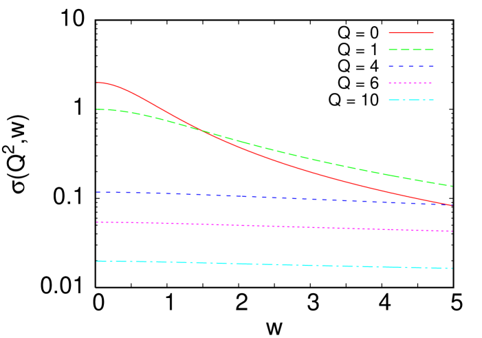
Figure 5: (Color online) Scaling function $\sigma(Q^{2},w)$ as a function of $w\equiv\omega\tau_{\rm int}(0)$, as obtained in one-loop perturbation theory.

Finally, in Fig. 5 we report the one-loop perturbative expression of $\sigma(Q^{2},w)$. Note that the width of $\sigma(Q^{2},w)$ does not decrease with increasing $Q^{2}$, as it does in the Gaussian model. This is a consequence of the large-$S$ behavior of $\Gamma(Q^{2},S)$, whose decay is independent of $Q^{2}$.

IV.3 Simulation details

In this section we study the critical dynamics of Hamiltonian (9) at $p=0.8$ in the high-temperature phase, with the purpose of determining the time-dependent spin-spin correlation function $\widetilde{G}(k,t)$ and the related dynamic structure factor $\widehat{G}(k,\omega)$. We perform simulations on lattices of size $L\leq 128$ in the range $0.275\leq\beta\leq 0.284$, corresponding to $4\lesssim\xi\lesssim 16$. For each disorder sample, we start from a random configuration, run 1000 Swendsen-Wang and 1000 Metropolis iterations for thermalization, and then $N_{\rm it}$ Metropolis sweeps [typically, we took $N_{\rm it}$ varying between $30\tau_{\rm int}(0)$ and $100\tau_{\rm int}(0)$]. The number of samples varies between 5000 and 20000. We measure the second-moment correlation length $\xi(\beta,L)$ defined in Eq. (31) and the correlation function $\widetilde{G}(k,t)$. As we did for the static structure factor, we determine $\widetilde{G}(k,t)$ as

$$\widetilde{G}(k,t)={1\over 3}\sum_{x,y,z}(e^{ikx}+e^{iky}+e^{ikz})\overline{\langle\sigma(0,0,0;0)\sigma(x,y,z;t)\rangle},$$ (72)

where the sum runs over the coordinates $(x,y,z)$ of the lattice sites; the time $t$ is expressed in units of Metropolis lattice sweeps.

Given $\widetilde{G}(k,t)$, we determine $\tau_{\rm int}(0)$. More precisely, we determine $\tau_{{\rm int},x}(0)$ with $x=5$, as defined by the self-consistent equation (46). As discussed above, this is a good autocorrelation time for any $x$; therefore, we use this quantity to obtain a high-temperature estimate of $z$. We have also determined $\tau_{{\rm int},x}(0)$ with $x=8$. The results for $x=5$ and $x=8$ are consistent within errors, indicating that we can take $\tau_{{\rm int},5}(0)$ as an estimate of $\tau_{\rm int}(0)$. We also consider the effective exponents $\tau_{{\rm exp},x}(0)$ defined by Eqs. (44) and (45) with $A(t)=\widetilde{G}(k=0,t)$. The results we quote correspond to $n=2$.

Table 1: MC results for the randomly site-diluted Ising model at $p=0.8$. We report the number of samples $N_{s}$, the number of Metropolis iterations in equilibrium $N_{\rm it}$, the second-moment correlation length $\xi$, the zero-momentum integrated autocorrelation time $\tau_{\rm int}(0)$, and the effective zero-momentum exponential autocorrelation times $\tau_{{\rm exp},x}(0)$, for $x=1,2$.

$\beta$	$L$	$N_{s}$	$N_{\rm it}$	$\xi$	$\tau_{\rm int}(0)$	$\tau_{{\rm exp},1}(0)$	$\tau_{{\rm exp},2}(0)$
0.275	32	$20000$	$30000$	4.452(4)	36.66(27)	37.92(18)	39.9(5)
0.278	32	$20000$	$5000$	5.601(4)	62.25(23)	65.70(25)	71.3(6)
	64	$20000$	$5000$	5.622(2)	61.98(21)	65.41(30)	69.4(9)
0.280	32	$20000$	$8000$	6.872(7)	102.1(6)	106.8(5)	118.2(1.2)
0.281	32	$20000$	$10000$	7.800(9)	139.4(7)	146.7(7)	164.1(1.7)
	64	$20000$	$5000$	7.917(4)	139.7(8)	148.2(7)	158(2)
	128	$10000$	$5000$	7.924(2)	138.8(1.0)	147.1(1.1)	157(3)
0.282	64	$15000$	$20000$	9.331(6)	207.0(1.0)	220(2)	238(3)
	128	$5000$	$20000$	9.346(5)	205.5(1.6)	218.8(1.3)	232(4)
0.283	64	$20000$	$20000$	11.551(10)	342.8(2.1)	361.0(1.6)	402(4)
0.284	128	$5000$	$50000$	15.837(16)	716(6)	753(9)	842(19)

Some results are reported in Table 1. Since we are interested in infinite-volume quantities, we must be sure that finite-size effects are negligible. A detailed check is performed at $\beta=0.281$, where we can compare simulation results at different values of $L$, corresponding to $\xi(\beta,L)/L\approx 0.24$, 0.12, and 0.06. No scaling corrections are observed in $\tau_{\rm int}(0)$ within the quoted errors, and thus, for each $\beta$, we assume that the estimate of $\tau_{\rm int}(0)$ for the largest lattices is an infinite-volume result. Also $\tau_{{\rm exp},1}(0)$ apparently does not show finite-size effects. On the other hand, $\tau_{{\rm exp},2}(0)$ is clearly decreasing as $L$ increases. This indicates that finite-size effects on $\widetilde{G}(k,t)$ increase with $t$, a result that we will check explicitly below, considering the correlation function.

IV.4 Dynamic structure factor

We first use the estimates of the autocorrelation times to obtain an estimate of $z$. Since the model is approximately improved,HPPV-07 the scaling corrections proportional to $(\beta_{c}-\beta)^{\omega\nu}$, $\omega=0.29(3)$ are suppressed. Thus, the leading scaling corrections behave as $(\beta_{c}-\beta)^{\omega_{2}\nu}$, where $\omega_{2}=0.82(8)$ is the next-to-leading correction-to-scaling exponent. Hence, $\tau(\beta)$ behaves as

$$\tau(\beta)\approx c(\beta_{c}-\beta)^{-z\nu}(1+b(\beta_{c}-\beta)^{\Delta_{2}}+\cdots),$$ (73)

where $\Delta_{2}=\nu\omega_{2}=0.56(6)$. Thus, we fit the data to

$$\ln\tau(\beta)=-z\nu\ln(\beta_{c}-\beta)+a+b(\beta_{c}-\beta)^{\Delta_{2}},$$ (74)

setting $\beta_{c}=0.2857431(3)$. HPPV-07 ; HPV-07 If we fit $\tau_{\rm int}(0)$, including only the data satisfying $\beta\geq\beta_{\rm min}$, we obtain $z\nu=1.64(3),1.59(4),1.62(8)$ for $\beta_{\rm min}=0.275$, 0.278, 0.280. The results are stable with $\beta_{\rm min}$ and allows us to estimate $z\nu=1.61(6)$ that includes all estimates with their error bars. If we now useHPPV-07 $\nu=0.683(2)$, we obtain

$$z=2.36(9),$$ (75)

which is in perfect agreement with the estimate $z=2.35(2)$ obtained at the critical point.HPV-07 As a check we have repeated the analysis by using $\tau_{{\rm exp},1}(0)$. We obtain $z\nu=1.59(3),1.56(5),1.47(10)$ for $\beta_{\rm min}=0.275$, 0.278, 0.280, which are essentially consistent with the estimates obtained above.

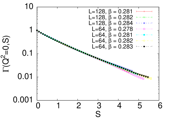
Figure 6: (Color online) Scaling function $\widetilde{G}(0,t)/\widetilde{G}(0,0)$ as a function of $S$, for different values of $\beta$ and $L$.

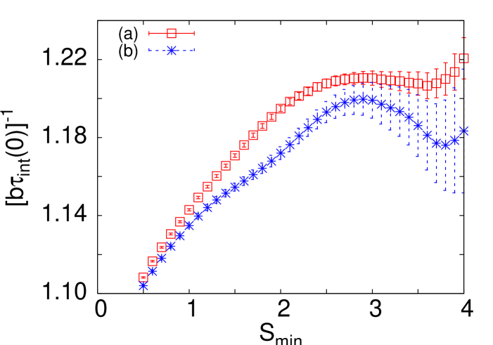
Figure 7: (Color online) Estimates of $[b\tau_{\rm int}(0)]^{-1}$, which converges to $f_{\rm exp}(0)$ in the critical limit. The coefficient $b$ is obtained by fitting $\widetilde{G}(0,t)/\widetilde{G}(0,0)$, as described in the text, see Eq. (76). In fit (a) we consider together the data corresponding to ($L=64$, $\beta=0.278$), ($L=128$, $\beta=0.281$), and ($L=128$, $\beta=0.282$). In fit (b) we only consider the results obtained for $L=128$, $\beta=0.281$.

Let us now consider $\widetilde{G}(k,t)$. Let us first focus on the case $k=Q=0$. Numerical results are reported in Fig. 6 vs $S\equiv t/\tau_{\rm int}(0)$. Scaling and finite-size corrections are small and indeed all data fall approximately onto a single curve. Some deviations are only observed for $S\gtrsim 3$, indicating that finite-size corrections increase with $S$. Let us now consider the large-$S$ behavior and let us estimate the universal ratio $f_{\rm exp}(0)$. The data show a reasonably good exponential behavior so that we can assume that we are considering values of $t$ that are much before the region in which $\widetilde{G}(0,t)$ shows the Griffiths tail. We perform fits of the form

$$\ln{\widetilde{G}(0,t)\over\widetilde{G}(0,0)}=a-bt,$$ (76)

including each time only data in the range $S_{\rm min}\leq S\leq S_{\rm max}\approx 5$. The fit parameter $b$ provides an estimate of $f_{\rm exp}(0)$: in the critical limit $f_{\rm exp}(0)=[b\tau_{\rm int}(0)]^{-1}$. Since finite-size corrections are important, we only consider data with small $\xi/L$. In Fig. 7 we report the results corresponding to two sets of data. In fit (a) we consider three sets of results: those corresponding to $L=64$, $\beta=0.278$ and those with $L=128$ and $\beta=0.281,0.282$. Correspondingly, we have $\xi(\beta,L)/L=0.088,0.061,0.073$, respectively. In fit (b) we only use the lattice with the smallest value of $\xi/L$ available: $L=128$ and $\beta=0.281$. The results of fit (a) become independent of $S_{\rm min}$ for $S_{\rm min}\gtrsim 2.5$ and give $f_{\rm exp}(0)=1.21(1)$. Fit (b) is less stable and a plateau is less evident. They hint at a lower value for the ratio, varying between 1.20 (at $S_{\rm min}=3$) and $1.18$ (at $S_{\rm min}=4$), though with a large statistical error. We have also analyzed the data corresponding to lattices with larger $\xi/L$, finding larger values of $[b\tau_{\rm int}(0)]^{-1}$. This indicates that this quantity decreases with decreasing $\xi(\beta,L)/L$ and thus the difference obtained between fits (a) and (b) may be a real finite-size effect. For this reason our final result corresponds to fit (b). We quote

$$f_{\rm exp}(0)=1.19(3),$$ (77)

where the error has been chosen conservatively, in order to include the result of fit (a) with its error. This result is very close to the one-loop FT estimate. Eq. (122) gives $f_{\rm exp}\approx 1.168$ for $\epsilon=1$.

Finally, we provide an interpolation of our numerical data. The curves reported in Fig. 6 are well fitted by a function of the form

$$\Gamma(0,S)=e^{-\kappa S}+\sum_{k=1}^{4}a_{k}{(cS)^{k}\over 1+(cS)^{4}e^{\kappa S}}.$$ (78)

The constant $\kappa$ has been fixed by using Eq. (77): we take $\kappa=0.840\approx 1/1.19$. All other constants have been obtained by a fit of the data for $0\leq S\leq 5$. We obtain $c=1.69$, $a_{1}=-0.23825$, $a_{2}=0.16430$, $a_{3}=0.13261$, $a_{4}=-0.28028$. As a check of this parametrization we verify the normalization conditions (50). The first condition is satisfied exactly, the second one to very good precision: the integral between 0 and infinity of $\Gamma(0,S)$ as given by the parametrization (78) is equal to 1.0033.

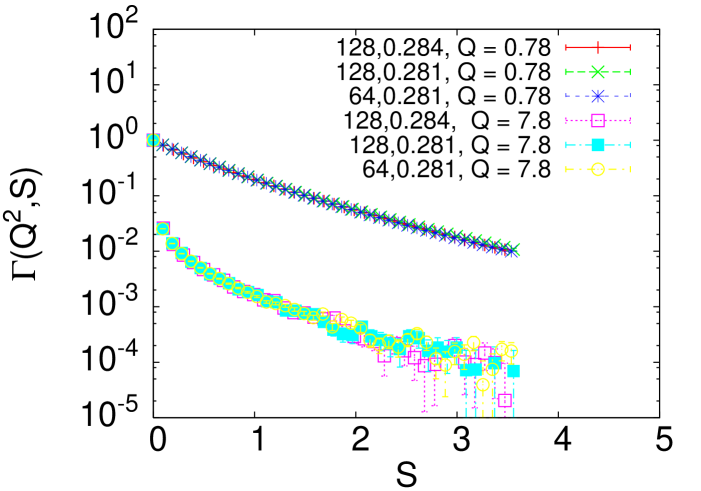
Figure 8: (Color online) Scaling function $\Gamma(Q^{2},S)$ as computed numerically for two values of $Q^{2}$. For each $Q$, we report results corresponding to three different values of $\beta$ and $L$.

Let us now consider $\widetilde{G}(k,t)$ for $k\not=0$. Again, let us first discuss the finite-size and scaling corrections. For this purpose, we must compare $\widetilde{G}(k,t)$ for different values of $\beta$ and $L$, but at the same value of $Q\equiv k\xi$. Since the momenta accessible on a finite lattice of size $L$ are quantized and therefore estimates are obtained only for $Q=2\pi n\xi/L$, $n$ integer, for each $t$ we should interpolate the numerical data as we did in Sec. III.3. However, by a fortunate accident, such an interpolation is not needed here. Indeed, the lattice with $L=64$, $\beta=0.281$ and that $L=128$, $\beta=0.284$ have both $\xi(\beta,L)/L=0.1237(1)$. Moreover, for $L=128$, $\beta=0.281$, $\xi/L$ is exactly 1/2 (within the small statistical errors) of the previous value. Thus, results with the same $k$ for the first two systems and those with $2k$ for the third one correspond quite precisely to the same value of $Q$. In Fig. 8 we report results corresponding to $Q=2\pi\times 0.1237\approx 0.78$ and $Q=20\pi\times 0.1237\approx 7.8$. All results fall again onto a single curve for both values of $Q$. Finite-size and scaling corrections are apparently negligible in this range of values of $Q$ and $S$. This result should be compared with what we observed for the static structure factor in Sec. III.3. There, a good scaling behavior was only observed at fixed $\widehat{Q}$ and not at fixed $Q$. Here instead, scaling corrections at fixed $Q$ are quite small; the behavior at fixed $\widehat{Q}$ is actually slightly worse.

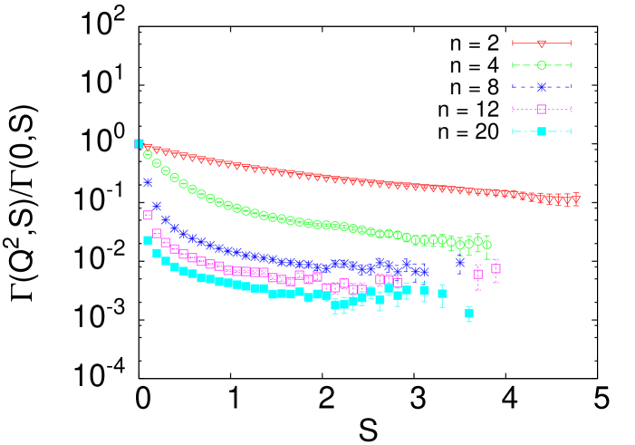
Figure 9: (Color online) Ratio $\widetilde{G}(k,t)/\widetilde{G}(0,t)\approx\Gamma(Q^{2},S)/\Gamma(0,S)$ obtained at $\beta=0.282$, $L=128$, versus $S$. Results correspond to different values of $Q^{2}=4\pi^{2}n^{2}\xi^{2}/L^{2}$. The values $n=2,4,8,12,20$ correspond to $Q^{2}\approx 0.84,3.37,13.5,30.3,84$.

An important prediction of the FT analysis is that $\Gamma(Q^{2},S)$ decays with the same rate for all values of $Q$. To check this prediction we consider the ratio $\widetilde{G}(k,t)/\widetilde{G}(0,t)$, which converges to $\Gamma(Q^{2},S)/\Gamma(0,S)$ in the scaling limit. For $S\to\infty$, this quantity should behave as

$$S^{\alpha}\exp\left[-S(f_{\rm exp}(Q^{2})^{-1}-f_{\rm exp}(0)^{-1})\right],$$ (79)

where $\alpha$ is some critical exponent. Field theory predicts $f_{\rm exp}(Q^{2})=f_{\rm exp}$ independent of $Q$, so that we expect $\Gamma(Q^{2},S)/\Gamma(0,S)$ to behave as $S^{\alpha}$ for large $S$, without exponential factors. Thus, if field theory is correct, $\ln[\widetilde{G}(k,t)/\widetilde{G}(0,t)]$ should become constant as $t$ increases, apart from possible slowly varying logarithmic corrections. In Fig. 9 we show this ratio for the lattice with $\beta=0.282$, $L=128$, which has been chosen because of its relatively small errors up to $S\approx 4$. The results for $\beta=0.284$, $L=128$, which are more asymptotic and give access to larger values of $Q$, are more noisy. The plot shows that the MC data are consistent with the FT prediction. Note that the constant behavior is observed better for larger values of $Q$. This is in agreement with the FT results shown in Fig. 4 and can be understood qualitatively quite easily. Roughly, at one loop $\Gamma(Q^{2},S)$ is the sum of two terms,

$$ae^{-S}+be^{-(1+Q^{2})S}$$ (80)

(we neglect here additional powers of $Q$ and $S$), so that the ratio we are considering corresponds to $(a+be^{-Q^{2}S})/(a+b)$. Thus, the ratio approaches a constant with corrections of order $e^{-Q^{2}S}$. For large $Q^{2}$ they die out fast, and thus a constant behavior is observed for small values of $S$.

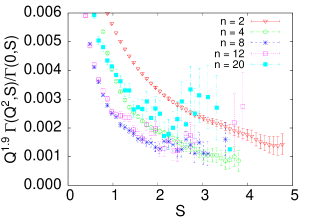
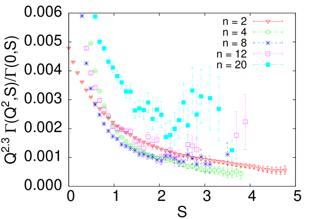
Figure 10: (Color online) Ratio $Q^{\zeta}\widetilde{G}(k,t)/\widetilde{G}(0,t)\approx Q^{\zeta}\Gamma(Q^{2},S)/\Gamma(0,S)$ obtained at $\beta=0.282$, $L=128$, versus $S$. Results correspond to different values of $Q^{2}=4\pi^{2}n^{2}\xi^{2}/L^{2}$. The values $n=2,4,8,12,20$ correspond to $Q^{2}\approx 0.84,3.37,13.5,30.3,84$. The figure on the left corresponds to $\zeta=1.9$, that on the right to $\zeta=2.3$.

While the decay rate of $\Gamma(Q^{2},S)$ is independent of $Q^{2}$, the amplitude decreases rapidly with $Q^{2}$. For large $Q^{2}$ we expect the behavior $\Gamma(Q^{2},S)\sim S^{a}Q^{-\zeta}\exp(-\kappa S)$, where $\kappa=1/f_{\rm exp}$, see Eq. (68). We wish now to obtain a rough estimate of the exponent $\zeta$. For this purpose we take the data that appear in Fig. 9 and we multiply them by $Q^{\zeta}$, trying to fix $\zeta$ in such a way to obtain a good collapse of the data. In Fig. 9 we report the scaled results corresponding to two different values of $\zeta$. If we try to have a good collapse of the data corresponding to $n=4,8,12$ the best result is obtained for $\zeta=2.3$. However, the data with $n=20$ behave in a significantly different way. If we try to include also the data with $n=20$, the quality of the collapse worsens and the best result is obtained for $\zeta=1.9$. These results indicate that $\zeta\approx 2$ (but with a large error), so that $\Gamma(Q^{2},S)$ behaves roughly as $Q^{-2}S^{a}\exp(-\kappa S)$. It is interesting to observe that this is exactly the behavior predicted close to four dimensions by perturbation theory.

Table 2: Numerical values of the coefficients appearing in the interpolation formula (81).

	$Q^{2}=0.842$	$Q^{2}=5.262$	$Q^{2}=21.05$	$Q^{2}=47.36$
$a_{0}$	$-$2.30388	0.0972492	$-$0.1390160	$-$0.1482217
$a_{1}$	1.85440	$-$0.1867741	$-$0.0166780	0.0609449
$a_{2}$	$-$1.03426	0.2245075	0.0882145	$-$0.0108184
$a_{3}$	$-$1.04434	$-$0.0670895	$-$0.0483811	$-$0.0040681
$a_{4}$	2.29488	$-$0.0788428	0.1494524	0.1510844
$d_{0}$	3.30388	0.9027518	1.1390167	1.1482211
$d_{1}$	$-$1.87228	$-$0.5008092	$-$13.808512	$-$19.439356
$d_{2}$	2.03391	12.846119	114.32824	182.53584
$d_{3}$	$-$0.64676	$-$27.878988	$-$319.65479	$-$587.00842
$d_{4}$	0.13949	58.784027	519.97023	1021.6385
$\kappa_{2}$	1.95	9.08	10.46	12.40
$c$	2.000	1.124	1.087	1.282

Finally, we determine an interpolation formula for $\Gamma(Q^{2},S)$. We find that all data are well fitted by taking

$$\Gamma(Q^{2},S)=a_{0}e^{-\kappa_{1}S}+\sum_{k=1}^{4}a_{k}{(cS)^{k}\over 1+(cS)^{4}e^{\kappa_{1}S}}+\sum_{k=0}^{4}d_{k}S^{k}e^{-\kappa_{2}S},$$ (81)

fixing $\kappa_{1}=0.840$. The results of the fits for a few chosen values of $Q^{2}$ are reported in Table 2. We have not required $a_{0}+d_{0}=1$, a condition that follows from $\Gamma(Q^{2},S=0)=1$, but we have verified that the results satisfy this condition quite precisely. By using a linear interpolation, the results we report should allow the reader to determine $\Gamma(Q^{2},S)$ for any $Q$ in the range $0\leq Q^{2}\leq 50$ with reasonable precision. We stress that this interpolation formula only represents a compact expression that summarizes the numerical results. The chosen parametrization has indeed a purely phenomenological value.

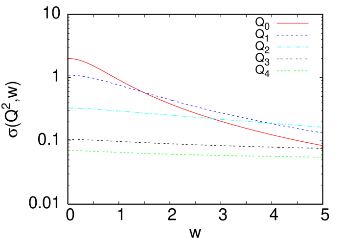
Figure 11: (Color online) Numerical estimate of the scaling function $\sigma(Q^{2},w)$ as a function of $w\equiv\omega\tau_{\rm int}(0)$, as obtained by integrating the interpolating expression (81). The values of the momenta are: $Q_{0}=0$, $Q_{1}^{2}=0.842$, $Q_{2}^{2}=5.262$, $Q_{3}^{2}=21.05$, $Q_{4}^{2}=47.36$.

From these expressions it is easy to determine the scaling function $\sigma(Q^{2},w)$ related to the dynamic structure factor. In Fig. 11 we plot the scaling function $\sigma(Q^{2},w)$ as obtained by integrating the interpolating function determined above. We report it for the same values of $Q^{2}$ that appear in Table 2. The qualitative behavior is in full agreement with the FT prediction, compare with Fig. 5. Quantitatively, perturbation theory is also reasonably predictive. For $Q=0$ and $w<5$, the relative differences between the FT and the numerical expression are less than 2%. For larger values of $Q^{2}$ differences increase: for instance, for the values of $Q$ that appear in Fig. 11, field theory predicts $\sigma(Q^{2},0)\approx 2$, 1.09, 0.32, 0.091, 0.041, while we obtain numerically $\sigma(Q^{2},0)\approx 2$, 1.09, 0.33, 0.105, 0.072. These discrepancies are probably the fault of both field theory—after all, we are at one loop—and of the numerical results—for large $Q$ the data are noisy and the estimates have a large error. In any case this comparison indicates that, up to $Q=5$, errors are under control and the reported expressions are precise enough for all practical purposes.

Appendix A Perturbative results for the static structure factor

The static behavior of Ising systems with random dilution can be studied starting from the Landau-Ginzburg-Wilson Hamiltonian GL-76

$${\cal H}=\int d^{d}x\left[{1\over 2}(\partial_{\mu}\varphi)^{2}+{1\over 2}r\varphi^{2}+{1\over 2}\psi\varphi^{2}+{1\over 4!}g_{0}\varphi^{4}\right],$$ (82)

where $\psi(x)$ is a spatially uncorrelated random field with Gaussian distribution

$$P(\psi)={1\over\sqrt{4\pi w}}\exp\left[-{\psi^{2}\over 4w}\right].$$ (83)

Using the standard replica trick, it is possible to replace the quenched average with an annealed one. As a result of this procedure, one can investigate the static critical behavior of RDI systems by applying standard FT methods to the Hamiltonian GL-76

$${\cal H}_{\rm replica}=\int d^{d}x\Bigl{\{}\sum_{i}{1\over 2}\left[(\partial_{\mu}\phi_{i})^{2}+r\phi_{i}^{2}\right]+\sum_{ij}{1\over 4!}\left(u_{0}+g_{0}\delta_{ij}\right)\phi^{2}_{i}\phi^{2}_{j}\Bigr{\}},$$ (84)

where $i,j=1,...N$ and $u_{0}=-6w$. RDI results are obtained by taking the limit $N\to 0$.

A.1 $\sqrt{\epsilon}$-expansion results

The scaling function $g(Q^{2})$ can be determined by using the results reported in Ref. CPRV-98, . We obtain the expansion

$$g(y)^{-1} = 1+y-\epsilon\frac{1}{53}\psi_{2}(y)+18\frac{\sqrt{6/53}}{2809}[24+7\zeta(3)]\epsilon^{3/2}\psi_{2}(y)+O(\epsilon^{2})$$ (85)

$$= 1+y-0.0188679\epsilon\psi_{2}(y)+0.069887\epsilon^{3/2}\psi_{2}(y)+O(\epsilon^{2})\,,$$

where $\psi_{2}(y)$ is the two-loop contribution defined in Ref. CPRV-98, . Note that the only relevant three-loop diagram contributes only at order $\epsilon^{5/2}$ (hence, at five loops), since it is proportional to

$${1\over 27}(u+3v)(4u+3v)^{2},$$ (86)

and, at the fixed point, $4u^{*}+3v^{*}$ is of order $\epsilon$ and not of order $\sqrt{\epsilon}$.

The expansion of $\psi_{2}(y)$ for small $y$ can be found in Ref. CPRV-98, . It allows us to obtain the expansions

$$c_{2} = 0.000141891\epsilon-0.000525567\epsilon^{3/2}+O(\epsilon^{2}),$$

$$c_{3} = -3.62134\cdot 10^{-6}\epsilon+0.0000134135\epsilon^{3/2}+O(\epsilon^{2}),$$

$$c_{4} = 1.53623\cdot 10^{-7}\epsilon-5.69021\cdot 10^{-7}\epsilon^{3/2}+O(\epsilon^{2}),$$

$$c_{5} = -8.28575\cdot 10^{-9}\epsilon+3.06905\cdot 10^{-8}\epsilon^{3/2}+O(\epsilon^{2}).$$ (87)

The expansion of $\psi_{2}(y)$ for large values of $y$ is Bray-76

$$\psi_{2}(y)=-\frac{1}{4}y\log y+2Q_{0}y-\frac{3}{4}\log^{2}y+2Q_{1}+\dots$$ (88)

with $Q_{0}\approx 0.507826$ and $Q_{1}\approx 0.1289$. Matching the large-momentum expansion of Eq. (85) with the Fisher-Langer behavior (20) we obtain the expansions of the coefficients $C_{i}$:

$$C_{1}=1+0.0191632\epsilon-0.0709809\epsilon^{3/2}+O(\epsilon^{2}),$$

$$C_{2}=-1/2-0.757042\epsilon^{1/2}+1.34297\epsilon+c_{2,3}\epsilon^{3/2}+O(\epsilon^{2}),$$

$$C_{3}=-1/2+0.757042\epsilon^{1/2}-1.35726\epsilon+c_{3,3}\epsilon^{3/2}+O(\epsilon^{2}),$$ (89)

where $c_{2,3}+c_{3,3}=0.052964$. Setting $\epsilon=1$, we obtain $C_{1}\approx 0.95$, $C_{2}+C_{3}=-0.96$.

A.2 Massive zero-momentum results

We have determined the low-momentum behavior of $g(Q^{2})^{-1}$ in the MZM scheme by using the perturbative results of Ref. CPRV-98, . The four-loop expansions of the first few coefficients $c_{n}$ are:

$$c_{2}= -{1\over 6480}u^{2}-{1\over 2430}uv-{2\over 10935}v^{2}-0.0000120404u^{3}-0.0000481617u^{2}v$$

$$-0.0000481617uv^{2}-0.0000142701v^{3}-0.00000718972u^{4}-0.0000383452u^{3}v$$

$$-0.0000617074u^{2}v^{2}-0.0000379116uv^{3}-0.00000842479v^{4},$$

$$c_{3}= {1\over 122472}u^{2}+{1\over 45927}uv+{4\over 413343}v^{2}-0.00000281924u^{3}-0.0000112769u^{2}v$$

$$-0.0000112769uv^{2}-0.00000334132v^{3}+0.00000660026u^{4}+0.00000352014u^{3}v$$

$$+0.00000562891u^{2}v^{2}+0.00000339371uv^{3}+0.000000754158v^{4},$$

$$c_{4}= -{1\over 1889568}u^{2}-{1\over 708588}uv-{1\over 1594323}v^{2}+0.000000347995u^{3}+0.00000139198u^{2}v$$ (90)

$$+0.00000139198uv^{2}+0.000000412438v^{3}-0.000000141114u^{4}-0.000000752609u^{3}v$$

$$-0.00000119627u^{2}v^{2}-0.000000740733uv^{3}-0.000000164607v^{4}.$$

The MZM renormalized quartic couplings $u$ and $v$ are normalized so that at tree level $u=u_{0}/m$ and $v=v_{0}/m$. Their fixed-point values are $u^{*}=-18.6(3)$ and $v^{*}=43.3(2)$ (obtained by means of MC simulations CMPV-03 ), and $u^{*}=-13.5(1.8)$ and $v^{*}=38.0(1.5)$ (obtained by resumming the six-loop $\beta$-function PV-00 ).

Appendix B One-loop calculation of the response and correlation functions

The relaxational model-A dynamics is described by the stochastic Langevin equation HH-77

$$\frac{\partial\varphi(r,t)}{\partial t}=-\Omega\frac{\delta\cal{H}(\varphi)}{\delta\varphi(r,t)}+\zeta(r,t),$$ (91)

where $\varphi(r,t)$ is the order parameter, $\cal{H}(\varphi)$ is the Hamiltonian (82), $\Omega$ is a transport coefficient, and $\zeta(r,t)$ is a Gaussian random field (white noise) with correlations

$$\langle\zeta(r,t)\rangle=0,\qquad\langle\zeta(r_{1},t_{1})\zeta(r_{2},t_{2})\rangle=\Omega\delta(r_{1}-r_{2})\delta(t_{1}-t_{2}).$$ (92)

The correlation functions generated by the Langevin equation (91) at equilibrium, averaged over the noise $\zeta$ and the quenched disorder $\psi$, can be obtained from the FT action DeDominicis-78

$$S(\varphi,\hat{\varphi})= \int d^{d}x\left[\int dt\,\hat{\varphi}(\partial_{t}\varphi-\Omega\Delta\varphi-\Omega\hat{\varphi}+\Omega r\varphi)\right.$$

$$\left.+{\Omega g_{0}\over 3!}\int dt\,\hat{\varphi}\varphi^{3}+{\Omega^{2}u_{0}\over 6}\left(\int dt\,\hat{\varphi}\varphi\right)^{2}\right],$$

where $\hat{\varphi}$ is the response field. In this framework, no replicas are introduced. DeDominicis-78 We consider the correlation function $G(x,t)$ and the response function $R(x,t)$ defined by

$$G(x_{2}-x_{1},t_{2}-t_{1})=\langle\varphi(x_{1},t_{1})\varphi(x_{2},t_{2})\rangle,$$ (94)

$$R(x_{2}-x_{1},t_{2}-t_{1})=\langle\hat{\varphi}(x_{1},t_{1})\varphi(x_{2},t_{2})\rangle,$$ (95)

and their spatial Fourier transforms $\widetilde{G}(k,t)$ and $\widetilde{R}(k,t)$. In equilibrium, they are not independent, but related by the fluctuation-dissipation theorem; for $t>0$ they satisfy the relation $\partial_{t}G(x,t)=-\Omega R(x,t)$. For a general introduction to the FT approach to equilibrium critical dynamics, see, e.g., Refs. FM-06, ; CG-05, . Some perturbative calculations can be also found in Refs. pertcalc, .

B.1 One-loop calculation

Figure 12: The one-loop graphs contributing to the response function. We indicate with $L_{g}(k,t)$ and with $L_{u}(k,t)$ the contribution of the graph on the left and on the right, respectively.

We first compute the response function $\widetilde{R}(k,t)$ and then use the fluctuation-dissipation theorem to derive the correlation function $\widetilde{G}(k,t)$. At one-loop we obtain in dimensional regularization

$$\widetilde{R}(k,t)=\widetilde{R}_{G}(k,t)-{g_{0}\over 2}L_{g}(k,t)-{u_{0}\over 3}L_{u}(k,t)+O(u_{0}^{2},u_{0}g_{0},g_{0}^{2}),$$ (96)

where

$$\widetilde{R}_{G}(k,t)=\theta(t)\exp[-\Omega(k^{2}+r)t]$$ (97)

is the Gaussian tree-level response function, and $L_{u}(k,t)$ and $L_{g}(k,t)$ are the one-loop contributions, see Fig. 12. It is straightforward to obtain

$$L_{g}(k,t) = \Omega\int_{-\infty}^{\infty}ds\int{d^{d}q\over(2\pi)^{d}}\,\widetilde{R}_{G}(k,t-s)\widetilde{R}_{G}(k,s)\widetilde{G}_{G}(q,0)$$ (98)

$$= -{N_{d}\over\epsilon}r^{1-\epsilon/2}\Omega t\widetilde{R}_{G}(k,t),$$

where $\epsilon\equiv 4-d$, $N_{d}\equiv 2/[\Gamma(d/2)(4\pi)^{d/2}]$, and $\widetilde{G}_{G}(k,t)$ is the Gaussian tree-level correlation function (59). Analogously, we obtain

$$L_{u}(k,t)=\Omega^{2}\int_{-\infty}^{\infty}ds_{1}\int_{-\infty}^{\infty}ds_{2}\int{d^{d}q\over(2\pi)^{d}}\,\widetilde{R}_{G}(k,t-s_{2})\widetilde{R}_{G}(q,s_{2}-s_{1})\widetilde{R}_{G}(k,s_{1})$$

$$={N_{d}\over\epsilon}(1+\epsilon\gamma_{E}/2)(\Omega t)^{\epsilon/2}(\Omega tk^{2}-1)\widetilde{R}_{G}(k,t)+\theta(t){1\over(4\pi)^{2}}e^{-\Omega tr}F(\Omega tk^{2})+O(\epsilon),$$ (99)

where

$$F(x)\equiv-1+e^{-x}+e^{-x}(x-1)[{\rm Ei}(x)-\gamma_{E}-\ln x],$$ (100)

and ${\rm Ei}(x)$ is the exponential integral function.

Renormalizing the response function in the $\overline{\rm MS}$ scheme we obtain

$$\widetilde{R}(k,t) = \widetilde{R}_{G}(k,t)-{g\over 32\pi^{2}}\Omega tr\ln r\widetilde{R}_{G}(k,t)$$ (102)

$$-{u\over 48\pi^{2}}(\gamma_{E}+\ln\Omega t)(\Omega tk^{2}-1)\widetilde{R}_{G}(k,t)-{u\over 48\pi^{2}}\theta(t)e^{-\Omega tr}F(\Omega tk^{2}),$$

where $r,\Omega,u,g$ are renormalized parameters (note that we use the same symbols $r$ and $\Omega$ for both the bare and the renormalized parameters, since no confusion can arise). The final expression is obtained by setting $g$ and $u$ equal to their fixed-point values:

$$g^{*}=32\pi^{2}\sqrt{{6\epsilon\over 53}},\qquad u^{*}=-24\pi^{2}\sqrt{{6\epsilon\over 53}}.$$ (103)

The correlation function $\widetilde{G}(k,t)$ for $t>0$ can be obtained from

$$\widetilde{G}(k,t)=\Omega\int_{t}^{\infty}\widetilde{R}(k,t),$$ (104)

which follows from the fluctuation-dissipation theorem and the fact that $\widetilde{G}(k,t)\to 0$ as $t\to\infty$. A straightforward calculation gives (in the following we always assume $t>0$)

$${\widetilde{G}(k,t)\over\widetilde{G}(k,0)} = e^{-\Omega t(k^{2}+r)}-{g\over 32\pi^{2}}\Omega tr(\ln r)e^{-\Omega t(k^{2}+r)}$$ (105)

$$-{u\over 48\pi^{2}}(\gamma_{E}+\ln\Omega t)\Omega tk^{2}e^{-\Omega t(k^{2}+r)}-{u\over 48\pi^{2}}\left(e^{-\Omega t(k^{2}+r)}-e^{-\Omega tr}\right)$$

$$-{u\over 48\pi^{2}}\left(\Omega tk^{2}-{r\over k^{2}+r}\right)e^{-\Omega t(k^{2}+r)}\left({\rm Ei}(\Omega tk^{2})-\gamma_{E}-\ln\Omega tk^{2}\right)$$

$$-{u\over 48\pi^{2}}{r\over k^{2}+r}\left[{\rm Ei}(-\Omega tr)-e^{-\Omega t(k^{2}+r)}(\gamma_{E}+\ln\Omega tr)\right],$$

where

$$\widetilde{G}(k,0)={1\over k^{2}+r}-{1\over 32\pi^{2}}(g+2u/3){r\ln r\over(k^{2}+r)^{2}}.$$ (106)

It is easy to derive the critical correlation function at one-loop order from Eq. (105). Taking the limit $r\to 0$, we obtain

$${\widetilde{G}(k,t)\over\widetilde{G}(k,0)} = e^{-\Omega tk^{2}}-{u\over 48\pi^{2}}(\gamma_{E}+\ln\Omega t)\Omega tk^{2}e^{-\Omega tk^{2}}-{u\over 48\pi^{2}}\left(e^{-\Omega tk^{2}}-1\right)$$ (107)

$$-{u\over 48\pi^{2}}\Omega tk^{2}e^{-\Omega tk^{2}}\left({\rm Ei}(\Omega tk^{2})-\gamma_{E}-\ln\Omega tk^{2}\right).$$

In the critical limit the correlation function should only depend on the scaling variable $K^{2}\equiv k^{2}(\Omega t)^{2/z}$. Keeping into account that $z=2-u/(24\pi^{2})$ at one loop, we obtain at this order (we set $u=u^{*}$)

$${\tilde{G}(k,t)\over\tilde{G}(k,0)} = e^{-K^{2}}-{u^{*}\over 48\pi^{2}}\left(e^{-K^{2}}-1\right)-{u^{*}\over 48\pi^{2}}K^{2}e^{-K^{2}}\left({\rm Ei}(K^{2})-\ln K^{2}\right).$$ (108)

This scaling function has a regular expansion in powers of $K^{2}$ for $K\to 0$, while, for $K\to\infty$, it behaves as

$${\widetilde{G}(k,t)\over\widetilde{G}(k,0)} \approx -{u^{*}\over 48\pi^{2}K^{2}}={1\over 2K^{2}}\sqrt{6\epsilon\over 53}.$$ (109)

Given Eq. (108), we can compute $G(x,t)$ at the critical point. We expect the scaling behavior

$$G(x,t)=(\Omega t)^{-(d+\eta-2)/z}F(X),\qquad\qquad X\equiv x(\Omega t)^{-1/z}.$$ (110)

Using Eq. (108) we obtain

$$F(X)={1\over 4\pi^{2}X^{2}}(1-e^{-X^{2}/4})-{u^{*}\over 48\pi^{2}}F_{\rm 1\,loop}(X),$$ (111)

with

$$F_{\rm 1\,loop}(X)={1\over 4\pi^{2}X}\int_{0}^{\infty}dK\,J_{1}(KX)\left[e^{-K^{2}}-1+K^{2}e^{-K^{2}}\left({\rm Ei}(K^{2})-\ln K^{2}\right)\right],$$ (112)

where $J_{1}(x)$ is a Bessel function. In the derivation we have taken into account that $u\sim\sqrt{\epsilon}$. It is interesting to note that $F_{\rm 1\,loop}(X)$ is not regular for $X\to 0$. Indeed, the explicit calculation gives

$$F_{\rm 1\,loop}(X) = -{1\over 16\pi^{2}}\ln{X^{2}\over 4}+O(X^{2}\ln X^{2}).$$ (113)

This result indicates that $F(X)$ is not regular for $X\to 0$, but behaves as

$$F(X)\approx a_{0}+b_{0}|X|^{\lambda}+\cdots$$ (114)

where $\lambda$ is a critical exponent. Comparing this expression with Eqs. (111) and (113) we obtain

$$a_{0}+b_{0}={1\over 16\pi^{2}}+O(\sqrt{\epsilon}),$$ (115)

$$b_{0}\lambda={u^{*}\over 384\pi^{4}}+O(\epsilon)=-{1\over 16\pi^{2}}\sqrt{6\epsilon\over 53}+O(\epsilon).$$ (116)

It is not possible to compute $\lambda$, $a_{0}$, and $b_{0}$ separately at this order. A two-loop computation of the term proportional to $\epsilon\ln^{2}X$ is needed.

In the high-temperature phase, it is convenient to replace $r$ and $\Omega$ with the correlation length $\xi$ and the zero-momentum integrated autocorrelation time $\tau_{\rm int}(k=0)$, defined in Sec. III.1 and IV.1, respectively. A tedious calculation gives

$$\xi^{-2} = r+{1\over 32\pi^{2}}(g+2u/3)r\ln r,$$ (117)

$$\Omega\tau_{\rm int}(k) = {1\over k^{2}+r}-{g\over 32\pi^{2}}{r\ln r\over(k^{2}+r)^{2}}+{u\over 48\pi^{2}}{k^{2}\ln r\over(k^{2}+r)^{2}}+{u\over 48\pi^{2}}{1\over k^{2}+r}.$$ (118)

Using these results, we obtain the one-loop expression of the scaling function $\Gamma(Q^{2},S)$:

$$\Gamma(Q^{2},S) = e^{-S(Q^{2}+1)}-{u^{*}\over 48\pi^{2}}S(Q^{2}+1)e^{-S(Q^{2}+1)}$$ (119)

$$-{u^{*}\over 48\pi^{2}}(\gamma_{E}+\ln S)SQ^{2}e^{-S(Q^{2}+1)}-{u^{*}\over 48\pi^{2}}\left(e^{-S(Q^{2}+1)}-e^{-S}\right)$$

$$-{u^{*}\over 48\pi^{2}}\left(Q^{2}S-{1\over Q^{2}+1}\right)e^{-S(Q^{2}+1)}\left({\rm Ei}(SQ^{2})-\gamma_{E}-\ln SQ^{2}\right)$$

$$-{u^{*}\over 48\pi^{2}}{1\over Q^{2}+1}\left[{\rm Ei}(-S)-e^{-S(Q^{2}+1)}(\gamma_{E}+\ln S)\right],$$

where $u^{*}$ is the fixed-point value (103) of $u$.

It is interesting to discuss the large-$S$ and small-$S$ behavior of the scaling function (119). For large $S$ we obtain

$$\Gamma(Q^{2},S)\approx e^{-S(1+Q^{2})}-{u^{*}\over 48\pi^{2}}{1+Q^{2}\over(Q^{2})^{2}}{e^{-S}\over S^{2}}-{u^{*}\over 48\pi^{2}}(1+Q^{2}-Q^{2}\ln Q^{2})Se^{-S(1+Q^{2})}.$$ (120)

For $Q^{2}=0$ the dominant term is the last one. In this case we can rewrite the large-$S$ behavior as

$$\Gamma(Q^{2},S)\approx\exp\left[-S\left(1+{u^{*}\over 48\pi^{2}}\right)\right],$$ (121)

which gives for the exponential autocorrelation-time scaling function [see Eq. (52)]

$$f_{\rm exp}(0)=1-{u^{*}\over 48\pi^{2}}=1+{1\over 2}\sqrt{6\epsilon\over 53}+O(\epsilon).$$ (122)

For $Q^{2}\not=0$, the dominant term is the second one, so that for any $Q^{2}$ the scaling function decays as $e^{-S}/S^{2}$. Thus, at this perturbative order, we obtain the result

$$f_{\rm exp}(Q^{2})=1+O(\sqrt{\epsilon}).$$ (123)

The correlation function $\Gamma(Q^{2},S)$ decays with the same rate for all values of $Q$. As we discuss in Sec. IV.2, this is a consequence of the loss of translational invariance in dilute systems.

Equation (123) should be contrasted with the result obtained for the integrated autocorrelation times. Using Eq. (118), we obtain

$${\tau_{\rm int}(k)\over\tau_{\rm int}(0)}=f_{\rm int}(Q^{2})={1\over Q^{2}+1},$$ (124)

without one-loop corrections. This shows that $\tau_{\rm int}(k)$ decreases as $Q$ increases as it does in the Gaussian model.

Let us now consider the limit $S\to 0$. The scaling function has an expansion of the form

$$\Gamma(Q^{2},S)=1+\sum_{n=1}S^{n}(a_{n}+b_{n}\ln S).$$ (125)

Note the presence of terms proportional to $\ln S$. They should be generically expected, since in the critical limit (it corresponds to $Q\to\infty$ and $S\to 0$), the correlation function depends on

$$k^{2}(\Omega t)^{2/z}\sim Q^{2}S^{2/z}\sim Q^{2}S\left(1+{u^{*}\over 48\pi^{2}}\ln S\right).$$ (126)

The presence of these logarithms implies that the function $\Gamma(Q^{2},S)$ is not analytic for $S\to 0$.

It is also important to discuss the large-momentum behavior of $\Gamma(Q^{2},S)$. For $Q^{2}\to\infty$ the tree-level term vanishes exponentially as $e^{-SQ^{2}}$, while the one-loop term decays only algebraically, as $1/Q^{2}$. More precisely, for $Q^{2}\to\infty$ we have

$$\Gamma(Q^{2},S)\approx-{u^{*}\over 48\pi^{2}}\left({e^{-S}\over S}+{\rm Ei}(-S)\right)Q^{-2}.$$ (127)

The presence of these slowly decaying terms implies the singularity of the behavior of $G(x,t)$ for $x\to 0$ and for any $t$. In the critical limit we expect the scaling behavior (70), i.e., $G(x,t)=\xi^{-d+2-\eta}F(Y^{2},S)$, with $Y^{2}\equiv x^{2}/\xi^{2}$. We obtain for $Y\to 0$

$$F(Y^{2},S)\approx{1\over 16\pi^{2}}\left({e^{-S}\over S}+{\rm Ei}(-S)\right)\left(1+{u^{*}\over 24\pi^{2}}\ln Y\right)+u^{*}f_{\rm corr}(S)+\cdots$$ (128)

for $Y\to 0$, where $f_{\rm corr}(S)$ is a function of $S$. The presence of a term proportional to $\ln Y$ implies that $F(Y^{2},S)$ is not analytic as $Y\to 0$, i.e. has a behavior of the form $F(Y^{2},S)=f_{0}(S)+f_{\lambda}(S)|Y|^{\lambda}+\cdots$, where $\lambda$ is the same exponent that appears in Eq. (114). Note that Eq. (128) is apparently consistent with the assumption that $f_{0}(S)=0$. If this were the case, we would obtain

$$\lambda={u^{*}\over 24\pi^{2}}=-\sqrt{6\epsilon\over 53}+O(\epsilon).$$ (129)

This result would imply $\lambda<0$ and thus $F(Y^{2},S)$ would diverge as $Y\to 0$ for any $S$, at least for $\epsilon$ small. This behavior is clearly unphysical; thus, $f_{0}(S)$ should be nonvanishing.

The critical limit is obtained by taking $S\to 0$. Requiring the limiting function to be of the form (110), we obtain

$$f_{0}(S)\sim S^{(2-\eta-d)/z},$$

$$f_{\lambda}(S)\sim S^{(-\lambda+2-\eta-d)/z},$$ (130)

for $S\to 0$. The $S$-dependent prefactor appearing in Eq. (128) behaves as $1/S$ for $S\to 0$, which is consistent with these expressions.

The nonanalytic behavior of $F(Y^{2},S)$ as $Y\to 0$, implies that $\Gamma(Q^{2},S)$ should decay as a power of $Q$ as $Q\to\infty$. A simple calculation gives

$$\Gamma(Q^{2},S)\sim f_{\lambda}(S)Q^{2-d-\lambda-\eta},$$ (131)

for $Q^{2}\to\infty$. The exponent $\zeta$ defined in Eq. (69) is given by

$$\zeta=\lambda+d+\eta-2=2+O(\sqrt{\epsilon}).$$ (132)

Finally, we report $\sigma(Q^{2},w)$, cf. Eq. (56). A long calculation gives

$$\sigma(Q^{2},w) = {2\alpha\over\alpha^{2}+w^{2}}+{u^{*}\over 24\pi^{2}}\left\{{\alpha(\alpha^{2}-w^{2}+2\alpha w^{2})\over w(\alpha^{2}+w^{2})^{2}}{\rm Arctan}\,w+{\alpha(\alpha^{2}-w^{2}-2\alpha)\over 2(\alpha^{2}+w^{2})^{2}}\ln(1+w^{2})\right.$$ (133)

$$\left.+{1\over w^{2}+1}+{(w^{2}-\alpha)Q^{2}\over(w^{2}+1)(\alpha^{2}+w^{2})}-{2\alpha^{3}\over(\alpha^{2}+w^{2})^{2}}\right\},$$

where $\alpha\equiv 1+Q^{2}$.

For large $w$, $\sigma(Q^{2},w)$ behaves as

$$\sigma(Q^{2},w)\approx{2\alpha\over w^{2}}\left[1+{u^{*}\over 48\pi^{2}}(1-\ln w)\right],$$ (134)

which is compatible with the expected behavior $w^{-(2-\eta+z)/z}$.

Note also that the singularities of $\sigma(Q^{2},w)$ in the complex $w$-plane that are closest to the origin are $w=\pm i$, independently of $Q^{2}$. This is a direct consequence of the fact we have already noticed that the large-$t$ behavior is momentum independent. As a consequence, the width of the structure factor does not decrease with $Q^{2}$ as it does in pure systems.

References

- (1) D. P. Belanger, Braz. J. Phys. 30, 682 (2000); cond-mat/0009029.
- (2) A. Pelissetto and E. Vicari, Phys. Rept. 368, 549 (2002).
- (3) R. Folk, Yu. Holovatch, and T. Yavors’kii, Uspekhi Fiz. Nauk 173, 169 (2003) [English translation, Phys. Usp. 46, 175 (2003)].
- (4) P. C. Hohenberg and B. I. Halperin, Rev. Mod. Phys. 49, 435 (1977).
- (5) In Born approximation the static and dynamic structure factors are proportional to the elastic and inelastic cross section, respectively; and are respectively proportional to the transferred momentum and energy.
- (6) R. B. Griffiths, Phys. Rev. Lett. 23, 17 (1969); M. Schwartz, Phys. Rev. B 18, 2364 (1978).
- (7) T. Vojta, J. Phys. A 39, R143 (2006).
- (8) A. J. Bray, Phys. Rev. Lett. 60, 720 (1988).
- (9) D. Dhar, M. Randeria, and J. P. Sethna, Europhys. Lett. 5, 485 (1988).
- (10) A. J. Bray, J. Phys. A 22, L81 (1989).
- (11) F. Cesi, C. Maes, and F. Martinelli, Comm. Math. Phys. 188, 135 (1997); ibid. 189, 323 (1997).
- (12) M. B. Salamon, P. Lin, and S. H. Chun, Phys. Rev. Lett. 88, 197203 (2002); J. Deisenhofer, D. Braak, H.-A. Krug von Nidda, J. Hemberger, R. M. Eremina, V. A. Ivanshin, A. M. Balbashov, G. Jug, A. Loidl, T. Kimura, and Y. Tokura, Phys. Rev. Lett. 95, 257202 (2005); P. Y. Chan, N. Goldenfeld, and M. Salamon, Phys. Rev. Lett. 97, 137201 (2006); C. Magen, P. A. Algarabel, L. Morellon, J. P. Araujo, C. Ritter, M. R. Ibarra, A. M. Pereira, and J. B. Sousa, Phys. Rev. Lett. 96, 167201 (2006); R.-F. Yang, Y. Sun, W. He, Q.-A. Li, and Z.-H. Cheng, Appl. Phys. Lett. 90, 032502 (2007); W. Jiang, X. Zhou, G. Williams, Y. Mukovskii, and K. Glazyrin, Phys. Rev. Lett. 99, 177203 (2007).
- (13) V. Martín-Mayor, A. Pelissetto, and E. Vicari, Phys. Rev. E 66, 026112 (2002).
- (14) M. E. Fisher and J. S. Langer, Phys. Rev. Lett. 20, 665 (1968).
- (15) P. Calabrese, V. Martín-Mayor, A. Pelissetto, and E. Vicari, Phys. Rev. E 68, 016110 (2003).
- (16) Scaling corrections in randomly diluted -invariant spin models are expected to vanish as for , since the specific-heat critical exponent is negative. These corrections decay very slowly in the and Heisenberg cases, since and , respectively; see: M. Campostrini, M. Hasenbusch, A. Pelissetto, and E. Vicari, Phys. Rev. B 74, 144506 (2006); M. Campostrini, M. Hasenbusch, A. Pelissetto, P. Rossi, and E. Vicari, Phys. Rev. B 65 144520 (2002); Ref. PV-02, for additional references.
- (17) A. B. Harris, J. Phys. C 7, 1671 (1974).
- (18) H. G. Ballesteros, L. A. Fernández, V. Martín-Mayor, A. Muñoz Sudupe, G. Parisi, and J. J. Ruiz-Lorenzo, J. Phys. A: Math. Gen. 32, 1 (1999).
- (19) H. G. Ballesteros, L. A. Fernández, V. Martín-Mayor, A. Muñoz Sudupe, G. Parisi, and J. J. Ruiz-Lorenzo, Phys. Rev. B 58, 2740 (1998).
- (20) M. Hasenbusch, F. Parisen Toldin, A. Pelissetto, and E. Vicari, J. Stat. Mech.: Theory Exp. P02016 (2007).
- (21) M. Hasenbusch, A. Pelissetto, and E. Vicari, J. Stat. Mech.: Theor. Exp. P11009 (2007).
- (22) A. Pelissetto and E. Vicari, Phys. Rev. B 62, 6393 (2000).
- (23) A. J. Bray, T. McCarthy, M. A. Moore, J. D. Reger, and A. P. Young, Phys. Rev. B 36, 2212 (1987).
- (24) A. J. McKane, Phys. Rev. B 49, 12003 (1994).
- (25) G. Álvarez, V. Martín-Mayor, and J. J. Ruiz-Lorenzo, J. Phys. A 33, 841 (2000).
- (26) D.V. Pakhnin and A.I. Sokolov, Phys. Rev. B 61, 15130 (2000).
- (27) P. Calabrese, V. Martín-Mayor, A. Pelissetto, and E. Vicari, Phys. Rev. E 68, 036136 (2003).
- (28) P. Calabrese, M. De Prato, A. Pelissetto, and E. Vicari, Phys. Rev. B 68, 134418 (2003).
- (29) P. Calabrese, P. Parruccini, A. Pelissetto, and E. Vicari, Phys. Rev. E 69, 036120 (2004).
- (30) P. E. Berche, C. Chatelain, B. Berche, and W. Janke, Eur. Phys. J. B 38, 463 (2004).
- (31) R. Folk, Yu. Holovatch, and T. Yavors’kii, Phys. Rev. B 61, 15144 (2000).
- (32) P. Calabrese, A. Pelissetto, and E. Vicari, Phys. Rev. B 68, 092409 (2003).
- (33) S. F. Edwards and P. W. Anderson, J. Phys. F 5, 965 (1975).
- (34) M. Hasenbusch, F. Parisen Toldin, A. Pelissetto, and E. Vicari, Phys. Rev. B 76, 184202 (2007).
- (35) E. Brézin, D. J. Amit, and J. Zinn-Justin, Phys. Rev. Lett. 32, 151 (1974).
- (36) E. Brézin, J. C. Le Guillou, and J. Zinn-Justin, Phys. Rev. Lett. 32, 473 (1974).
- (37) M. Campostrini, A. Pelissetto, P. Rossi, and E. Vicari, Phys. Rev. E 57, 184 (1998).
- (38) R. A. Ferrell and D. J. Scalapino, Phys. Rev. Lett. 34, 200 (1975).
- (39) A. J. Bray, Phys. Rev. B 14, 1248 (1976).
- (40) M. E. Fisher and R. J. Burford, Phys. Rev. 156, 583 (1967).
- (41) H. B. Tarko and M. E. Fisher, Phys. Rev. Lett. 31, 926 (1973); Phys. Rev. B 11, 1217 (1975).
- (42) R. A. Ferrell and J. K. Bhattacharjee, Phys. Rev. Lett. 42, 1505 (1979).
- (43) D. Beysens, A. Bourgou, and P. Calmettes, Phys. Rev. A 26, 3589 (1982).
- (44) R. Abe, Progr. Theor. Phys. 39, 947 (1968).
- (45) G. Grinstein and A. Luther, Phys. Rev. B 13, 1329 (1976).
- (46) C. De Dominicis, Phys. Rev. B 18, 4913 (1978).
- (47) R. Folk and G. Moser, J. Phys. A: Math. Gen. 39, R207 (2006).
- (48) P. Calabrese and A. Gambassi, J. Phys. A 38, R133 (2005).
- (49) G. Grinstein, S. Ma, and G. F. Mazenko, Phys. Rev. B 15, 258 (1977); U. Krey, Z. Phys. B 26, 355 (1977). V. V. Prudnikov, J. Phys. C 16, 3685 (1983); I. D. Lawrie and V. V. Prudnikov, J. Phys. C 17, 1655 (1984); K. Oerding and H. K. Janssen, J. Phys. A 28, 4271 (1995); H. K. Janssen, K. Oerding, and E. Sengespeick, J. Phys. A 28, 6073 (1995); V. V. Prudnikov, S. V. Belim, E. V. Osintsev, and A. A. Fedorenko, Fiz. Tverd. Tela 40, 1526 (1998) [English translation, Phys. Solid State 40, 1383 (1998)]; P. Calabrese and A. Gambassi Phys. Rev. B 66, 212407 (2002); G. Schehr and R. Paul, Phys. Rev. E 72, 016105 (2005).