Stability of Transonic Shock-Fronts in Three-Dimensional Conical Steady Potential Flow past a Perturbed Cone

Abstract.

For an upstream supersonic flow past a straight-sided cone in ${\mathbb{R}}^{3}$ whose vertex angle is less than the critical angle, a transonic (supersonic-subsonic) shock-front attached to the cone vertex can be formed in the flow. In this paper we analyze the stability of transonic shock-fronts in three-dimensional steady potential flow past a perturbed cone. We establish that the self-similar transonic shock-front solution is conditionally stable in structure with respect to the conical perturbation of the cone boundary and the upstream flow in appropriate function spaces. In particular, it is proved that the slope of the shock-front tends asymptotically to the slope of the unperturbed self-similar shock-front downstream at infinity.

In order to achieve these results, we first formulate the stability problem as a free boundary problem and then introduce a coordinate transformation to reduce the free boundary problem into a fixed boundary value problem for a singular nonlinear elliptic system. We develop an iteration scheme that consists of two iteration mappings: one is for an iteration of approximate transonic shock-fronts; and the other is for an iteration of the corresponding boundary value problems of the singular nonlinear systems for the given approximate shock-fronts. To ensure the well-definedness and contraction property of the iteration mappings, we develop an approach to establish the well-posedness for a corresponding singular linearized elliptic equation, especially the stability with respect to the coefficients of the elliptic equation, and to obtain the estimates of its solutions reflecting both their singularity at the cone vertex and decay at infinity. The approach is to employ key features of the equation, introduce appropriate solution spaces, and apply a Fredholm-type theorem to establish the existence of solutions by showing the uniqueness in the solution spaces.

1. Introduction

We study the stability of transonic shock-fronts in three-dimensional steady potential flow past a perturbed cone. The steady potential equations with cylindrical symmetry with respect to the $x$-axis can written as

$$\left\{\begin{aligned} &\partial_{x}(\rho u)+\partial_{y}(\rho v)+\frac{\rho v}{y}=0,\\ &\partial_{x}v-\partial_{y}u=0,\end{aligned}\right.$$ (1.1)

together with Bernoulli’s law:

$$\frac{1}{2}(u^{2}+v^{2})+\frac{1}{\gamma-1}\rho^{\gamma-1}=\kappa_{\infty},$$ (1.2)

where $\kappa_{\infty}:=\frac{1}{2}u_{\infty}^{2}+\frac{1}{\gamma-1}\rho_{\infty}^{\gamma-1}$ is determined by the upstream flow state at infinity, i.e., the density $\rho_{\infty}$ and velocity $(u_{\infty},0)$, and $y$ is the distance of the flow location in ${\mathbb{R}}^{3}$ to the $x$-axis. In (1.2), we have used the pressure-density relation:

$$p=\frac{\rho^{\gamma}}{\gamma},\qquad\gamma>1,$$ (1.3)

so that the sound speed $c=\rho^{(\gamma-1)/2}$.

For an upstream supersonic flow past a straight-sided cone, a shock-front is formed in the flow. When the vertex angle of the cone is less than the critical angle, the shock-front may be self-similar and attached to the cone vertex. There are two kinds of admissible shock-fronts depending on the downstream condition at infinity (cf. Courant-Friedrichs [18], Chapter VI): transonic (supersonic-subsonic) shock-fronts and supersonic-supersonic shock-fronts. In this paper, we are interested in the stability of the transonic shock-front, behind which the flow is completely subsonic (see Fig. 1). More precisely, for fixed upstream density $\rho_{\infty}>0$ at infinity, our problem is to understand the stability of self-similar transonic shock-front when the speed of the upstream flow velocity $(u_{\infty},0)$ is large, equivalently, when the Mach number $M_{\infty}:=\frac{u_{\infty}}{c_{\infty}}$ is large.

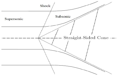
Figure 1. A self-similar transonic shock in three-dimensional steady flow past a straight-sided cone

By scaling the state variables $(u,v,\rho)\to(\tilde{u},\tilde{v},\tilde{\rho})$:

$$(\tilde{u},\tilde{v},\tilde{\rho})=(\frac{u}{u_{\infty}},\frac{v}{u_{\infty}},\frac{\rho}{u_{\infty}^{2/(\gamma-1)}}),$$ (1.4)

the corresponding sound speed becomes $\tilde{c}=\frac{c}{u_{\infty}}$; the equations in (1.1) remain unchanged for the new variables $(\tilde{u},\tilde{v},\tilde{\rho})$, and the Bernoulli constant becomes $\tilde{\kappa}_{\infty}:=\frac{1}{2}+\frac{1}{\gamma-1}\tilde{\rho}_{\infty}^{\gamma-1}$. Therefore, without loss of generality, we can drop “ $\tilde{}\$” for notational convenience hereafter to assume that $u_{\infty}=1$, the Bernoulli constant is

$$\kappa_{\infty}:=\frac{1}{2}+\frac{1}{\gamma-1}\rho_{\infty}^{\gamma-1}.$$ (1.5)

Then we have

$$M_{\infty}^{2}=\rho_{\infty}^{-(\gamma-1)}\quad\text{ or }\quad\nu:=c_{\infty}^{2}=\frac{1}{M_{\infty}^{2}}=\rho_{\infty}^{\gamma-1}.$$ (1.6)

Under this scaling, the problem reduces to the stability problem for self-similar transonic shock-fronts in transonic flow past a perturbed cone, governed by (1.1)–(1.2) with the Bernoulli constant (1.5), when the Mach number $M_{\infty}$ of the upcoming flow is sufficiently large, or equivalently, the density $\rho_{\infty}$ is sufficiently small.

Conical flow (i.e. cylindrically symmetric flow with respect to an axis, say, the $x$-axis) occurs in many physical situations. For instance, it occurs at the conical nose of a projectile facing a supersonic stream of air (cf. [18]). The study of supersonic-supersonic shock-fronts was initiated in Gu [22], Schaeffer [30], and Li [24] first for the wedge case; also see Chen [11, 12, 13], Zhang [34, 35], and Chen-Zhang-Zhu [10] for the recent results. The stability of conical supersonic-supersonic shock-fronts has been studied in the recent years in Liu-Lien [26] in the class of $BV$ solutions when the cone vertex angle is small, and Chen [14] and Chen-Xin-Yin [17] in the class of smooth solutions away from the conical shock-front when the perturbed cone is sufficiently close to the straight-sided cone.

The stability of transonic shock-fronts in three-dimensional steady flow past a perturbed cone has been a longstanding open problem. Some progress has been made for the wedge case in two-dimensional steady flow in Chen-Fang [16] and Fang [19]. In particular, in [16, 19], it was proved that the transonic shock is conditionally stable under perturbation of the upstream flow and/or perturbation of wedge boundary. Also see [5, 6, 7, 15, 31, 32, 33] for steady transonic flow in multidimensional nozzles.

For the two-dimensional wedge case, the equations do not involve singular terms and the flow past the straight-sided wedge is piecewise constant. However, for the three-dimensional conical case, the governing equations have a singularity at the cone vertex and the flow past the straight-sided cone is self-similar, but is no longer piecewise constant. These cause additional difficulties for the stability problem. In this paper, we develop techniques to handle the singular terms in the equations and the singularity of the solutions.

Our main results indicate that the self-similar transonic shock-front is conditionally stable with respect to the conical perturbation of the cone boundary and the upstream flow in appropriate function spaces. That is, it is proved that the transonic shock-front and downstream flow in our solutions are close to the unperturbed self-similar transonic shock-front and downstream flow under the conical perturbation, and the slope of the shock-front asymptotically tends to the slope of the unperturbed self-similar shock at infinity.

In order to achieve these results, we first formulate the stability problem as a free boundary problem and then introduce a coordinate transformation to reduce the free boundary problem into a fixed boundary value problem for a singular nonlinear elliptic system. We develop an iteration scheme that consists of two iteration mappings: one is for an iteration of approximate transonic shock-fronts; and the other is for an iteration of the corresponding boundary value problems for the singular nonlinear systems for given approximate shock-fronts. To ensure the well-definedness and contraction property of the iteration mappings, it is essential to establish the well-posedness for a corresponding singular linearized elliptic equation, especially the stability with respect to the coefficients of the equation, and obtain the estimates of its solutions reflecting their singularity at the cone vertex and decay at infinity. The approach is to employ key features of the equation, introduce appropriate solution spaces, and apply a Fredholm-type theorem in Maz’ya-Plamenevskiǐ [28] to establish the existence of solutions by showing the uniqueness in the solution spaces.

The organization of this paper is as follows. In Section 2, we exploit the behavior of self-similar transonic shocks and corresponding transonic flows past straight-sided cones, governed by (1.1)–(1.2) with Bernoulli constant (1.5). In Section 3, we first formulate the stability problem as a free boundary problem, then introduce a coordinate transformation to reduce the free boundary problem into a fixed boundary value problem, and finally state the main theorem (Theorem 3.1) of this paper and its equivalent theorem (Theorem 3.2).

In Section 4, we establish the well-posedness for a singular linear elliptic equation, which will play an important role for establishing the main theorem, Theorem 3.1. In Section 5, we develop our iteration scheme for the stability problem, which includes two steps: one is an iteration of approximate transonic shock-fronts; and the other is the iteration of the corresponding nonlinear boundary value problems for given approximate shock-fronts. In Sections 6–7, we prove that the two iteration mappings in the iteration scheme are both well-defined, contraction mappings, based on the well-posedness theory for a singular linear elliptic equation established in Section 4. This implies that there exists a unique fixed point of each iteration mapping leading to the completion of the proof of the main theorem, Theorem 3.1.

We remark that all the results for the case $\gamma>1$ is valid for the isothermal case $\gamma=1$ as the limiting case when $\gamma\to 1$, which can be checked step by step in the proofs.

2. Self-similar transonic shocks and corresponding transonic flows past straight-sided cones

In this section, we exploit the behavior of self-similar transonic shocks and corresponding transonic flows past straight-sided cones, governed by (1.1)–(1.2) with Bernoulli constant (1.5).

Let the turning angle of the velocity field right behind the self-similar shock-front $\mathcal{S}$ be $\phi_{1}$ and set $b=\operatorname{tan}\phi_{1}$. Then $v=bu$ for the velocity field $(u,v)$ of the flow right across $\mathcal{S}$. Assume that the angle between $\mathcal{S}$ and the upcoming velocity field $(1,0)$ is $\omega_{1}$ and set $\tau=\operatorname{cot}\omega_{1}$. Then the Rankine-Hugoniot conditions on $\mathcal{S}$ are

$$[\rho u]=\tau[\rho v],\qquad-[v]=\tau[u].$$ (2.1)

Using (2.1) and the relation $v=bu$, we have

$$u=\frac{\tau}{b+\tau},\qquad v=\frac{b\tau}{b+\tau},\qquad\rho=\frac{b+\tau}{\tau(1-b\tau)}\rho_{\infty}.$$ (2.2)

Substitute (2.2) into Bernoulli’s law with Bernoulli constant (1.5) and use $\nu=\frac{1}{M_{\infty}^{2}}$. Then a direct computation yields

$$0=F(\tau,\nu):=\tau-\frac{b+\tau}{1-b\tau}\Big{(}\frac{(\gamma-1)(1+2\tau/b-\tau^{2})}{2(1+\tau/b)^{2}}+\nu\Big{)}^{-\frac{1}{\gamma-1}}\nu^{\frac{1}{\gamma-1}}.$$ (2.3)

For $\gamma>1$ and $b>0$, we have

$$F(0,0)=0,\qquad\partial_{\tau}F(0,0)=1\neq 0.$$

Then the implicit function theorem implies that, in a neighborhood of $(0,0)$, $\tau$ can be expressed as a function of $\nu$, that is, there exists a positive constant $\nu_{0}$ such that

$$\tau=\tau(\nu)\qquad\,\,\mbox{for}\,\,\nu\in[0,\nu_{0}].$$

Furthermore, there exist positive constants $\alpha_{1}$ and $\alpha_{2}$ such that, for any $\nu\in[0,\nu_{0}]$, we have

$$\alpha_{1}\nu^{\frac{1}{\gamma-1}}\leq\tau(\nu)\leq\alpha_{2}\nu^{\frac{1}{\gamma-1}}.$$ (2.4)

By (2.2), we conclude

$$u=O(1)\nu^{\frac{1}{\gamma-1}}\rightarrow 0,\quad v=O(1)\nu^{\frac{1}{\gamma-1}}\rightarrow 0,\quad\rho=O(1)\qquad\,\,\text{ as }\nu\rightarrow 0,$$ (2.5)

where $O(1)$ depends only on $\gamma$ and $b$. Thus,

$$M^{2}=\frac{q^{2}}{\rho^{\gamma-1}}=O(1)\nu^{\frac{2}{\gamma-1}}\rightarrow 0\qquad\text{ as }\,\nu\rightarrow 0,$$ (2.6)

where $q=\sqrt{u^{2}+v^{2}}$ is the flow speed and $O(1)$ depends only on $\gamma$ and $b$.

We now analyze the flow field between the self-similar shock-front $\mathcal{S}$ and the straight-sided cone. Let $\omega_{0}$ be the vertex angle of the cone and $\kappa=\operatorname{cot}\omega_{0}$. Since the equations and the boundary conditions are invariant under the scaling $(x,y)\to(\alpha x,\alpha y),\alpha\neq 0$, we seek self-similar solutions $(u,v)=(u,v)(\sigma),\sigma=\displaystyle x/y$, as in [18]. Then the flow field $(u,v)$ between the shock-front $\mathcal{S}$ and the cone $y=\kappa x$ is determined by the following free boundary value problem:

$$\left\{\begin{aligned} &\partial_{\sigma}v+\sigma\partial_{\sigma}u=0,\\ &\big{(}1-\frac{u^{2}}{c^{2}}\big{)}\partial_{\sigma}u-\big{(}\frac{2uv}{c^{2}}+\sigma(1-\frac{v^{2}}{c^{2}})\big{)}\partial_{\sigma}v+v=0,\end{aligned}\right. \text{ for }\sigma\in(\tau,\kappa),$$ (2.7)

$$(u,v)=\left(u_{S},v_{S}\right), \text{ on }\sigma=\tau,$$ (2.8)

$$u-\kappa v=0, \text{ on }\sigma=\kappa,$$ (2.9)

where $\omega_{0}$ or $\kappa$ is unknown and determined together with the solution, $\tau$ and $(u_{S},v_{S};\rho_{S})$ are determined by the shock polar and the flow direction $b$ right behind the shock-front $\mathcal{S}$ which are given in (2.2), and the density $\rho$ is determined by Bernoulli’s law with Bernoulli constant (1.5).

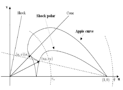
Figure 2. Apple curve and shock polar for the self-similar solutions

By [18], there exists a vertex angle $\omega_{0}=\omega_{0}(b)$ of the cone and the corresponding self-similar solution $(u_{0},v_{0})(\sigma),\ \sigma\in[\tau,k]$, between the shock-front and the cone as the solution of the free boundary value problem (2.7)–(2.9). We assume that the flow between the shock-front and the cone is subsonic, which is the case when $M_{\infty}$ is large (equivalently, $\rho_{\infty}$ is small). In this case, we employ (2.7) to obtain

$$\begin{split}&\Big{(}\big{(}1-\frac{u^{2}}{c^{2}}\big{)}+\frac{2uv}{c^{2}}\sigma+\big{(}1-\frac{v^{2}}{c^{2}})\sigma^{2}\Big{)}\partial_{\sigma}u+v=0,\\ &\Big{(}\big{(}1-\frac{u^{2}}{c^{2}}\big{)}+\frac{2uv}{c^{2}}\sigma+\big{(}1-\frac{v^{2}}{c^{2}})\sigma^{2}\Big{)}\partial_{\sigma}v-\sigma v=0,\\ &\Big{(}\big{(}1-\frac{u^{2}}{c^{2}})+\frac{2uv}{c^{2}}\sigma+\big{(}1-\frac{v^{2}}{c^{2}}\big{)}\sigma^{2}\Big{)}\partial_{\sigma}\big{(}\frac{q^{2}}{2}\big{)}+v(u-\sigma v)=0,\end{split}$$

where $q=\sqrt{u^{2}+v^{2}}$ is the flow speed. It is easy to verify that

$$u_{0}(\sigma)>0,\qquad v_{0}(\sigma)>0,$$

and $u_{0}(\sigma)$, $q_{0}(\sigma)$, and the Mach number $M_{0}(\sigma)$ are strictly decreasing, while $v_{0}(\sigma)$ is strictly increasing, with respect to $\sigma$. Therefore, we have

$$b=\frac{v(\tau)}{u(\tau)}<\frac{v(\kappa)}{u(\kappa)}=\frac{1}{\kappa}=\operatorname{tan}\omega_{0},\quad\text{ i.e.},\,\,\,\,0<\kappa<\frac{1}{b},$$

$$\max\limits_{\sigma\in[\tau,\kappa]}u_{0}(\sigma)=u_{0}(\tau),$$

$$\max\limits_{\sigma\in[\tau,\kappa]}v_{0}(\sigma)=v_{0}(\kappa)<u_{0}(\tau)\operatorname{tan}\omega_{0},$$

$$\max\limits_{\sigma\in[\tau,\kappa]}q_{0}(\sigma)\leq q_{0}(\tau),$$

$$\max\limits_{\sigma\in[\tau,\kappa]}M_{0}(\sigma)\leq M_{0}(\tau)<1.$$

In the next sections, we develop a nonlinear iteration scheme and establish the stability of self-similar transonic shocks under perturbation of the upstream supersonic flow and the boundary surface of the straight-sided cone.

3. Stability Problem and Main Theorem

In this section we first formulate the stability problem as a free boundary value problem, then introduce a coordinate transformation to reduce the free boundary problem into a fixed boundary value problem, and finally state the main theorem (Theorem 3.1) of this paper and its equivalent theorem (Theorem 3.2).

3.1. Formulation of the stability problem

The stability problem can be formulated as the following free boundary problem.

Problem I: Free boundary problem. Determine the free boundary $S=\{x=\phi(y)\}$ and the velocity field $(u,v)$ in the unbounded domain $\{\phi(y)<x<\varphi^{-1}(y)\}$ satisfying the equations:

$$\left\{\begin{aligned} &\partial_{x}(\rho u)+\partial_{y}(\rho v)+\frac{\rho v}{y}=0,\\ &\partial_{x}v-\partial_{y}u=0,\end{aligned}\right.\qquad\qquad\text{ in }\{\phi(y)<x<\varphi^{-1}(y)\},$$ (3.1)

the free boundary conditions on $S$:

$$\quad[\rho u][u]+[\rho v][v]=0,$$ (3.2)

$$\quad-[v]=[u]\phi^{\prime}(y),$$ (3.3)

and the slip boundary condition on the boundary surface of the perturbed cone, $B=\{y=\varphi(x)\}$:

$$v-\varphi^{\prime}(x)\,u=0\qquad\quad\text{ on }B,$$ (3.4)

where the density $\rho$ can be expressed as a function of the velocity $(u,v)$ by Bernoulli’s law:

$$\rho=\rho(q)=\Big{(}\tilde{\kappa}_{\infty}-\frac{\gamma-1}{2}q^{2}\Big{)}^{\frac{1}{\gamma-1}},$$ (3.5)

with $q=\sqrt{u^{2}+v^{2}}$ and $\tilde{\kappa}_{\infty}=(\gamma-1)\kappa_{\infty}$.

The equations in (3.1) can be rewritten in the matrix form:

$$A(U)\partial_{x}U+B(U)\partial_{y}U+C(y)U=0,$$ (3.6)

where $U=(u,v)^{\top}$ and

$$A(U)=\begin{pmatrix}1-\displaystyle\frac{u^{2}}{c^{2}}&-\displaystyle\frac{uv}{c^{2}}\\ 0&1\end{pmatrix},\quad B(U)=\begin{pmatrix}-\displaystyle\frac{uv}{c^{2}}&1-\displaystyle\frac{v^{2}}{c^{2}}\\ -1&0\end{pmatrix},\quad C(y)=\begin{pmatrix}0&\displaystyle\frac{1}{y}\\ 0&0\end{pmatrix}.$$

To solve the free boundary problem (Problem I), we introduce the following coordinate transformation:

$$\Pi_{\phi,\varphi}:\ (x,y)\mapsto(\xi,\eta)$$

to fix the free boundary:

$$\Pi_{\phi,\varphi}:\ \left\{\begin{aligned} &\xi-\eta\operatorname{cot}\omega_{1}=x-\phi(y),\\ &\eta-\xi\operatorname{tan}\omega_{0}=y-\varphi(x).\end{aligned}\right.$$ (3.7)

Then the free boundary $S$ becomes a fixed boundary $\Gamma_{1}=\left\{\xi=\eta\operatorname{cot}\omega_{1}\right\}$, and the domain $\{\phi(y)<x<\varphi^{-1}(y)\}$ becomes a fixed domain

$$\Omega=\left\{\eta\operatorname{cot}\omega_{1}<\xi<\eta\operatorname{cot}\omega_{0}\right\}=\left\{(r,\theta):\ \omega_{0}<\theta<\omega_{1}\right\}.$$

In transformation (3.7), $\phi$ as a function of $y$ is unknown and can be also considered as a function of $\eta$ in the following way:

$$\psi(\eta):=\phi(y(\eta\operatorname{cot}\omega_{1},\eta)).$$

Then the transformation is written as

$$\Pi_{\psi,\varphi}:\ \left\{\begin{aligned} &\xi-\eta\operatorname{cot}\omega_{1}=x-\psi(\eta),\\ &\eta-\xi\operatorname{tan}\omega_{0}=y-\varphi(x).\end{aligned}\right.$$ (3.8)

In the case that $\psi(\eta)$ is known, we can obtain the expression of $\phi(y)$ from (3.8). In fact, substituting $\xi=\eta\operatorname{cot}\omega_{1}$ into (3.8), we have

$$x=\psi(\eta),\qquad y=(1-\operatorname{tan}\omega_{0}\operatorname{cot}\omega_{1})\eta+\varphi\circ\psi(\eta).$$

Thus,

$$\frac{\mathrm{d}y}{\mathrm{d}\eta}=1-\operatorname{tan}\omega_{0}\operatorname{cot}\omega_{1}+\varphi^{\prime}\,\dot{\psi},$$

where $\varphi^{\prime}=\displaystyle\frac{\mathrm{d}\varphi(x)}{\mathrm{d}x}$ and $\dot{\psi}=\displaystyle\frac{\mathrm{d}\psi(\eta)}{\mathrm{d}\eta}$. In our case, $\varphi^{\prime}$ and $\dot{\psi}$ should be small perturbations to $\operatorname{tan}\omega_{0}$ and $\operatorname{cot}\omega_{1}$, respectively. Hence, we have $\displaystyle\frac{\mathrm{d}y}{\mathrm{d}\eta}>0$, and $\eta$ can be also expressed as a function of $y$, i.e. $\eta=\eta(y)$. Then $\phi(y)=\psi(\eta(y))$ is what we need. Therefore, we consider the transformation with formulation (3.8) from now on. Then we have

$$y-\eta=\varphi(x)-\xi\operatorname{tan}\omega_{0}=\big{(}\varphi(x)-x\operatorname{tan}\omega_{0}\big{)}+\operatorname{tan}\omega_{0}\big{(}\psi(\eta)-\eta\operatorname{cot}\omega_{1}\big{)}.$$ (3.9)

A direct calculation indicates that the Jacobian matrix of the transformation is

$$\frac{\partial(\xi,\eta)}{\partial(x,y)}=\frac{1}{1-\operatorname{tan}\omega_{0}(\operatorname{cot}\omega_{1}-\dot{\psi})}\begin{pmatrix}1-\varphi^{\prime}(x)(\operatorname{cot}\omega_{1}-\dot{\psi})&\operatorname{cot}\omega_{1}-\dot{\psi}\\ \operatorname{tan}\omega_{0}-\varphi^{\prime}(x)&1\end{pmatrix},$$ (3.10)

or

$$\frac{\partial(x,y)}{\partial(\xi,\eta)}=\begin{pmatrix}1&\dot{\psi}-\operatorname{cot}\omega_{1}\\ \varphi^{\prime}(x)-\operatorname{tan}\omega_{0}&1+\varphi^{\prime}(x)(\dot{\psi}-\operatorname{cot}\omega_{1})\end{pmatrix}.$$ (3.11)

Then, under the transformation, system (3.6) becomes

$$A(U)\partial_{\xi}U+B(U)\partial_{\eta}U+C(\eta)U=\mathscr{F}(U;\psi)\qquad\text{ in }\Omega,$$ (3.12)

where

$$C(\eta)=\begin{pmatrix}0&\displaystyle{1}/{\eta}\\ 0&0\end{pmatrix},$$

and

$$\mathscr{F}(U;\psi)=\tilde{C}(\eta;\psi)U-\tilde{A}(U;\psi)D_{2}U-\tilde{B}(U;\psi)D_{1}U,$$

and

$$\tilde{A}(U;\psi):=\frac{\operatorname{tan}\omega_{0}-\varphi^{\prime}}{1-\operatorname{tan}\omega_{0}(\operatorname{cot}\omega_{1}-\dot{\psi})}A(U),$$

$$\tilde{B}(U;\psi):=\frac{\operatorname{cot}\omega_{1}-\dot{\psi}}{1-\operatorname{tan}\omega_{0}(\operatorname{cot}\omega_{1}-\dot{\psi})}B(U),$$

$$\tilde{C}(\eta;\psi):=\begin{pmatrix}0&\displaystyle\frac{1}{\eta}-\frac{1}{y(\eta;\psi)}\\ 0&0\end{pmatrix},$$

$$(D_{1},D_{2}):=(\partial_{\xi}+\operatorname{tan}\omega_{0}\,\partial_{\eta},(\operatorname{cot}\omega_{1}-\dot{\psi})\,\partial_{\xi}+\partial_{\eta}).$$

Since $\psi(\eta)=\phi(y(\eta\operatorname{cot}\omega_{1},\eta))$, we have

$$\dot{\psi}=(\partial_{\xi}y\operatorname{cot}\omega_{1}+\partial_{\eta}y)\phi^{\prime}=(1-\operatorname{tan}\omega_{0}\operatorname{cot}\omega_{1}+\varphi^{\prime}\,\dot{\psi})\phi^{\prime},$$

and the boundary condition (3.3) becomes

$$\dot{\psi}=\frac{1-\operatorname{tan}\omega_{0}\operatorname{cot}\omega_{1}}{1-\varphi^{\prime}(x)\phi^{\prime}(y)}\phi^{\prime}(y)=-\frac{[v](1-\operatorname{tan}\omega_{0}\operatorname{cot}\omega_{1})}{[u]+\varphi^{\prime}(x)\,[v]}.$$ (3.13)

With these, the free boundary problem (3.1)—(3.4) becomes the following fixed boundary problem:

Problem II: Fixed boundary problem. Determine the functions $(U;\psi)=(u,v;\psi)$ in the unbounded domain:

$$\Omega:=\left\{\eta\operatorname{cot}\omega_{1}<\xi<\eta\operatorname{cot}\omega_{0}\right\}=\left\{(r,\theta):\ \omega_{0}<\theta<\omega_{1}\right\}$$

satisfying system (3.12) and the boundary conditions: (3.2) and (3.13) on $\Gamma_{1}:=\{\xi=\eta\operatorname{cot}\omega_{1}\}$ and (3.4) on $\Gamma_{0}:=\{\xi=\eta\operatorname{cot}\omega_{0}\}$.

3.2. Weighted spaces for solutions

Based on the analysis of the self-similar transonic shock solutions in Section 2 and the behavior of solutions to elliptic equations at infinity, it is anticipated that the solutions have singularity at the origin and decay at infinity. Thus, we need the following weighted spaces as posed spaces to accommodate the features of solutions to our problem.

Let $1<q<\infty$ and $0\leq\omega_{0}<\omega_{1}\leq 2\pi$. Let

$$\mathscr{D}:=\left\{x\in\mathbb{R}^{2}:\ 0<r<\infty,\omega_{0}<\theta<\omega_{1}\right\}$$

be an unbounded sector, where $(r,\theta)$ are the polar coordinates. Then the boundary of the domain $\mathscr{D}$ consists of two rays:

$$\Gamma_{0}:=\left\{x\in\mathbb{R}^{2}:\ \theta=\omega_{0},0<r<\infty\right\},\qquad\Gamma_{1}=\left\{x\in\mathbb{R}^{2}:\ \theta=\omega_{1},0<r<\infty\right\}.$$

For any $k\in\mathbb{R}$, $m=0,1,\cdots$, we define the following weighted Sobolev spaces $W^{m,q}_{(k)}(\mathscr{D})$ as subspaces of $u\in W^{m,q}_{loc}(\mathscr{D})$:

$$W^{m,q}_{(k)}(\mathscr{D})=\left\{u\in W_{loc}^{m,q}(\mathscr{D}):\ \left\|u\right\|_{W_{(k)}^{m,q}(\mathscr{D})}<\infty\right\},$$

with the norms:

$$\left\|u(r,\theta)\right\|_{W_{(k)}^{m,q}(\mathscr{D})}=\left\|\mathrm{e}^{kt}u(\mathrm{e}^{t},\theta)\right\|_{W^{m,q}(\mathcal{P}(\mathscr{D}))},$$ (3.14)

where

$$\mathcal{P}(r,\theta)=(t,\theta):=(\ln r,\theta)$$ (3.15)

is a coordinate transformation from $(r,\theta)$ to $(t,\theta)$.

Define the norms for the trace of $u$ on each ray $\Gamma_{j}$ of the boundary of $\mathscr{D}$ by

$$\left\|u(r,\omega_{j})\right\|_{W^{m-1/q,q}_{(k)}(\Gamma_{j})}=\left\|\mathrm{e}^{tk}u\left(t,\omega_{j}\right)\right\|_{W^{m-1/q,q}(\mathbb{R})},\qquad j=0,1.$$ (3.16)

It is easy to see that there exists a constant $K$, independent of $u$, such that

$$\left\|u\right\|_{W^{m-{1}/{q},q}_{(k)}(\Gamma_{j})}\leq K\,\left\|u\right\|_{W^{m,q}_{(k)}(\mathscr{D})}.$$

Define

$$\left\|u(r,\theta)\right\|_{C^{m}_{(k)}(\mathscr{D})}=\left\|\mathrm{e}^{kt}u(\mathrm{e}^{t},\theta)\right\|_{C^{m}(\mathcal{P}(\mathscr{D}))},$$ (3.17)

and denote by $C^{m}_{(k)}(\mathscr{D})$ the space of functions with norm $\left\|\cdot\right\|_{C^{m}_{(k)}(\mathscr{D})}$.

When $q>2$ and $m\geq 1$, the well-known Sobolev imbedding theorem implies that $W^{m,q}_{(k)}(\mathscr{D})$ is embedded in $C^{m-1}_{(k)}(\mathscr{D})$, i.e., there exists a constant $K$, independent of $u$, such that

$$\left\|u\right\|_{C^{m-1}_{(k)}(\mathscr{D})}\leq K\,\left\|u\right\|_{W^{m,q}_{(k)}(\mathscr{D})}.$$ (3.18)

For functions of single variable defined in $\mathbb{R}_{+}$, we can also define the following similar weighted norms:

$$\left\|u(r)\right\|_{W_{(k)}^{m,q}(\mathbb{R}_{+})}=\left\|\mathrm{e}^{kt}u(\mathrm{e}^{t})\right\|_{W^{m,q}(\mathbb{R})},\,\,\,\left\|u(r)\right\|_{C^{m}_{(k)}(\mathbb{R}_{+})}=\left\|\mathrm{e}^{kt}u(\mathrm{e}^{t})\right\|_{C^{m}(\mathbb{R})}.$$ (3.19)

3.3. Main Theorem

The main theorem of this paper is the following.

Theorem 3.1 (Main theorem).

Let $q>2$, $1<\gamma\leq 2$, and $b>0$. Let

$$\{(1,0;\rho_{\infty});(u_{0},v_{0})(\sigma);\phi_{1}=y\operatorname{cot}\omega_{1}\},$$

with $\sigma\in[\operatorname{cot}\omega_{1},\operatorname{cot}\omega_{0}]$ and $b=\frac{v_{0}(\operatorname{cot}\omega_{1})}{u_{0}(\operatorname{cot}\omega_{1})}$, form a transonic shock solution to (3.1) when the upstream flow $(1,0;\rho_{\infty})$ past the straight-sided cone with $y=\varphi_{0}(x)=x\operatorname{tan}\omega_{0}$. Then there exist positive constants $\nu_{0}$, $\varepsilon_{0}$, $M$, and $M_{S}$ ($M$ and $M_{S}$ are independent of $\nu_{0}$ and $\varepsilon_{0}$) such that, if the Mach number $M_{\infty}$ is sufficiently large so that $\nu:=\rho_{\infty}^{\gamma-1}=1/M_{\infty}^{2}\leq\nu_{0}$, then, for any $0<\varepsilon\leq\varepsilon_{0}$ and $\varepsilon\ll\nu^{\frac{1}{\gamma-1}}$, there exists a unique solution $(U(\xi,\eta);\psi(\eta))$ to the fixed boundary value problem (3.12), (3.2), (3.13), and (3.4) satisfying $\psi(0)=0$ and the following estimates:

$$\left\|U-U_{0}\right\|_{W^{1,q}_{(0)}(\Omega)}\leq M\varepsilon,$$ (3.20)

$$\|\dot{\psi}-\operatorname{cot}\omega_{1}\|_{\Gamma_{1}}\leq M_{S}\varepsilon,$$ (3.21)

with $\left\|\cdot\right\|_{\Gamma_{1}}:=\left\|\cdot\right\|_{W_{(0)}^{0,q}(\Gamma_{1})}+\left\|\cdot\right\|_{C^{0}(\Gamma_{1})}$, provided that, if the perturbed boundary $y=\varphi(x)$ of the cone satisfies $\varphi(0)=0$ and

$$\left\|\varphi^{\prime}(x)-\operatorname{tan}\omega_{0}\right\|_{C^{2}_{(0)}(\mathbb{R}_{+})}+\left\|\varphi^{\prime}(x)-\operatorname{tan}\omega_{0}\right\|_{W^{1,q}_{(0)}(\mathbb{R}_{+})}\leq\varepsilon,$$ (3.22)

and the perturbed upstream flow field $U^{-}$ satisfies

$$\left\|U^{-}\right\|_{W^{1,q}_{(0)}(\Omega_{e})}+\left\|\partial_{\xi}U^{-}\right\|_{C^{1}_{(1)}(\Omega_{e})}\leq\varepsilon,$$ (3.23)

where $\Omega_{e}:=\{\eta\cot(\omega_{1}+\hat{\delta}_{0})<\xi<\eta\cot(\omega_{0}-\hat{\delta}_{0})\}$ for some small $\hat{\delta}_{0}>0$,

Since $\Pi_{\psi,\varphi}$ or $\Pi_{\phi,\varphi}$ is invertible, we conclude the following equivalent result from Theorem 3.1.

Theorem 3.2.

Suppose that the assumptions of Theorem 3.1 hold. Then there exist positive constants $\nu_{0}$, $\varepsilon_{0}$, $M$, and $M_{S}$ ($M$ and $M_{S}$ are independent of $\nu_{0}$ and $\varepsilon_{0}$) such that, if the Mach number $M_{\infty}$ is sufficiently large so that $\nu:=\rho_{\infty}^{\gamma-1}=1/M_{\infty}^{2}\leq\nu_{0}$, then, for any $0<\varepsilon\leq\varepsilon_{0}$ and $\varepsilon\ll\nu^{\frac{1}{\gamma-1}}$, there exists a unique solution (still denoted by) $(U(x,y);\phi(y))$ to the free boundary problem (3.1)–(3.4), provided that, if the boundary surface $y=\varphi(x)$ of the perturbed cone satisfies $\varphi(0)=0$ and

$$\left\|\varphi^{\prime}(x)-\operatorname{tan}\omega_{0}\right\|_{C^{2}_{(0)}(\mathbb{R}_{+})}+\left\|\varphi^{\prime}(x)-\operatorname{tan}\omega_{0}\right\|_{W^{1,q}_{(0)}(\mathbb{R}_{+})}\leq\varepsilon,$$ (3.24)

and the perturbed upstream flow field $U^{-}$ satisfies

$$\left\|U^{-}\right\|_{W^{1,q}_{(0)}(\Omega_{e})}+\left\|\nabla U^{-}\right\|_{C^{1}_{(1)}(\Omega_{e})}\leq\varepsilon,$$ (3.25)

where $\Omega_{e}:=\{y\cot(\omega_{1}+\delta_{0})<x<y\cot(\omega_{0}-\delta_{0})\}$ for some small $\delta_{0}>0$. Moreover, the solution $(U(x,y);\phi(y))$ satisfies $\phi(0)=0$ and the following estimates:

$$\left\|U\circ\Pi_{\phi,\varphi}^{-1}-U_{0}\circ\Pi_{\phi_{0},\varphi_{0}}^{-1}\right\|_{W^{1,q}_{(0)}(\Omega)}\leq M\varepsilon,$$ (3.26)

$$\left\|\phi^{\prime}-\operatorname{cot}\omega_{1}\right\|_{S}\leq M_{S}\varepsilon,$$ (3.27)

where $\phi^{\prime}=\frac{\mathrm{d}\phi}{\mathrm{d}y}$ and $\left\|\cdot\right\|_{S}:=\left\|\cdot\right\|_{W_{(0)}^{0,q}(\mathbb{R}_{+})}+\left\|\cdot\right\|_{C^{0}(\mathbb{R}_{+})}$.

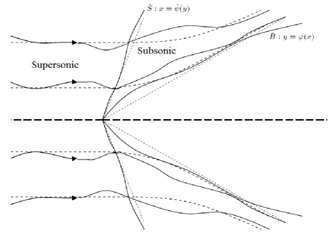
Figure 3. Stability of transonic shock-front solutions

Remark 3.1.

The existence of the perturbed upstream flow field $U^{-}$ satisfying (3.25) can be obtained by blowing up the angular point and then following the standard argument as in Li-Yu [25], since the equations are still quasilinear hyperbolic under the transformation.

Remark 3.2.

Estimates (3.26) and (3.27) imply that the downstream flow and the transonic shock-front are a perturbation of the self-similar transonic shock solution. Hence, the self-similar transonic shock-front is conditionally stable with respect to the conical perturbation of the boundary surface of the cone and the upstream flow in the function spaces with restrictions on the downstream flow field both at the corner and at infinity.

4. Well-posedness for a Singular Linear Elliptic Problem

In this section, we establish the well-posedness for a singular linear elliptic equation, which will play an essential role for establishing the main theorem, Theorem 3.1.

Let $0<\omega_{0}<\omega_{1}<\frac{\pi}{2}$ and set

$$\begin{split}&\Omega:=\left\{(x,y)\in\mathbb{R}^{2}:\ 0<r<\infty,\omega_{0}<\theta<\omega_{1}\right\},\\ &\Gamma_{0}:=\left\{(x,y)\in\mathbb{R}^{2}:\ 0<r<\infty,\theta=\omega_{0}\right\},\\ &\Gamma_{1}:=\left\{(x,y)\in\mathbb{R}^{2}:\ 0<r<\infty,\theta=\omega_{1}\right\},\end{split}$$

where $(r,\theta)$ are the polar coordinates in the plane.

4.1. Neumann problem for a singular second-order elliptic equation

Consider the following Neumann boundary value problem in $\Omega$:

$$\left\{\begin{aligned} &L_{0}\varphi:=\partial_{xx}\varphi+\partial_{yy}\varphi+\frac{\partial_{y}\varphi}{y}=f\quad&\text{ in }\Omega,\\ &B_{0}\varphi:=\partial_{y}\varphi-\operatorname{tan}\omega_{0}\partial_{x}\varphi=g_{0}&\text{ on }\Gamma_{0},\\ &B_{1}\varphi:=\partial_{x}\varphi-\operatorname{cot}\omega_{1}\partial_{y}\varphi=g_{1}&\text{ on }\Gamma_{1}.\end{aligned}\right.$$ (4.1)

We have the following proposition.

Proposition 4.1.

Let $1<q<\infty$. The operator $(L_{0},B_{0},B_{1})$ defined in (4.1) realizes an isomorphism from $W_{(-1)}^{2,q}(\Omega)$ to $W_{(1)}^{0,q}(\Omega)\times(W_{(0)}^{1-1/q,q}(\mathbb{R}_{+}))^{2}$. Moreover, we have the following estimate for the solution to problem (4.1):

$$\left\|\varphi\right\|_{W_{(-1)}^{2,q}(\Omega)}\leq K\,\Big{(}\left\|f\right\|_{W_{(1)}^{0,q}(\Omega)}+\sum_{j=0,1}\left\|g_{j}\right\|_{W_{(0)}^{1-1/q,q}(\mathbb{R}_{+})}\Big{)},$$ (4.2)

where the constant $K$ is independent of $\varphi$, but depends only on $q$ and $\omega_{0}$ (actually $\operatorname{cot}\omega_{0}$).

To prove this proposition, we employ a criterion identified by Hartman-Wintner [23] for the uniqueness of solutions to the Dirichlet boundary value problem for systems of second-order differential equations. For self-containedness, we give a brief description here; for more details, see [23].

Lemma 4.1.

Consider the following boundary value problem for the system of second-order differential equations for $x\in\mathbb{R}^{n}$:

$$\left\{\begin{aligned} &x^{\prime\prime}+A_{1}(t)\,x^{\prime}+A_{2}(t)\,x=0\qquad\text{for}\,\,t\in(t_{0},t_{1}),\\ &x(t_{0})=x(t_{1})=0,\end{aligned}\right.$$ (4.3)

where $A_{1}(t)$ and $A_{2}(t)$ are $n\times n$ real matrices. Assume that there exists a matrix $K(t)$ such that

$$N=(K^{0})^{\prime}-A_{2}^{0}-\big{(}\frac{1}{2}A_{1}-K^{0}\big{)}\big{(}\frac{1}{2}A_{1}^{\top}-K^{0})>0,$$ (4.4)

where $K^{0}=\frac{1}{2}(K+K^{\top})$ and $A_{2}^{0}=\frac{1}{2}(A_{2}+A_{2}^{\top})$. Then problem (4.3) has only the trivial solution $x\equiv 0$.

Proof.

Taking the inner product on the equations with $x$ and integrating from $t_{0}$ to $t_{1}$ yields

$$\int_{t_{0}}^{t_{1}}\left(x^{\prime}\cdot x^{\prime}-x\cdot A_{1}x^{\prime}-x\cdot A_{2}x\right)\mathrm{d}t=0.$$ (4.5)

Since $(x\cdot Kx)^{\prime}=2x^{\prime}\cdot K^{0}x+x\cdot K^{\prime}x$, we have

$$0=\int_{t_{0}}^{t_{1}}(x\cdot Kx)^{\prime}\mathrm{d}t=\int_{t_{0}}^{t_{1}}(2x^{\prime}\cdot K^{0}x+x\cdot K^{\prime}x)\,\mathrm{d}t.$$ (4.6)

Then

$$\int_{t_{0}}^{t_{1}}\Big{(}\big{|}x^{\prime}-\big{(}\frac{1}{2}A_{1}^{\top}-K^{0}\big{)}x\big{|}^{2}+x\cdot Lx\Big{)}\mathrm{d}t=0,$$

where $L:=K^{\prime}-A_{2}-\big{(}\frac{1}{2}A_{1}-K^{0}\big{)}\big{(}\frac{1}{2}A_{1}^{\top}-K^{0})$.

Similarly, we have

$$\int_{t_{0}}^{t_{1}}\Big{(}\big{|}x^{\prime}-\big{(}\frac{1}{2}A_{1}^{\top}-K^{0}\big{)}x\big{|}^{2}+x\cdot L^{\top}x\Big{)}\mathrm{d}t=0.$$

Combining the above two identities, we obtain

$$\int_{t_{0}}^{t_{1}}\Big{(}\big{|}x^{\prime}-\big{(}\frac{1}{2}A_{1}^{\top}-K^{0}\big{)}x\big{|}^{2}+x\cdot Nx\Big{)}\mathrm{d}t=0.$$

Since $N$ is positive definite, we conclude $x\equiv 0$. ∎

Proof of Proposition 4.1.

Rewriting the boundary value problem (4.1) in the polar coordinates $(r,\theta)$, we have

$$\left\{\begin{aligned} &L_{0}\varphi=(r\partial_{r})^{2}\varphi+\partial_{\theta}^{2}\varphi+r\partial_{r}\varphi+\operatorname{cot}\theta\,\partial_{\theta}\varphi=r^{2}f&\text{in }\Omega,\\ &B_{0}\varphi=\partial_{\theta}\varphi=rg_{0}&\text{ on }\Gamma_{0},\\ &B_{1}\varphi=\partial_{\theta}\varphi=rg_{1}&\text{ on }\Gamma_{1}.\end{aligned}\right.$$ (4.7)

Employing the transformation $\mathcal{P}$ in (3.15), i.e., $\mathcal{P}(r,\theta)=(t,\theta)=(\ln r,\theta)$, we convert the infinite sector $\Omega$ into an infinite strip: $\mathscr{D}:=\left\{(t,\theta):\ t\in\mathbb{R},\ \omega_{0}<\theta<\omega_{1}\right\}$. Accordingly, the boundary value problem (4.7) is converted to the following boundary value problem in $\mathscr{D}$:

$$\left\{\begin{aligned} &\partial_{tt}\varphi+\partial_{\theta\theta}\varphi+\partial_{t}\varphi+\operatorname{cot}\theta\,\partial_{\theta}\varphi=\mathrm{e}^{2t}f&\text{ in }\mathscr{D},\\ &\partial_{\theta}\varphi=\mathrm{e}^{t}g_{0}&\text{ on }\Sigma_{0},\\ &\partial_{\theta}\varphi=\mathrm{e}^{t}g_{1}&\text{ on }\Sigma_{1}.\end{aligned}\right.$$ (4.8)

Applying the Fourier transformation $\mathscr{F}_{t\rightarrow\lambda}$ with respect to $t$, we obtain a family of boundary value problems with complex parameter $\lambda$:

$$\left\{\begin{aligned} &\hat{\varphi}^{\prime\prime}+\operatorname{cot}\theta\,\hat{\varphi}^{\prime}+(-\lambda^{2}+\mathrm{i}\lambda)\varphi=\widehat{\mathrm{e}^{2t}f}\qquad&\theta\in(\omega_{0},\omega_{1}),\\ &\hat{\varphi}^{\prime}=\widehat{\mathrm{e}^{t}g_{0}}\qquad&\theta=\omega_{0},\\ &\hat{\varphi}^{\prime}=\widehat{\mathrm{e}^{t}g_{1}}\qquad&\theta=\omega_{1}.\end{aligned}\right.$$ (4.9)

We now employ a Fredholm-type theorem, Theorem A.1 in Appendix, to find that, if the homogeneous problems of (4.9) (i.e. $f=g_{0}=g_{1}=0$) have only the trivial solution $\hat{\varphi}\equiv 0$ for all $\lambda$ with $\text{Im}\lambda=-1$, then, for any $(f,g_{0},g_{1})$ such that $\mathrm{e}^{t}f\in W^{0,q}(\mathscr{D})$ and $g_{j}\in W^{1-1/q,q}(\Sigma_{j}),j=0,1$, the boundary value problem (4.8) in the infinite strip $\mathscr{D}$ has a unique solution $\varphi$ such that $\mathrm{e}^{-t}\varphi\in W^{2,q}(\mathscr{D})$. Moreover, the solution $\varphi$ satisfies the estimate:

$$\left\|\mathrm{e}^{-t}\varphi\right\|_{W^{2,q}(\mathscr{D})}\leq K\,\Big{(}\left\|\mathrm{e}^{t}f\right\|_{W^{0,q}(\mathscr{D})}+\sum_{j=0,1}\left\|g_{j}\right\|_{W^{1-1/q,q}(\Sigma_{j})}\Big{)},$$ (4.10)

where $K$ is independent of $\varphi$, but does depend on $\omega_{0}$ because of the coefficient $\operatorname{cot}\theta$. Then the results of Proposition 4.1 follow. Therefore, it suffices to verify that, in the case that $f=g_{1}=g_{2}\equiv 0$, the boundary value problems (4.9) with complex parameter $\lambda$, $\text{Im}\lambda=-1$, have only the trivial solution $\hat{\varphi}\equiv 0$.

When $f=g_{0}=g_{1}\equiv 0$, we set $y=\hat{\varphi}^{\prime}$ to have

$$\left\{\begin{aligned} &y^{\prime\prime}+\operatorname{cot}\theta\ y^{\prime}+(-\csc^{2}\theta-\lambda^{2}+\mathrm{i}\lambda)\,\varphi=0\qquad&\text{for }\,\theta\in(\omega_{0},\omega_{1}),\\ &y=0&\text{for}\,\,\theta=\omega_{0},\\ &y=0&\text{for}\,\,\theta=\omega_{1}.\end{aligned}\right.$$ (4.11)

Write $y=y_{1}+y_{2}\mathrm{i}$ and $\lambda=\mu-\mathrm{i}$. Then $-\lambda^{2}+\lambda\mathrm{i}=-\mu^{2}+2+3\mu\mathrm{i}$, and (4.11) can be rewritten as the following boundary value problems of second-order differential equations with real coefficients:

$$\left\{\begin{aligned} &\begin{aligned} &\begin{pmatrix}y_{1}\\ y_{2}\end{pmatrix}^{\prime\prime}+\begin{pmatrix}\operatorname{cot}\theta&0\\ 0&\operatorname{cot}\theta\end{pmatrix}\begin{pmatrix}y_{1}\\ y_{2}\end{pmatrix}^{\prime}\\ &\quad+\begin{pmatrix}-\csc^{2}\theta-\mu^{2}+2&-3\mu\\ 3\mu&-\csc^{2}\theta-\mu^{2}+2\end{pmatrix}\begin{pmatrix}y_{1}\\ y_{2}\end{pmatrix}=0\qquad\,\,\text{for}\,\,\theta\in(\omega_{0},\omega_{1}),\end{aligned}\\ &\begin{pmatrix}y_{1}\\ y_{2}\end{pmatrix}=0\qquad\quad\qquad\qquad\qquad\qquad\qquad\qquad\qquad\qquad\qquad\quad\text{on}\,\,\theta=\omega_{0},\omega_{1}.\end{aligned}\right.$$ (4.12)

Let $K(\theta)=K^{0}(\theta)=\begin{pmatrix}\operatorname{tan}\theta&0\\ 0&\operatorname{tan}\theta\end{pmatrix}$. Then

$$N=\begin{pmatrix}a(\theta,\mu)&0\\ 0&a(\theta,\mu)\end{pmatrix},$$

where

$$\begin{split}a(\theta,\mu):=&(\operatorname{tan}\theta)^{\prime}-(-\csc^{2}\theta-\mu^{2}+2)-(\frac{1}{2}\operatorname{cot}\theta-\kappa)^{2}\\ =&\mu^{2}+\csc^{2}\theta-\frac{1}{4}\operatorname{cot}^{2}\theta>0,\\ \end{split}$$

which implies that the symmetric matrix $N$ is positive definite and hence satisfies the criterion (4.4). By Lemma 4.1, we obtain that $y\equiv 0$. That is, $\hat{\varphi}\equiv const.$ Then the equations in (4.9) yields that $\hat{\varphi}\equiv 0$ for any $\text{Im}\lambda=-1$. This completes the proof. ∎

Proposition 4.1 can be directly applied to a special boundary value problem of first-order partial differential equations.

4.2. A boundary value problem of a singular first-order elliptic system

Consider the boundary value problem for the first-order system:

$$\hat{A}\,\partial_{x}U+\hat{B}\,\partial_{y}U+\hat{C}\,U=F \text{ in }\Omega,$$ (4.13)

$$U\cdot\hat{\alpha}_{0}=g_{0} \text{ on }\Gamma_{0},$$ (4.14)

$$U\cdot\hat{\alpha}_{1}=g_{1} \text{ on }\Gamma_{1},$$ (4.15)

where $U=(u,v)^{\top}$, $\hat{\alpha}_{0}=(-\operatorname{tan}\omega_{0},1)^{\top}$, $\hat{\alpha}_{1}=(1,-\operatorname{cot}\omega_{1})^{\top}$, $F=(f_{1},f_{2})^{\top}$, and

$$\hat{A}=\begin{pmatrix}1&0\\ 0&1\end{pmatrix},\qquad\hat{B}=\begin{pmatrix}0&1\\ -1&0\end{pmatrix},\qquad\hat{C}=\begin{pmatrix}0&\frac{1}{y}\\ 0&0\end{pmatrix}.$$ (4.16)

To solve this problem, we first construct a function $\Phi\in W^{2,q}_{(-1)}(\Omega)$ such that

$$\left\{\begin{aligned} &\triangle\Phi=f_{2}&\text{ in }\Omega,\\ &\Phi=0&\text{ on }\Gamma_{0},\\ &\Phi=0&\text{ on }\Gamma_{1}.\end{aligned}\right.$$ (4.17)

By virtue of [28], there exists a unique $\Phi$ with the following estimate:

$$\left\|\Phi\right\|_{W^{2,q}_{(-1)}(\Omega)}\leq K\,\left\|f_{2}\right\|_{W^{0,q}_{(1)}(\Omega)},$$ (4.18)

where $K$ is independent of $\Phi$.

Let $\tilde{u}=u+\partial_{y}\Phi$ and $\tilde{v}=v-\partial_{x}\Phi$. Then the boundary value problem (4.13)—(4.15) is reduced to

$$\hat{A}\,\partial_{x}\tilde{U}+\hat{B}\,\partial_{y}\tilde{U}+\hat{C}\,\tilde{U}=\tilde{F} \text{ in }\Omega,$$ (4.19)

$$\tilde{U}\cdot\hat{\alpha}_{0}=\tilde{g}_{0} \text{ on }\Gamma_{0},$$ (4.20)

$$\tilde{U}\cdot\bar{\alpha}_{1}=\tilde{g}_{1} \text{ on }\Gamma_{1},$$ (4.21)

where $\tilde{F}=(\tilde{f},0)^{\top}$, $\tilde{f}=f_{1}-\displaystyle\frac{\partial_{x}\Phi}{y}$, $\tilde{g}_{0}=g_{0}$, and $\tilde{g}_{1}=g_{1}$. Since

$$\begin{split}\left\|\frac{\partial_{x}\Phi}{y}\right\|_{W_{(1)}^{0,q}(\Omega)}=&\left\|\mathrm{e}^{t}\,\frac{\partial_{x}\Phi(\mathrm{e}^{t},\theta)}{\mathrm{e}^{t}\sin\theta}\right\|_{W^{0,q}(\mathcal{P}(\Omega))}\leq K(\omega_{0})\left\|\partial_{x}\Phi(\mathrm{e}^{t},\theta)\right\|_{W^{0,q}(\mathcal{P}(\Omega))}\\ =&K(\omega_{0})\left\|\partial_{x}\Phi\right\|_{W_{(0)}^{0,q}(\Omega)}\leq K(\omega_{0})\left\|f_{2}\right\|_{W_{(1)}^{0,q}(\Omega)},\end{split}$$

we have

$$\left\|\tilde{f}\right\|_{W_{(1)}^{0,q}(\Omega)}\leq K(\omega_{0})\sum_{j=1,2}\left\|f_{j}\right\|_{W_{(1)}^{0,q}(\Omega)}=C(\omega_{0})\left\|F\right\|_{W_{(1)}^{0,q}(\Omega)}.$$

By the second equation of (4.19), there exists a potential function $\varphi$ such that $\nabla\varphi=(\partial_{x}\varphi,\partial_{y}\varphi)=\tilde{U}$. Then the boundary value problem (4.19)—(4.21) can be reformulated as a boundary value problem of a second-order elliptic equation:

$$\left\{\begin{aligned} &\partial_{xx}\varphi+\partial_{yy}\varphi+\frac{\partial_{y}\varphi}{y}=\tilde{f}&\text{ in }\Omega,\\ &\partial_{y}\varphi-\operatorname{tan}\omega_{0}\partial_{x}\varphi=\tilde{g}_{0}&\text{ on }\Gamma_{0},\\ &\partial_{x}\varphi-\operatorname{cot}\omega_{1}\partial_{y}\varphi=\tilde{g}_{1}&\text{ on }\Gamma_{1}.\end{aligned}\right.$$

Now Proposition 4.1 yields that there exists a unique solution $\varphi\in W_{(-1)}^{2,q}(\Omega)$ with the following estimate:

$$\begin{split}\left\|\varphi\right\|_{W_{(-1)}^{2,q}(\Omega)}\leq&\,K\,\Big{(}\|\tilde{f}\|_{W_{(1)}^{0,q}(\Omega)}+\sum_{j=0,1}\left\|\tilde{g_{j}}\right\|_{W_{(0)}^{1-1/q,q}(\Gamma_{j})}\Big{)}\\ \leq&\,K\,\Big{(}\left\|F\right\|_{W_{(1)}^{0,q}(\Omega)}+\sum_{j=0,1}\left\|g_{j}\right\|_{W_{(0)}^{1-1/q,q}(\Gamma_{j})}\Big{)},\end{split}$$ (4.22)

where $K$ depends only on $\omega_{0}$, but is independent of $\varphi$, $F$, and $g_{j},j=0,1$. Thus, there exists a unique solution $U\in(W_{(0)}^{1,q}(\Omega))^{2}$ to problem (4.13)—(4.15) with the following estimate:

$$\left\|U\right\|_{W_{(0)}^{1,q}(\Omega)}\leq\hat{K}\,\Big{(}\left\|F\right\|_{W_{(1)}^{0,q}(\Omega)}+\sum_{j=0,1}\left\|g_{j}\right\|_{W_{(0)}^{1-1/q,q}(\Gamma_{j})}\Big{)},$$ (4.23)

where $\hat{K}$ is independent of $U$, $F$, and $g_{j},j=0,1$, but depends only on $\omega_{0}$.

With the argument above, we obtain the following corollary of Proposition 4.1:

Proposition 4.2.

Let $1<q<\infty$. Let $F\in(W_{(1)}^{0,q}(\Omega))^{2}$ and $g_{j}\in W_{(0)}^{1-1/q,q}(\Gamma_{j})$, $j=0,1$. Then there exists a unique solution $U\in(W_{(0)}^{1,q}(\Omega))^{2}$ to the boundary value problem (4.13)—(4.15). Moreover, the solution satisfies estimate (4.23).

Applying the continuity method, we can extend this result to a small “perturbed” boundary value problem for the first-order elliptic system.

4.3. A small perturbed boundary value problem for a singular first-order elliptic system

Consider the following boundary value problem:

$$A\,\partial_{x}U+B\,\partial_{y}U+C\,U=F \text{ in }\Omega,$$ (4.24)

$$U\cdot\alpha_{0}=g_{0} \text{ on }\Gamma_{0},$$ (4.25)

$$U\cdot\alpha_{1}=g_{1} \text{ on }\Gamma_{1},$$ (4.26)

where $A$, $B$, and $C$ are $2\times 2$ matrix functions defined on $\Omega$, $\alpha_{j}=(\alpha_{j1},\alpha_{j2})^{\top}$ are vector functions defined on $\Gamma_{j}$, $j=0,1$. Then we have

Proposition 4.3.

There exists a positive constant $\hat{\epsilon}$, depending only on the constant $\hat{K}$ on the right side of estimate (4.23), such that, if the coefficients of problem (4.24)—(4.26) satisfy the following conditions:

$$\left\|(A-\hat{A},B-\hat{B})\right\|_{C^{0}(\Omega)}+\left\|C-\hat{C}\right\|_{C^{0}_{(1)}(\Omega)}+\sum_{j=0,1}\left\|\alpha_{j}-\hat{\alpha}_{j}\right\|_{C^{1}_{(0)}(\Gamma_{j})}\leq\hat{\epsilon},$$ (4.27)

then, for any $F\in(W_{(1)}^{0,q}(\Omega))^{2}$ and $g_{j}\in W_{(0)}^{1-1/q,q}(\Gamma_{j}),j=0,1$, there exists a unique solution $U\in(W_{(0)}^{1,q}(\Omega))^{2}$ to the boundary value problem (4.24)—(4.26). Moreover, the solution $U$ satisfies the following estimate:

$$\left\|U\right\|_{W_{(0)}^{1,q}(\Omega)}\leq K\,\Big{(}\left\|F\right\|_{W_{(1)}^{0,q}(\Omega)}+\sum_{j=0,1}\left\|g_{j}\right\|_{W_{(0)}^{1-1/q,q}(\Gamma_{j})}\Big{)},$$ (4.28)

where $K$ is independent of $U$, $F$, and $g_{j},j=0,1$, but depends only on $\omega_{0}$.

Proof.

Denote the boundary value problems (4.13)—(4.15) and (4.24)—(4.26) by linear bounded operators $\hat{T}$ and $T$ respectively from $X=(W_{(0)}^{1,q}(\Omega))^{2}$ to $Y=(W_{(1)}^{0,q}(\Omega))^{2}\times\prod\limits_{j=0,1}W_{(0)}^{1-1/q,q}(\Gamma_{j})$. By Proposition 4.3, $\hat{T}$ is invertible and $\hat{T}^{-1}$ is also a linear bounded operator.

Let $T_{s}=(1-s)\hat{T}+sT$, $s\in[0,1]$. By virtue of (4.27), we have

$$\|(\hat{T}-T)U\|_{Y}\leq K\,\hat{\epsilon}\left\|U\right\|_{X},$$

where $K$ is a constant. Since $\hat{T}U=T_{s}U+s(\hat{T}-T)U$, by Proposition 4.3,

$$\left\|U\right\|_{X}\leq K\,\left(\left\|T_{s}U\right\|_{Y}+\|(\hat{T}-T)U\|_{Y}\right)\leq K\,\left\|T_{s}U\right\|_{Y}+K\,\hat{\epsilon}\left\|U\right\|_{X}.$$

Choosing $\hat{\epsilon}$ sufficiently small such that $K\hat{\epsilon}<1$, we have

$$\left\|U\right\|_{X}\leq K\,\left\|T_{s}U\right\|_{Y},$$ (4.29)

where $K$ is independent of $U$ and $s\in[0,1]$, but depends only on $\omega_{0}$.

Then, applying the continuity method, Proposition 4.3, and the uniform estimates (4.29), we completes the proof. ∎

5. Iteration Scheme

Our iteration scheme for the stability problem consists of two iteration mappings: One is for an iteration of approximate transonic shock-fronts; and the other is for an iteration of the corresponding nonlinear boundary value problems for given approximate shock-fronts.

Let $q>2$ and $\psi_{0}(\eta)=\eta\operatorname{cot}\omega_{1}$. Define

$$\begin{split}\Sigma_{\tau}=&\left\{\psi:\ \psi(0)=0,\|\dot{\psi}-\dot{\psi}_{0}\|_{\Gamma_{1}}\leq\tau\right\},\\ O_{\tau}=&\Big{\{}\delta U=(\delta u,\delta v)^{\top}:\ \left\|(\delta u,\delta v)\right\|_{W_{(0)}^{1,q}(\Omega)}\leq\tau\Big{\}}.\end{split}$$ (5.1)

Let $M_{S}$ and $M$ are positive constants to be determined later. In order to find the perturbed shock solution to the fixed boundary value problem (3.12), (3.2), (3.13), and (3.4) of the self-similar shock solution $(U_{0};U_{0}^{-};\psi_{0})$, our strategy is as follows: Let $\varepsilon_{0}>0$ be a small constant to be determined later and $0<\varepsilon\leq\varepsilon_{0}$. Given an approximate boundary $\psi\in\Sigma_{M_{S}\varepsilon}$, solve the nonlinear boundary value problem (3.12), (3.2), and (3.4) to obtain a perturbed solution $U_{\psi}$ of $U_{0}$. Then we use one of the Rankine-Hugoniot conditions, (3.13), to update the approximate boundary and obtain new $\psi_{*}$:

$$\left\{\begin{aligned} &\dot{\psi}_{*}=-\frac{[v](1-\operatorname{tan}\omega_{0}\operatorname{cot}\omega_{1})}{[u]+\varphi^{\prime}(x)[v]},\\ &\psi_{*}(0)=0.\end{aligned}\right.$$ (5.2)

This defines an iteration mapping: $\mathscr{J}_{S}:\ \psi\mapsto\psi_{*}$. To prove Theorem 3.1, it suffices to verify that there exist positive constants $M_{S}$ and $\varepsilon_{0}$ such that $\mathscr{J}_{S}$ is a well-defined, contraction mapping in $\Sigma_{M_{S}\varepsilon}$ for any $0<\varepsilon\leq\varepsilon_{0}$.

Since the initial value problem (5.2) is easier, we will focus mainly on the nonlinear boundary value problem (3.12), (3.2), and (3.4) for given $\psi\in\Sigma_{M_{S}\varepsilon}$, which requires another nonlinear iteration: For given $\delta U\in O_{M\varepsilon}$, a linearized boundary value problem will be solved in the weighted Sobolev space $W^{1,q}_{(0)}(\Omega)$ to obtain a unique solution $\delta U_{*}$ that is defined as an iteration mapping $\mathscr{J}:\ \delta U\mapsto\delta U_{*}$. By showing that there exist positive constants $M$ and $\varepsilon_{0}$ such that $\mathscr{J}$ is a well-defined contraction mapping in $O_{M\varepsilon}$ for any $0<\varepsilon\leq\varepsilon_{0}$, we conclude that the nonlinear problem (3.12), (3.2), and (3.4) is uniquely solvable in the weighted Sobolev space $W^{1,q}_{(0)}(\Omega)$ as a perturbation to the background self-similar transonic shock solution.

In particular, the linearized problem to (3.12), (3.2), and (3.4) in the iteration $\mathscr{J}$ is

$$A_{0}\,\partial_{\xi}\delta U_{*}+B_{0}\,\partial_{\eta}\delta U_{*}+C(\eta)\,\delta U_{*}=F(\delta U;\psi) \text{ in }\Omega,$$ (5.3)

$$\delta v_{*}-\varphi^{\prime}(x(\xi,\xi\operatorname{tan}\omega_{0}))\,\delta u_{*}=g_{0}(\delta U;\psi) \text{ on }\Gamma_{0},$$ (5.4)

$$\alpha\,\delta u_{*}+\beta\,\delta v_{*}=g_{1}(\delta U;\psi) \text{ on }\Gamma_{1},$$ (5.5)

where $A_{0}=A(U_{0})$ and $B_{0}=B(U_{0})$ for the background solution $U_{0}=U_{0}(\theta)=(u_{0},v_{0})(\theta)$ between $\Gamma_{0}$ and $\Gamma_{1}$ described in Section 2, and

$$\alpha=\displaystyle\frac{\partial G}{\partial u}(U_{0}(\omega_{1});1,0),\qquad\beta=\displaystyle\frac{\partial G}{\partial v}(U_{0}(\omega_{1});1,0),$$ (5.6)

for

$$G\left(U;U^{-}\right):=[\rho u][u]+[\rho v][v].$$ (5.7)

We denote this linearized problem as a linear operator $\mathscr{T}:\ \delta U\mapsto(F;g_{0},g_{1})$ for $F=(f_{1},f_{2})$.

Since $(\partial_{u},\partial_{v})\rho=-\rho^{2-\gamma}(u,v)$, we have

$$\begin{split}\partial_{u}G\left(U;U^{-}\right)&=[\rho u]+(\rho+u\partial_{u}\rho)[u]+v\partial_{v}\rho[v]\\ &=[\rho u]+(\rho-u^{2}\rho^{2-\gamma})[u]-uv\rho^{2-\gamma}[v],\\ \partial_{v}G\left(U;U^{-}\right)&=u\partial_{v}\rho[u]+[\rho v]+(\rho+v\partial_{v}\rho)[v]\\ &=-uv\rho^{2-\gamma}[u]+[\rho v]+(\rho-v^{2}\rho^{2-\gamma})[v].\end{split}$$

Then

$$\begin{split}\alpha&=\rho\Big{(}u-\frac{\rho_{\infty}}{\rho}+(u-1)\left(1-u^{2}\rho^{1-\gamma}\right)-uv^{2}\rho^{1-\gamma}\Big{)}=O(1)\qquad\text{as }\nu\rightarrow 0,\\ \beta&=\rho\big{(}-(u-1)uv\rho^{1-\gamma}+v+v\left(1-v^{2}\rho^{1-\gamma}\right)\big{)}=O(1)\nu^{\frac{1}{\gamma-1}}\qquad\text{as }\nu\rightarrow 0,\end{split}$$

where $O(1)$ depends only on $\gamma$ and $b$. Then

$$|\frac{\beta}{\alpha}|=O(1)\nu^{\frac{1}{\gamma-1}}\qquad\qquad\text{ as }\nu\rightarrow 0.$$ (5.8)

Therefore, there exist constants $\nu_{0}$ and $\varepsilon_{0}$ such that, for any $0<\nu\leq\nu_{0}$ and $0<\varepsilon\leq\varepsilon_{0}$,

$$\|(A_{0}-\hat{A},B_{0}-\hat{B})\|_{C_{0}(\Omega)}+\left\|\varphi^{\prime}-\operatorname{tan}\omega_{0}\right\|_{C^{1}_{(0)}(\Gamma_{0})}+\big{|}\frac{\alpha}{\beta}-\operatorname{cot}\omega_{1}\big{|}\leq\hat{\epsilon},$$

where $\hat{A}$ and $\hat{B}$ are the matrices in (4.16) and $\hat{\epsilon}$ is the constant in Proposition 4.3.

If $F\in(W_{(1)}^{0,q}(\Omega))^{2}$ and $g_{j}\in W_{(0)}^{1-1/q,q}(\Gamma_{j}),j=0,1$, by Proposition 4.3, there exists a unique solution $\delta U_{*}\in(W_{(0)}^{1,q}(\Omega))^{2}$ to the linearized boundary value problem (5.3)—(5.5) such that

$$\left\|\delta U_{*}\right\|_{W_{(0)}^{1,q}(\Omega)}\leq K\,\Big{(}\left\|F\right\|_{W_{(1)}^{0,q}(\Omega)}+\sum_{j=0,1}\left\|g_{j}\right\|_{W_{(0)}^{1-1/q,q}(\Gamma_{j})}\Big{)},$$ (5.9)

where $K$ is independent of $(\delta U_{*},F,g_{0},g_{1})$, but depends only on $b$ and $\gamma$.

With the linearized problem, we will start the iteration scheme with $F=(f_{1},f_{2})^{\top}$ and $g_{j},j=0,1,$ that take the following form:

$$\begin{split}F(\delta U;\psi):=&\tilde{C}(\eta;\psi)\,U-\tilde{A}(U;\psi)\,D_{2}U-\tilde{B}(U;\psi)\,D_{1}U\\ &+A_{0}\,\partial_{\xi}\delta U+B_{0}\,\partial_{\eta}\delta U+C(\eta)\,\delta U\\ &-\big{(}A(U)\,\partial_{\xi}U+B(U)\,\partial_{\eta}U+C(\eta)\,U\big{)},\\ g_{0}(\delta U;\psi):=&u_{0}(\varphi^{\prime}(x(\xi,\xi\operatorname{tan}\omega_{0}))-\operatorname{tan}\omega_{0}),\\ g_{1}(\delta U;\psi):=&\alpha\,\delta u+\beta\,\delta v-G(U;U^{-}),\end{split}$$ (5.10)

where $U=U_{0}+\delta U$. For simplicity, write $\delta\dot{\psi}=\dot{\psi}-\operatorname{cot}\omega_{1}$, $\delta\varphi^{\prime}=\varphi^{\prime}-\operatorname{tan}\omega_{0}$, and

$$\begin{split}f_{1}&=\big{(}\frac{1}{\eta}-\frac{1}{y(\eta;\psi)}\big{)}v+\frac{\delta\varphi^{\prime}}{1+\operatorname{tan}\omega_{0}\,\delta\dot{\psi}}\Big{(}\big{(}1-\frac{u^{2}}{c^{2}}\big{)}D_{2}u-\frac{uv}{c^{2}}D_{2}v\Big{)}\\ &\quad+\frac{\delta\dot{\psi}}{1+\operatorname{tan}\omega_{0}\,\delta\dot{\psi}}\Big{(}-\frac{uv}{c^{2}}D_{1}u+\big{(}1-\frac{v^{2}}{c^{2}}\big{)}D_{1}v\Big{)}\\ &\quad+\big{(}1-\frac{u_{0}^{2}}{c_{0}^{2}}\big{)}\partial_{\xi}\delta u-\frac{u_{0}v_{0}}{c_{0}^{2}}\left(\partial_{\eta}\delta u+\partial_{\xi}\delta v\right)+\big{(}1-\frac{v_{0}^{2}}{c_{0}^{2}}\big{)}\partial_{\eta}\delta v+\frac{\delta v}{\eta}\\ &\quad-\Big{(}\big{(}1-\frac{u^{2}}{c^{2}}\big{)}\partial_{\xi}u-\frac{uv}{c^{2}}\left(\partial_{\eta}u+\partial_{\xi}v\right)+\big{(}1-\frac{v^{2}}{c^{2}}\big{)}\partial_{\eta}v+\frac{v}{\eta}\Big{)},\\ f_{2}&=\frac{\delta\varphi^{\prime}}{1+\operatorname{tan}\omega_{0}\,\delta\dot{\psi}}D_{2}v-\frac{\delta\dot{\psi}}{1+\operatorname{tan}\omega_{0}\,\delta\dot{\psi}}D_{1}u.\end{split}$$

6. Proof of Main Theorem I: Fixed Point of the Iteration Map $\mathscr{J}$

In this section, we first prove that there exists a unique fixed point of the iteration mapping $\mathscr{J}$ introduced in Section 5. To achieve this, we prove that $\mathscr{J}$ is a well-defined, contraction mapping.

We will need the following lemma.

Lemma 6.1.

Suppose that $h(0)=0$ and $\left\|h^{\prime}(\mathrm{e}^{t})\right\|_{L^{q}(\mathbb{R})}<\infty$. Then

$$\|\frac{h(\mathrm{e}^{t})}{\mathrm{e}^{t}}\|_{L^{q}(\mathbb{R})}\leq K\left\|h^{\prime}(\mathrm{e}^{t})\right\|_{L^{q}(\mathbb{R})},$$

that is, $\left\|h\right\|_{W^{0,q}_{(-1)}(\mathbb{R}_{+})}\leq K\left\|h^{\prime}\right\|_{W^{0,q}_{(0)}(\mathbb{R}_{+})}$. Moreover, for any constant $s\neq 0$, we have

$$\left\|h(s\mathrm{e}^{t})\right\|_{L^{q}(\mathbb{R})}=\left\|h(\mathrm{e}^{t})\right\|_{L^{q}(\mathbb{R})}.$$

These can be seen by the following direct calculations:

$$\begin{split}&\int_{-\infty}^{\infty}\big{\|}\frac{h(\mathrm{e}^{t})}{\mathrm{e}^{t}}\big{\|}^{q}\mathrm{d}t=\int_{0}^{\infty}\big{\|}\frac{h(x)}{x}\big{\|}^{q}\mathrm{d}(\ln x)=\int_{0}^{\infty}\frac{1}{x}\big{|}\int_{0}^{1}h^{\prime}(sx)\mathrm{d}s\big{|}^{q}\mathrm{d}x\\ &\leq\int_{0}^{\infty}\frac{1}{x}\int_{0}^{1}\left|h^{\prime}(sx)\right|^{q}\mathrm{d}s\mathrm{d}x=\int_{0}^{1}\int_{0}^{\infty}\frac{1}{x}\left|h^{\prime}(sx)\right|^{q}\mathrm{d}x\mathrm{d}s=\int_{0}^{1}\int_{0}^{\infty}\frac{1}{x}\left|h^{\prime}(x)\right|^{q}\mathrm{d}x\mathrm{d}s\\ &=\int_{0}^{\infty}\frac{1}{x}\left|h^{\prime}(sx)\right|^{q}\mathrm{d}x=\int_{-\infty}^{\infty}\left|h^{\prime}(\mathrm{e}^{t})\right|^{q}\mathrm{d}t,\end{split}$$

and, for any constant $s\neq 0$,

$$\begin{split}&\int_{-\infty}^{\infty}\left|h(s\mathrm{e}^{t})\right|^{q}\mathrm{d}t=\int_{0}^{\infty}\left|h(sx)\right|^{q}\mathrm{d}(\ln x)=\int_{0}^{\infty}\frac{1}{sx}\left|h(sx)\right|^{q}\mathrm{d}(sx)\\ &=\int_{0}^{\infty}\left|h(y)\right|^{q}\mathrm{d}(\ln y)=\int_{-\infty}^{\infty}\left|h(\mathrm{e}^{t})\right|^{q}\mathrm{d}t.\end{split}$$

6.1. Well-definedness of the iteration mapping $\mathscr{J}$

We first show that there exist positive constants $M$ and $\varepsilon_{0}$ such that, for any $0<\varepsilon\leq\varepsilon_{0}$, $\mathscr{J}$ is well-defined in $O_{M\varepsilon}$ with the help of estimate (5.9).

By Lemma 6.1, we have

$$\begin{split}&\big{\|}\big{(}\frac{1}{\eta}-\frac{1}{y(\eta;\psi)}\big{)}v_{0}\big{\|}_{W_{(1)}^{0,q}(\Omega)}\\ &=\big{\|}v_{0}\,\frac{1}{y\eta}\big{(}\varphi(x)-x\operatorname{tan}\omega_{0}+\operatorname{tan}\omega_{0}(\psi(\eta)-\eta\operatorname{cot}\omega_{1})\big{)}\big{\|}_{W_{(1)}^{0,q}(\Omega)}\\ &=O(1)\nu^{\frac{1}{\gamma-1}}\Big{(}\big{\|}\frac{x(\varphi(x)-x\operatorname{tan}\omega_{0})}{y\eta x}\big{\|}_{W_{(1)}^{0,q}(\Omega)}+\big{\|}\frac{\operatorname{tan}\omega_{0}(\psi(\eta)-\eta\operatorname{cot}\omega_{1})}{y\eta}\big{\|}_{W_{(1)}^{0,q}(\Omega)}\Big{)}\\ &=O(1)K(\omega_{0})\nu^{\frac{1}{\gamma-1}}\Big{(}\left\|\delta\varphi^{\prime}\right\|_{W_{(0)}^{0,q}(\mathbb{R}_{+})}+\|\delta\dot{\psi}\|_{W_{(0)}^{0,q}(\mathbb{R}_{+})}\Big{)}\\ &=O(1)K(\omega_{0})(1+M_{S})\nu^{\frac{1}{\gamma-1}}\varepsilon.\end{split}$$

Similarly, we have

$$\big{\|}\Big{(}\frac{1}{\eta}-\frac{1}{y(\eta)}\Big{)}\delta v\big{\|}_{W_{(1)}^{0,q}(\Omega)}\leq KM_{S}\varepsilon\left\|\delta v\right\|_{W_{(1)}^{0,q}(\Omega)}\leq KM_{S}M\varepsilon^{2},$$

$$\big{\|}\frac{\delta\dot{\psi}}{1+\operatorname{tan}\omega_{0}\,\delta\dot{\psi}}D_{1}u_{0}\big{\|}_{W_{(1)}^{0,q}(\Omega)}=\big{\|}\frac{\delta\dot{\psi}}{1+\operatorname{tan}\omega_{0}\,\delta\dot{\psi}}\frac{1}{r}(-\sin\theta+\operatorname{tan}\omega_{0}\cos\theta)\partial_{\theta}u_{0}\big{\|}_{W_{(1)}^{0,q}(\Omega)}$$

$$\qquad\leq K\left\|v_{0}\right\|_{L^{\infty}}\|\delta\dot{\psi}\|_{W_{(0)}^{0,q}(\mathbb{R}_{+})}\leq K\,M_{S}\nu^{\frac{1}{\gamma-1}}\varepsilon,$$

$$\big{\|}\frac{\delta\dot{\psi}}{1+\operatorname{tan}\omega_{0}\,\delta\dot{\psi}}D_{1}(\delta u)\big{\|}_{W_{(1)}^{0,q}(\Omega)}\leq KM_{S}M\varepsilon^{2},$$

$$\big{\|}\big{(}1-\frac{u_{0}^{2}}{c_{0}^{2}}\big{)}\partial_{\xi}u-\big{(}1-\frac{u^{2}}{c^{2}}\big{)}\partial_{\xi}u\big{\|}_{W_{(1)}^{0,q}(\Omega)}=\big{\|}\big{(}\frac{u^{2}}{c^{2}}-\frac{u_{0}^{2}}{c_{0}^{2}}\big{)}\left(\partial_{\xi}u_{0}+\partial_{\xi}\delta u\right)\|_{W_{(1)}^{0,q}(\Omega)}$$

$$\qquad\leq KM\nu^{\frac{2}{\gamma-1}}\varepsilon.$$

The other terms in the expression of $F$ can be estimated analogously. Hence, we have

$$\left\|F\right\|_{W_{(1)}^{0,q}(\Omega)}\leq K\varepsilon\Big{(}M_{S}\nu^{\frac{1}{\gamma-1}}+M\nu^{\frac{2}{\gamma-1}}+MM_{S}\varepsilon\Big{)}.$$ (6.1)

It is easy to see that

$$\left\|g_{0}\right\|_{W_{(0)}^{1-1/q,q}(\Gamma_{0})}\leq K\nu^{\frac{1}{\gamma-1}}\left\|\delta\varphi^{\prime}\right\|_{W_{(0)}^{1-1/q,q}(\Gamma_{0})}\leq K\nu^{\frac{1}{\gamma-1}}\varepsilon.$$ (6.2)

Furthermore, we have

$$\left\|g_{1}\right\|_{W_{(0)}^{1-1/q,q}(\Gamma_{0})}\leq K\left\|g_{1}\right\|_{W_{(0)}^{1,q}(\Omega)},$$ (6.3)

and

$$g_{1}=\big{(}G(U;U_{0}^{-})-G(U;U^{-})\big{)}+\big{(}\alpha\,\delta u+\beta\,\delta v-G(U;U_{0}^{-})\big{)}.$$

With a direct calculation, we have

$$(\partial_{u^{-}},\partial_{v^{-}})\rho^{-}=-(\rho^{-})^{2-\gamma}(u^{-},v^{-}),$$

$$(\partial^{2}_{u^{-}},\partial^{2}_{v^{-}})\rho^{-}=-(\rho^{-})^{2-\gamma}\big{(}1+(2-\gamma)(\rho^{-})^{1-\gamma}(u^{-})^{2},1+(2-\gamma)(\rho^{-})^{1-\gamma}(v^{-})^{2}\big{)},$$

$$\partial_{u^{-}v^{-}}\rho^{-}=(2-\gamma)u^{-}v^{-}(\rho^{-})^{3-2\gamma}.$$

Then

$$\begin{split}\partial_{u^{-}}G&=-[\rho u]-[u]\big{(}\rho^{-}-(u^{-})^{2}(\rho^{-})^{2-\gamma}\big{)}+[v]u^{-}v^{-}(\rho^{-})^{2-\gamma},\\ \partial_{v^{-}}G&=[u]u^{-}v^{-}(\rho^{-})^{2-\gamma}-[\rho v]-[v]\big{(}\rho^{-}-(v^{-})^{2}(\rho^{-})^{2-\gamma}\big{)},\end{split}$$

and

$$\partial^{2}_{u^{-}}G=-\left([u]u^{-}+[v]v^{-}\right)\partial^{2}_{u^{-}}\rho^{-}+2\left(\rho^{-}-(u^{-})^{2}(\rho^{-})^{2-\gamma}\right)+2[u]u^{-}(\rho^{-})^{2-\gamma},$$

$$\partial^{2}_{v^{-}}G=-\left([u]u^{-}+[v]v^{-}\right)\partial^{2}_{v^{-}}\rho^{-}+2\left(\rho^{-}-(v^{-})^{2}(\rho^{-})^{2-\gamma}\right)+2[v]v^{-}(\rho^{-})^{2-\gamma},$$

$$\partial_{u^{-}v^{-}}G=-\left([u]u^{-}+[v]v^{-}\right)\partial_{u^{-}v^{-}}\rho^{-}-2u^{-}v^{-}(\rho^{-})^{2-\gamma}+\left([u]u^{-}+[v]v^{-}\right)(\rho^{-})^{2-\gamma},$$

$$\partial_{uu^{-}}G=-\rho-\rho^{-}+u^{2}\rho^{2-\gamma}+(u^{-})^{2}(\rho^{-})^{2-\gamma},$$

$$\partial_{vu^{-}}G=uv\rho^{2-\gamma}+u^{-}v^{-}(\rho^{-})^{2-\gamma},$$

$$\partial_{uv^{-}}G=uv\rho^{2-\gamma}+u^{-}v^{-}(\rho^{-})^{2-\gamma},$$

$$\partial_{vv^{-}}G=-\rho-\rho^{-}+v^{2}\rho^{2-\gamma}+(v^{-})^{2}(\rho^{-})^{2-\gamma}.$$

Since $\varepsilon\ll\nu^{\frac{1}{\gamma-1}}$, we obtain that, for any $1<\gamma\leq 2$,

$$\begin{split}\left\|G(U;U_{0}^{-})-G(U;U^{-})\right\|_{W^{1,q}_{(0)}(\Omega)}=&\big{\|}\int_{0}^{1}\nabla_{U^{-}}G(U;U_{s}^{-})\mathrm{d}s\cdot\delta U^{-}\big{\|}_{W^{1,q}_{(0)}(\Omega)}\\ \leq&K\varepsilon\big{(}1+\nu^{\frac{4-2\gamma}{\gamma-1}}+\nu^{\frac{3-2\gamma}{\gamma-1}}M\varepsilon\big{)}\leq K\varepsilon,\end{split}$$

where $U_{s}^{-}=sU^{-}+(1-s)U_{0}^{-}$ and $K$ is independent of $\nu$ and $\varepsilon$.

Analogous calculations for $\nabla_{U}G$, $\nabla_{U}^{2}G$, and $\nabla_{U}^{3}G$ yield

$$\begin{split}\left\|\alpha\,\delta u+\beta\,\delta v-G(U;U_{0}^{-})\right\|_{W^{1,q}_{(0)}(\Omega)}&=\big{\|}\frac{1}{2}\int_{0}^{1}\nabla_{U}^{2}G(U_{s};U_{0}^{-})\delta U\mathrm{d}s\,\delta U\big{\|}_{W^{1,q}_{(0)}(\Omega)}\\ &\leq KM^{2}\varepsilon^{2},\end{split}$$

where $U_{s}=sU+(1-s)U_{0}$ and $K$ is independent of $\nu$ and $\varepsilon$.

Hence, by (6.3), we have

$$\left\|g_{1}(\delta U;\psi)\right\|_{W_{(0)}^{1-1/q,q}(\Gamma_{1})}\leq K\varepsilon\big{(}1+M^{2}\varepsilon\big{)},$$ (6.4)

where $K$ is independent of $\nu$ and $\varepsilon$.

Therefore, we can choose $\nu_{0}>0$ and $\varepsilon_{0}>0$ sufficiently small such that, for any $0<\nu\leq\nu_{0}$ and $0<\varepsilon\leq\varepsilon_{0}$,

$$\left\|\delta U_{*}\right\|_{W^{1,q}_{(0)}(\Omega)}\leq\hat{K}\varepsilon,$$ (6.5)

where $\hat{K}$ is independent of $\delta U_{*}$, $\varepsilon$, and $\nu$, but depends on $\gamma$ and $\omega_{0}(b)$.

Hereafter, we fix $M=\hat{K}$. Then the mapping $\mathscr{J}$ is well-defined in $O_{M\varepsilon}$.

6.2. Contraction of the iteration mapping $\mathscr{J}$

We now show that, for $\mathscr{J}(\delta U^{j})=\delta U^{j}_{*},j=1,2,$ we can choose $\nu_{0}>0$ and $\varepsilon_{0}>0$ sufficiently small such that, for any $0<\nu\leq\nu_{0}$ and $0<\varepsilon\leq\varepsilon_{0}$,

$$\left\|\mathscr{J}(\delta U^{2})-\mathscr{J}(\delta U^{1})\right\|_{W^{1,q}_{(0)}(\Omega)}\leq\frac{1}{2}\left\|\delta U^{2}-\delta U^{1}\right\|_{W^{1,q}_{(0)}(\Omega)}.$$ (6.6)

Noticing that $\mathscr{T}(\delta U^{j}_{*})=(F;g_{1},g_{2})(\delta U^{j};\psi),j=1,2$, we have

$$\begin{split}&\left\|\delta U^{2}_{*}-\delta U^{1}_{*}\right\|_{W^{1,q}_{(0)}(\Omega)}\\ &\leq K\Big{(}\left\|F(\delta U^{2})-F(\delta U^{1})\right\|_{W^{0,q}_{(1)}(\Omega)}+\sum_{j=0,1}\left\|g_{j}(\delta U^{2})-g_{j}(\delta U^{1})\right\|_{W^{1-1/q,q}_{(0)}(\Gamma_{j})}\Big{)},\end{split}$$ (6.7)

where $K$ is independent of $\nu$, $\sigma$, $\delta U^{j}$, and $\delta U^{j}_{*},j=1,2$, but depends only on $\omega_{0}(b)$ and $\gamma$.

Since

$$\big{\|}\big{(}\frac{1}{\eta}-\frac{1}{y(\eta;\psi)}\big{)}\left(\delta v^{2}-\delta v^{1}\right)\big{\|}_{W^{0,q}_{(1)}(\Omega)}\leq KM_{S}\varepsilon\left\|\delta v^{2}-\delta v^{1}\right\|_{W^{1,q}_{(0)}(\Omega)},$$

$$\big{\|}\frac{\delta\dot{\psi}}{1+\operatorname{tan}\omega_{0}\,\delta\dot{\psi}}D_{1}(\delta u^{2}-\delta u^{1})\big{\|}_{W_{(1)}^{0,q}(\Omega)}\leq KM_{S}\varepsilon\left\|\delta u^{2}-\delta u^{1}\right\|_{W^{1,q}_{(0)}(\Omega)},$$

$$\begin{split}&\left\|A_{0}\,\partial_{\xi}\big{(}\delta U^{2}-\delta U^{1}\big{)}-\big{(}A(U^{2})\partial_{\xi}U^{2}-A(U^{1})\partial_{\xi}U^{1}\big{)}\right\|_{W^{0,q}_{(1)}(\Omega)}\\ &\leq\left\|\big{(}A_{0}-A(U^{2})\big{)}\partial_{\xi}(\delta U^{2}-\delta U^{1})\right\|_{W^{0,q}_{(1)}(\Omega)}+\left\|\big{(}A(U^{2})-A(U^{1})\big{)}\partial_{\xi}U^{1}\right\|_{W^{0,q}_{(1)}(\Omega)}\\ &\leq K\big{(}M\varepsilon+O(1)\nu^{\frac{1}{\gamma-1}}\big{)}\left\|\delta U^{2}-\delta U^{1}\right\|_{W^{1,q}_{(0)}(\Omega)},\end{split}$$

and analogous estimates for the other terms of $F(\delta U^{2};\psi)-F(\delta U^{1};\psi)$, we have

$$\left\|F(\delta U^{2})-F(\delta U^{1})\right\|_{W^{1,q}_{(0)}(\Omega)}\leq K\varepsilon\big{(}O(1)\nu^{\frac{1}{\gamma-1}}+M\varepsilon+M_{S}\varepsilon\big{)}\left\|\delta U^{2}-\delta U^{1}\right\|_{W^{1,q}_{(0)}(\Omega)}.$$ (6.8)

Obviously,

$$g_{0}(\delta U^{2};\psi)-g_{0}(\delta U^{1};\psi)=0.$$ (6.9)

Moreover,

$$\begin{split}&g_{1}(U^{2};\psi)-g_{1}(U^{1};\psi)\\ &=\alpha(\delta u^{2}-\delta u^{1})+\beta(\delta v^{2}-\delta v^{1})-\big{(}G(U^{2};U^{-})-G(U^{1};U^{-})\big{)}\\ &=\big{(}\alpha(\delta u^{2}-\delta u^{1})+\beta(\delta v^{2}-\delta v^{1})-\left(G(U^{2};U_{0}^{-})-G(U^{1};U_{0}^{-})\right)\big{)}\\ &\quad+\big{(}\left(G(U^{2};U_{0}^{-})-G(U^{1};U_{0}^{-})\right)-\left(G(U^{2};U^{-})-G(U^{1};U^{-})\right)\big{)}.\end{split}$$

Then, an analogous calculation for $g_{1}$ above in verifying that $\mathscr{J}$ is a well-defined mapping in $O_{M\varepsilon}$ yields that

$$\left\|g_{2}(U^{2};\psi)-g_{2}(U^{1};\psi)\right\|_{W^{1-1/q,q}_{(0)}(\mathbb{R}_{+})}\leq KM\varepsilon\left\|\delta U^{2}-\delta U^{1}\right\|_{W^{1,q}_{(0)}(\Omega)}.$$ (6.10)

Choose $\nu_{0}>0$ and $\varepsilon_{0}>0$ sufficiently small. Then, for any $0<\varepsilon\leq\varepsilon_{0}$ and $0<\nu\leq\nu_{0}$, estimates (6.7)–(6.10) imply that (6.6) holds, that is, $\mathscr{J}$ is a contraction mapping in $O_{M\varepsilon}$.

7. Proof of Main Theorem II: Fixed Point of the Iteration Map $\mathscr{J}_{S}$

In this section, we prove that there exists a unique fixed point of the iteration mapping $\mathscr{J}_{S}$ introduced in Section 5 by showing that $\mathscr{J}_{S}$ is a well-defined, contraction mapping, which completes the proof of the main theorem.

7.1. Well-definedness of the iteration mapping $\mathscr{J}_{S}$

Let $\mathscr{J}_{S}(\psi)=\psi_{*}$. Write

$$\Psi(U;U^{-};\psi)=-\frac{[v](1-\operatorname{tan}\omega_{0}\operatorname{cot}\omega_{1})}{[u]+\varphi^{\prime}(x)[v]}.$$

Then

$$\partial_{u}\Psi=\frac{[v](1-\operatorname{tan}\omega_{0}\operatorname{cot}\omega_{1})}{([u]+\varphi^{\prime}(x)[v])^{2}}, \partial_{u^{-}}\Psi=-\frac{[v](1-\operatorname{tan}\omega_{0}\operatorname{cot}\omega_{1})}{([u]+\varphi^{\prime}(x)[v])^{2}},$$

$$\partial_{v}\Psi=-\frac{[u](1-\operatorname{tan}\omega_{0}\operatorname{cot}\omega_{1})}{([u]+\varphi^{\prime}(x)[v])^{2}}, \partial_{v^{-}}\Psi=\frac{[u](1-\operatorname{tan}\omega_{0}\operatorname{cot}\omega_{1})}{([u]+\varphi^{\prime}(x)[v])^{2}}.$$

Thus, by (5.2), we obtain

$$\left\|\dot{\psi}_{*}-\operatorname{cot}\omega_{1}\right\|_{S}\leq\tilde{K}M\varepsilon,$$ (7.1)

where $\tilde{K}$ is a constant independent of $\nu$ and $\varepsilon$.

We choose $M_{S}=\tilde{K}M$ hereafter. Then $\mathscr{J}_{S}$ is well-defined in $\Sigma_{M_{S}\varepsilon}$ in the case that the positive constants $\nu$ and $\varepsilon$ are sufficiently small. To complete the proof, it suffices to verify that $\mathscr{J}_{S}$ is a contraction mapping in $\Sigma_{M_{S}\varepsilon}$.

7.2. Contraction of the iteration mapping $\mathscr{J}_{S}$

Let $\mathscr{J}_{S}(\psi^{j})=\psi^{j}_{*},j=1,2$. Then we have

$$\left\{\begin{aligned} &\mathscr{T}(\delta U_{j})=(F;g_{0},g_{1})(\delta U_{j};\psi^{j}),\qquad j=1,2,\\ &\dot{\psi}^{j}_{*}=\Psi(U_{j};U^{-};\psi^{j}).\end{aligned}\right.$$

Thus, we obtain

$$\begin{split}&\left\|\delta U_{2}-\delta U_{1}\right\|_{W^{1,q}_{(0)}(\Omega)}\\ &\leq K\Big{(}\left\|F(\delta U_{2};\psi^{2})-F(\delta U_{1};\psi^{1})\right\|_{W^{0,q}_{(1)}(\Omega)}\\ &\qquad\,\,\,+\sum_{j=0,1}\left\|g_{j}(\delta U_{2};\psi^{2})-g_{j}(\delta U_{1};\psi^{1})\right\|_{W^{1-1/q,q}_{(0)}(\Gamma_{j})}\Big{)},\end{split}$$ (7.2)

where $K$ is independent of $\delta U_{j}$ and $\psi^{j},j=1,2$, but depends only on $\omega_{0}(b)$ and $\gamma$.

Since

$$\begin{split}J_{1}:=&\Big{(}\frac{1}{\eta}-\frac{1}{y(\eta;\psi^{2})}\Big{)}v_{2}-\Big{(}\frac{1}{\eta}-\frac{1}{y(\eta;\psi^{1})}\Big{)}v_{1}\\ =&\Big{(}\frac{1}{y(\eta;\psi^{1})}-\frac{1}{y(\eta;\psi^{2})}\Big{)}v_{2}+\Big{(}\frac{1}{\eta}-\frac{1}{y(\eta;\psi^{1})}\Big{)}(\delta v_{2}-\delta v_{1}),\end{split}$$

and

$$\frac{1}{y(\eta;\psi^{1})}-\frac{1}{y(\eta;\psi^{2})}=\frac{\operatorname{tan}\omega_{0}(\psi^{2}-\psi^{1})}{y(\eta;\psi^{1})y(\eta;\psi^{2})},$$

we have

$$\left\|J_{1}\right\|_{W^{0,q}_{(1)}(\Omega)}\leq K\big{(}\nu^{\frac{1}{\gamma-1}}+M\varepsilon\big{)}\|\dot{\psi}^{2}-\dot{\psi}^{1}\|_{W^{0,q}_{(0)}(\Gamma_{1})}+KM_{S}\varepsilon\left\|\delta v_{2}-\delta v_{1}\right\|_{W^{1,q}_{(0)}(\Omega)}.$$

Set

$$\begin{split}J_{2}:=&-\frac{\delta\dot{\psi}^{2}}{1+\operatorname{tan}\omega_{0}\,\delta\dot{\psi}^{2}}D_{1}u_{2}+\frac{\delta\dot{\psi}^{1}}{1+\operatorname{tan}\omega_{0}\,\delta\dot{\psi}^{1}}D_{1}u_{1}\\ =&\Big{(}\frac{\delta\dot{\psi}^{1}}{1+\operatorname{tan}\omega_{0}\,\delta\dot{\psi}^{1}}-\frac{\delta\dot{\psi}^{2}}{1+\operatorname{tan}\omega_{0}\,\delta\dot{\psi}^{2}}\Big{)}D_{1}u_{2}+\frac{\delta\dot{\psi}^{1}}{1+\operatorname{tan}\omega_{0}\,\delta\dot{\psi}^{1}}D_{1}\left(\delta u_{1}-\delta u_{2}\right).\end{split}$$

An analogous calculation yields

$$\begin{split}\left\|J_{2}\right\|_{W^{0,q}_{(1)}(\Omega)}\leq&K\big{(}\nu^{\frac{1}{\gamma-1}}+M\varepsilon\big{)}\|\dot{\psi}^{2}-\dot{\psi}^{1}\|_{\Gamma_{1}}+KM_{S}\varepsilon\left\|\delta u_{2}-\delta u_{1}\right\|_{W^{1,q}_{(0)}(\Omega)}.\end{split}$$

Set

$$\begin{split}J_{3}:=&\big{(}1-\frac{u_{0}^{2}}{c_{0}^{2}}\big{)}\partial_{\xi}(\delta u_{2}-\delta u_{1})-\Big{(}\big{(}1-\frac{u_{2}^{2}}{c_{2}^{2}}\big{)}\partial_{\xi}u_{2}-\big{(}1-\frac{u_{1}^{2}}{c_{1}^{2}}\big{)}\partial_{\xi}u_{1}\Big{)}\\ =&\big{(}\frac{u_{1}^{2}}{c_{1}^{2}}-\frac{u_{0}^{2}}{c_{0}^{2}}\big{)}\partial_{\xi}(\delta u_{2}-\delta u_{1})+\big{(}\frac{u_{2}^{2}}{c_{2}^{2}}-\frac{u_{1}^{2}}{c_{1}^{2}}\big{)}\partial_{\xi}u_{2}.\end{split}$$

Then, as the calculation for $\mathscr{J}$, we have

$$\left\|J_{3}\right\|_{W^{0,q}_{(1)}(\Omega)}\leq K\big{(}\nu^{\frac{1}{\gamma-1}}+M\varepsilon\big{)}\left\|\delta u_{2}-\delta u_{1}\right\|_{W^{1,q}_{(0)}(\Omega)}.$$

Analogous calculation for the other terms of $F(\delta U_{2};\psi^{2})-F(\delta U_{1};\psi^{1})$ finally leads to

$$\begin{split}&\left\|F(\delta U_{2};\psi^{2})-F(\delta U_{1};\psi^{1})\right\|_{W^{0,q}_{(1)}(\Omega)}\\ &\leq K\big{(}\nu^{\frac{1}{\gamma-1}}+M\varepsilon\big{)}\|\dot{\psi}^{2}-\dot{\psi}^{1}\|_{\Gamma_{1}}+K\big{(}M_{S}\varepsilon+M\varepsilon+\nu^{\frac{1}{\gamma-1}}\big{)}\left\|\delta U_{2}-\delta U_{1}\right\|_{W^{1,q}_{(0)}(\Omega)}.\end{split}$$ (7.3)

Since

$$\begin{split}g_{0}(\delta U_{2};\psi^{2})-g_{0}(\delta U_{1};\psi^{1})=&u_{0}\big{(}\varphi^{\prime}(x(\xi,\xi\operatorname{tan}\omega_{0};\psi^{2}))-\varphi^{\prime}(x(\xi,\xi\operatorname{tan}\omega_{0};\psi^{1}))\big{)}\\ =&u_{0}\varphi^{\prime\prime}\,\big{(}x(\xi;\psi^{2})-x(\xi;\psi^{1})\big{)}\\ =&u_{0}\varphi^{\prime\prime}\,\big{(}\psi^{2}(\xi\operatorname{tan}\omega_{0})-\psi^{1}(\xi\operatorname{tan}\omega_{0})\big{)},\end{split}$$

and

$$\frac{\mathrm{d}}{\mathrm{d}\xi}\varphi^{\prime}(x(\xi,\xi\operatorname{tan}\omega_{0};\psi^{j}))=\varphi^{\prime\prime}(x)\,\big{(}\partial_{\xi}x+\operatorname{tan}\omega_{0}\partial_{\eta}x\big{)}=\varphi^{\prime\prime}(x)\,\big{(}1+\operatorname{tan}\omega_{0}\delta\dot{\psi}^{j}\big{)},$$

we have

$$\left\|g_{0}(\delta U_{2};\psi^{2})-g_{0}(\delta U_{1};\psi^{1})\right\|_{W^{1-1/q,q}_{(0)}(\Gamma_{0})}\leq K\nu^{\frac{1}{\gamma-1}}\varepsilon\|\dot{\psi}^{2}-\dot{\psi}^{1}\|_{\Gamma_{1}},$$ (7.4)

where $K$ depends only on $\omega_{0}(b)$ and $\gamma$, but independent of $\psi^{j}$, $\nu_{0}$, and $\varepsilon_{0}$.

Furthermore, we have

$$\begin{split}&g_{1}(\delta U_{2};\psi^{2})-g_{1}(\delta U_{1};\psi^{1})\\ =&\alpha(\delta u_{2}-\delta u_{1})+\beta(\delta v_{2}-\delta v_{1})-\big{(}G(U_{2};U^{-}(\Gamma_{1};\psi^{2}))-G(U_{1};U^{-}(\Gamma_{1};\psi^{1}))\big{)}\\ =&\alpha(\delta u_{2}-\delta u_{1})+\beta(\delta v_{2}-\delta v_{1})-\big{(}G(U_{2};U^{-}(\Gamma_{1};\psi^{2}))-G(U_{1};U^{-}(\Gamma_{1};\psi^{2}))\big{)}\\ &\,+\big{(}G(U_{1};U^{-}(\Gamma_{1};\psi^{2}))-G(U_{1};U^{-}(\Gamma_{1};\psi^{1}))\big{)},\end{split}$$

where $U^{-}(\Gamma_{1};\psi^{j})=U^{-}(\eta\operatorname{cot}\omega_{1},\eta;\psi^{j}),j=1,2$. Notice that

$$\begin{split}&G(U_{1};U^{-}(\Gamma_{1};\psi^{2}))-G(U_{1};U^{-}(\Gamma_{1};\psi^{1}))\\ &=\int_{0}^{1}\big{(}\partial_{u^{-}}G(U_{1};U^{-}_{s})\left(\delta u^{-}(\Gamma_{1};\psi^{2})-\delta u^{-}(\Gamma_{1};\psi^{1})\right)\\ &\qquad\quad\,\,+\partial_{v^{-}}G(U_{1};U^{-}_{s})\left(\delta v^{-}(\Gamma_{1};\psi^{2})-\delta v^{-}(\Gamma_{1};\psi^{1})\right)\big{)}\mathrm{d}s,\end{split}$$

where $U^{-}_{s}=sU^{-}(\Gamma_{1};\psi^{2})+(1-s)U^{-}(\Gamma_{1};\psi^{1})$, and

$$\begin{split}\delta U^{-}(\Gamma_{1};\psi^{2})-\delta U^{-}(\Gamma_{1};\psi^{1})=&\,\delta U^{-}(\psi^{2}(\eta),\eta)-\delta U^{-}(\psi^{1}(\eta),\eta)\\ =&\int_{0}^{1}\partial_{\xi}U^{-}(s\psi^{2}+(1-s)\psi^{1},\eta)\mathrm{d}s\,\left(\psi^{2}-\psi^{1}\right).\end{split}$$

Then an analogous calculation as for $\mathscr{J}$ yields

$$\begin{split}&\left\|g_{1}(\delta U_{2};\psi^{2})-g_{1}(\delta U_{1};\psi^{1})\right\|_{W^{1-1/q,q}_{(0)}(\Gamma_{1})}\\ &\leq K_{1}M\varepsilon\left\|\delta U_{2}-\delta U_{1}\right\|_{W^{1,q}_{(0)}(\Omega)}+K_{2}\varepsilon\|\dot{\psi}^{2}-\dot{\psi}^{1}\|_{\Gamma_{1}},\end{split}$$ (7.5)

where $K_{1}$ and $K_{2}$ depend on $\omega_{0}(b)$ and $\gamma$.

Then, by (7.2)–(7.5), we have

$$\begin{split}&\left\|\delta U_{2}-\delta U_{1}\right\|_{W^{1,q}_{(0)}(\Omega)}\\ &\leq K\big{(}\nu^{\frac{1}{\gamma-1}}+M\varepsilon\big{)}\|\dot{\psi}^{2}-\dot{\psi}^{1}|_{\Gamma_{1}}+K\big{(}M_{S}\varepsilon+M\varepsilon+\nu^{\frac{1}{\gamma-1}}\big{)}\left\|\delta U_{2}-\delta U_{1}\right\|_{W^{1,q}_{(0)}(\Omega)}.\end{split}$$ (7.6)

Choose $\nu_{0}$ and $\varepsilon_{0}$ sufficiently small. Then, for any $0<\nu\leq\nu_{0}$ and $0<\varepsilon\leq\varepsilon_{0}$, we have

$$\begin{split}&\left\|\delta U_{2}-\delta U_{1}\right\|_{W^{1,q}_{(0)}(\Omega)}\leq K\big{(}\nu^{\frac{1}{\gamma-1}}+M\varepsilon\big{)}\|\dot{\psi}^{2}-\dot{\psi}^{1}\|_{\Gamma_{1}}.\end{split}$$ (7.7)

Thus,

$$\begin{split}\|\dot{\psi}^{2}_{*}-\dot{\psi}^{1}_{*}\|_{\Gamma_{1}}&=\|\dot{\psi}^{2}_{*}-\dot{\psi}^{1}_{*}\|_{W^{0,q}_{(0)}(\mathbb{R}_{+})}+\|\dot{\psi}^{2}_{*}-\dot{\psi}^{1}_{*}\|_{C^{0}(\mathbb{R}_{+})}\\ &\leq K\left\|\delta U_{2}-\delta U_{1}\right\|_{W^{1,q}_{(0)}(\Omega)}+K\left\|\delta U^{-}(\Gamma_{1};\psi^{2})-\delta U^{-}(\Gamma_{1};\psi^{1})\right\|_{\Gamma_{1}}\\ &\leq K\big{(}\nu^{\frac{1}{\gamma-1}}+M\varepsilon+\varepsilon\big{)}\|\dot{\psi}^{2}-\dot{\psi}^{1}\|_{\Gamma_{1}}\\ &\leq\frac{1}{2}\|\dot{\psi}^{2}-\dot{\psi}^{1}\|_{\Gamma_{1}},\end{split}$$

where, for the last inequality, we have again chosen $\nu_{0}$ and $\varepsilon_{0}$ to be sufficiently small.

This implies that $\mathscr{J}_{S}$ is a contraction mapping so that it has a unique fix point in $\Sigma_{M_{S}\varepsilon}$, which completes the proof of Theorem 3.1.

Appendix: A Fredholm-type Theorem

To be self-contained, in this appendix, we give a proof for a Fredholm-type theorem, Theorem A.1, a special case of Theorem 4.1 in Maz’ya-Plamenevskiǐ [28], following their ideas. Consider the boundary value problem of an elliptic equation of second-order in an infinite strip $\mathcal{G}:=\left\{(t,x):\ x\in I:=(x_{0},x_{1}),t\in\mathbb{R}\right\}$ with boundaries $\Sigma_{0}=\left\{x=x_{0}\right\}$ and $\Sigma_{1}=\left\{x=x_{1}\right\}$:

$$L\varphi:=\partial_{tt}\varphi+\partial_{xx}\varphi+\partial_{t}\varphi+a(x)\partial_{x}\varphi=f \text{in }\mathcal{G},$$ (A.1)

$$B_{0}\varphi:=\partial_{x}\varphi=g_{0} \text{on }\Sigma_{0},$$ (A.2)

$$B_{0}\varphi:=\partial_{x}\varphi=g_{1} \text{on }\Sigma_{1},$$ (A.3)

where $a(x)\in C^{1}(\bar{I})$, $f\in W_{(-1)}^{0,q}(\mathcal{G})$, and $g_{j}\in W_{(-1)}^{1-1/q,q}(\mathbb{R}),j=0,1$. We assume $q>2$ since only this case is really used in this paper. Obviously, the operator $(L;B_{0},B_{1})$ of the boundary value problem (A.1)–(A.3) acts continuously from the space $W_{(-1)}^{2,q}(\mathcal{G})$ to $W_{(-1)}^{0,q}(\mathcal{G})\times\big{(}W_{(-1)}^{1-1/q,q}(\mathbb{R})\big{)}^{2}$.

Consider the boundary value problem with a complex parameter $\lambda$ on the interval $I$:

$$\partial_{xx}\varphi+a(x)\partial_{x}\varphi+(-\lambda^{2}+\mathrm{i}\lambda)\varphi=f \text{in }I,$$ (A.4)

$$\partial_{x}\varphi=g_{0} x=x_{0},$$ (A.5)

$$\partial_{x}\varphi=g_{1} x=x_{1}.$$ (A.6)

For all $\lambda$, with the exception of certain isolated points, (A.4)–(A.6) has a unique solution $\varphi\in W^{2,p}$. The exception isolated points of $\lambda$ are called spectrum of problem (A.4)–(A.6).

Then we have

Theorem A.1.

If the line ${\rm Im}\,\lambda=\beta$ does not contain the eigenvalues of problem (A.4)–(A.6), then the operator $(L;B_{0},B_{1})$ of problem (A.1)–(A.3) realizes an isomorphism:

$$W_{(\beta)}^{2,p}(\mathcal{G})\approx W_{(\beta)}^{0,q}(\mathcal{G})\times\big{(}W_{(\beta)}^{1-1/q,q}(\mathbb{R})\big{)}^{2}.$$

Moreover, the solution $\varphi\in W_{(\beta)}^{2,p}(\mathcal{G})$ of (A.1)–(A.3) satisfies the estimate:

$$\left\|\varphi\right\|_{W_{(\beta)}^{2,p}(\mathcal{G})}\leq K\Big{(}\left\|f\right\|_{W_{(\beta)}^{0,q}(\mathcal{G})}+\sum_{j=0,1}\left\|g_{j}\right\|_{W_{(\beta)}^{1-1/q,q}(\mathbb{R})}\Big{)}.$$ (A.7)

Remark A.1.

In the case $p=2$, this assertion is well-known (cf. [29]). In this case, a solution in the class $W_{(\beta)}^{2,2}(\mathcal{G})$ can be represented in the form

$$\varphi(t)=\frac{1}{\sqrt{2\pi}}\int_{\text{Im}\lambda=\beta}\mathrm{e}^{-\mathrm{i}\lambda t}R(\lambda)\mathscr{F}_{t\rightarrow\lambda}\left\{f;g_{0},g_{1}\right\}\mathrm{d}\lambda,$$ (A.8)

where $R(\lambda)$ denotes the inverse operator of problem (A.4)–(A.6) and $\mathscr{F}_{t\rightarrow\lambda}$ is the Fourier transform with respect to the $t$-variable into the $\lambda$-variable. If it is additionally assumed that $f\in W_{(\beta_{1})}^{0,2}(\mathcal{G}),g_{j}\in W_{(\beta_{1})}^{1-1/2,2}(\mathbb{R})$ and that, in the closed strip between the lines Im$\,\lambda=\beta$ and Im$\,\lambda=\beta_{1}$, there are no points of the spectrum of (A.4)–(A.6), then the function $\varphi$ defined by (A.8) belongs to $W_{(\beta_{1})}^{2,2}(\mathcal{G})$, and

$$\left\|\varphi\right\|_{W_{(\beta_{1})}^{2,2}(\mathcal{G})}\leq K\Big{(}\left\|f\right\|_{W_{(\beta_{1})}^{0,2}(\mathcal{G})}+\sum_{j=0,1}\left\|g_{j}\right\|_{W_{(\beta_{1})}^{1/2,2}(\mathbb{R})}\Big{)}.$$ (A.9)

To prove Theorem A.1, we need two lemmas, which are all in [28].

Let $\mathscr{A}_{0}$, $\mathscr{A}_{1}$, and $\mathscr{A}_{2}$ be Banach spaces of functions on $\mathbb{R}$, in each of which multiplication by scalar functions in $C_{c}^{\infty}(\mathbb{R})$ is defined. Let $\left\{\zeta_{k}\right\}_{-\infty}^{\infty}$ be a partition of unity on $\mathbb{R}$ subordinate to the covering of $\mathbb{R}$ by the intervals $(k-1)\delta<t<(k+1)\delta$, where $\delta$ is a fixed positive number and $\zeta_{k}\in C^{\infty}(\mathbb{R})$. Suppose that the norms $\left\|\cdot\right\|_{j}$ in the spaces $\mathscr{A}_{j},j=0,1,2$, possess the following properties: For $p\in[1,\infty]$,

$$C_{1}\left\|u\right\|_{0}\leq\Big{(}\sum_{k=-\infty}^{\infty}\left\|\zeta_{k}u\right\|_{0}^{p}\Big{)}^{1/p}\leq C_{2}\left\|u\right\|_{0},$$ (A.10)

$$\left\|v\right\|_{1}\geq C\Big{(}\sum_{k=-\infty}^{\infty}\left\|\zeta_{k}v\right\|_{1}^{p}\Big{)}^{1/p},$$ (A.11)

$$\left\|w\right\|_{2}\leq C\Big{(}\sum_{k=-\infty}^{\infty}\left\|\zeta_{k}w\right\|_{2}^{p}\Big{)}^{1/p}.$$ (A.12)

Lemma A.1.

Let $\mathscr{P}:\ \mathscr{A}_{1}\rightarrow\mathscr{A}_{0}$ be a linear operator defined on the functions with compact support and such that, for some $\varepsilon>0$ and any integers $m$ and $k$,

$$\left\|\zeta_{k}\mathscr{P}(\zeta_{m}v)\right\|_{0}\leq C\mathrm{e}^{-\left|m-k\right|\varepsilon}\left\|\zeta_{m}v\right\|_{1}\qquad\mbox{for any}\,\,v\in\mathscr{A}_{1}.$$ (A.13)

Then

(i) For all $v\in\mathscr{A}_{1}$ with compact support,

$$\left\|\mathscr{P}v\right\|_{0}\leq C\left\|v\right\|_{1},$$ (A.14)

where the constant $C$ does not depend on $v$.

(ii) Let $\mathscr{A}_{2}\subset\mathscr{A}_{0}$. Suppose further that, for all functions $v$ in $\mathscr{A}_{1}$ with compact support on $\mathbb{R}$,

$$\left\|\zeta_{k}\mathscr{P}v\right\|_{2}\leq C\big{(}\left\|\sigma_{k}v\right\|_{1}+\left\|\sigma_{k}\mathscr{P}v\right\|_{0}\big{)},$$ (A.15)

where $\sigma_{k}=\zeta_{k-1}+\zeta_{k}+\zeta_{k+1}$, $k=0,\pm 1,\dots$. Then

$$\left\|\mathscr{P}v\right\|_{2}\leq C\left\|v\right\|_{1}.$$ (A.16)

Proof.

According to (A.10) and (A.13), we have

$$\begin{split}&\left\|\mathscr{P}v\right\|_{0}=\big{\|}\mathscr{P}\big{(}\sum_{m=-\infty}^{\infty}\zeta_{m}v\big{)}\big{\|}_{0}\leq C\Big{(}\sum_{k=-\infty}^{\infty}\big{\|}\sum_{m=-\infty}^{\infty}\zeta_{k}\mathscr{P}(\zeta_{m}v)\big{\|}_{0}^{p}\Big{)}^{1/p}\\ \leq&C\Big{(}\sum_{k=-\infty}^{\infty}\big{(}\sum_{m=-\infty}^{\infty}\left\|\zeta_{k}\mathscr{P}(\zeta_{m}v)\big{)}\right\|_{0}^{p}\Big{)}^{1/p}\leq C\Big{(}\sum_{k=-\infty}^{\infty}\big{(}\sum_{m=-\infty}^{\infty}\mathrm{e}^{-\left|m-k\right|\varepsilon}\left\|\zeta_{m}v\right\|_{1}\big{)}^{p}\Big{)}^{1/p}.\end{split}$$

Since the operator of discrete convolution with kernel $\left\{\mathrm{e}^{-l\varepsilon}\right\}_{l=-\infty}^{\infty}$ acts continuously in $l_{p}$, it follows that

$$\left\|\mathscr{P}v\right\|_{0}\leq C\Big{(}\sum_{m=-\infty}^{\infty}\left\|\zeta_{m}v\right\|_{1}^{p}\Big{)}^{1/p}.$$

The last inequality, together with (A.11), leads to (A.14).

Furthermore, by (A.12) and (A.15),

$$\left\|\mathscr{P}v\right\|_{2}\leq C\Big{(}\sum_{k}\left\|\zeta_{k}\mathscr{P}v\right\|_{2}^{p}\Big{)}^{1/p}\leq C\Big{(}\sum_{k}\left\|\sigma_{k}v\right\|_{1}^{p}\Big{)}^{1/p}+C\Big{(}\sum_{k}\left\|\sigma_{k}\mathscr{P}v\right\|_{0}^{p}\Big{)}^{1/p}.$$

Using the definition of $\sigma_{k}$, (A.10), and (A.11), we obtain

$$\left\|\mathscr{P}v\right\|_{2}\leq C\Big{(}\left\|v\right\|_{1}^{p}+\left\|\mathscr{P}v\right\|_{0}^{p}\Big{)}^{1/p}.$$

Then we apply (A.14) to arrive at the result. ∎

Lemma A.2.

Suppose the supports of the functions $f$ and $g_{j},j=0,1,$ are concentrated on the set $\left\{(t,x)\in\mathcal{G}:m-1<t<m+1\right\}$ ($m$ an integer), and $f\in W^{0,p}(\mathcal{G})\cap W^{0,2}(\mathcal{G})$, $g_{j}\in W^{1-1/p,p}(\mathbb{R})\cap W^{1-1/2,2}(\mathbb{R})$, $j=0,1$, for $p>2$. If the line Im $\lambda=\beta$ does not contains the eigenvalues of problem (A.4)–(A.6), then the solution $\varphi\in W_{(\beta)}^{2,2}(\mathcal{G})$ of problem (A.1)–(A.3) satisfies the estimate

$$\left\|\mathrm{e}^{\beta t}\zeta_{l}\varphi\right\|_{L^{p}(\mathcal{G})}\leq C\mathrm{e}^{-\left|m-l\right|\varepsilon}\Big{(}\left\|f\right\|_{W_{(\beta)}^{0,p}(\mathcal{G})}+\sum_{j=0,1}\left\|g_{j}\right\|_{W_{(\beta)}^{1-1/p,p}(\mathbb{R})}\Big{)},$$ (A.17)

where $\varepsilon$ is a positive number and $\left\{\zeta_{l}\right\}_{-\infty}^{\infty}$ is a partition of unity on $\mathbb{R}$ subordinate to the covering of $\mathbb{R}$ by the intervals $l-1<t<l+1$.

Proof.

Denote by $M_{p,\beta}$ the term in the parenthesis of the right-hand side of (A.17). Using (A.9) for any $\beta_{1}\in(\beta-\varepsilon,\beta+\varepsilon)$, we obtain

$$\begin{split}\Big{(}\int_{l-2}^{l+2}\left\|\mathrm{e}^{\beta t}\varphi\right\|^{2}_{L^{2}(I)}\mathrm{d}t\Big{)}^{1/2}\leq&C\mathrm{e}^{(\beta-\beta_{1})l}M_{2,\beta_{1}}\leq C\mathrm{e}^{(\beta-\beta_{1})l}M_{p,\beta_{1}}\\ \leq&C\mathrm{e}^{(\beta-\beta_{1})(l-m)}M_{p,\beta}.\end{split}$$ (A.18)

Applying results in [1], we find that the solution $\varphi\in W_{loc}^{2,p}(\mathcal{G})$ of (A.1)–(A.3) has the following local estimate:

$$\left\|\eta_{1}\varphi\right\|_{W^{2,p}(\mathcal{G})}\leq C\Big{(}\left\|\eta_{2}f\right\|_{W^{0,p}(\mathcal{G})}+\sum_{j=0,1}\left\|\eta_{2}g_{j}\right\|_{W^{1-1/p,p}(\mathbb{R})}+\left\|\eta_{2}\varphi\right\|_{L^{2}(\mathcal{G})}\Big{)},$$ (A.19)

where $\eta_{s}(t)=\eta(t/s)$, $\eta\in C_{c}^{\infty}(-1,1)$, and $\eta(t)=1$ for $\left|t\right|<1/2$.

In the case $\left|m-l\right|<2$, the local estimate (A.19) leads to the estimate

$$\left\|\mathrm{e}^{\beta t}\zeta_{l}\varphi\right\|_{L^{p}(\mathcal{G})}\leq C\mathrm{e}^{(\beta-\beta_{1})(l-m)}M_{p,\beta}+C\Big{(}\int_{l-2}^{l+2}\left\|\mathrm{e}^{\beta t}\varphi\right\|^{2}_{L^{2}(I)}\mathrm{d}t\Big{)}^{1/2}.$$ (A.20)

If $\left|m-l\right|\geq 2$, then, by (A.19), the last inequality remains valid even without the first term on the right-hand side. Combining (A.18) with (A.20), we obtain

$$\left\|\mathrm{e}^{\beta t}\zeta_{l}\varphi\right\|_{L^{p}{(\mathcal{G})}}\leq C\mathrm{e}^{(\beta-\beta_{1})(l-m)}M_{p,\beta}.$$ (A.21)

Setting $\beta_{1}=\beta+\varepsilon$ for $m<l$ and $\beta_{1}=\beta-\varepsilon$ for $m\geq l$, we arrive at (A.17). ∎

Now we prove Theorem A.1.

Proof of Theorem A.1.

Existence. It suffices to prove (A.7) for a solution $\varphi\in W_{(\beta)}^{2,p}(\mathcal{G})\cap W_{(\beta)}^{2,2}(\mathcal{G})$. Let $\mathscr{P}$ be the inverse operator of problem (A.1)–(A.3) defined by (A.8) on the space $W_{(\beta)}^{2,2}(\mathcal{G})\times\big{(}W_{(\beta)}^{1/2,2}(\mathbb{R})\big{)}^{2}$. We set

$$\begin{split}&\left\|u\right\|_{\mathscr{A}_{0}}=\left\|\mathrm{e}^{\beta t}u\right\|_{L^{p}(\mathcal{G})},\\ &\left\|\left\{f;g_{0},g_{1}\right\}\right\|_{\mathscr{A}_{1}}=\left\|f\right\|_{W_{(\beta)}^{0,p}(\mathcal{G})}+\sum_{j=0,1}\left\|g_{j}\right\|_{W_{(\beta)}^{1-1/p,p}(\mathbb{R})},\\ &\left\|u\right\|_{\mathscr{A}_{2}}=\left\|u\right\|_{W_{(\beta)}^{2,p}(\mathcal{G})}.\end{split}$$

Lemma A.2 and (A.19) ensure that the hypotheses of Lemma A.1 are satisfied. Therefore, for the solution $\varphi=\mathscr{P}\left\{f;g_{0},g_{1}\right\}$, we have (A.16) or, equivalently, (A.7).

Uniqueness. Let $\varphi$ be a solution of the homogeneous problem (A.1)–(A.3) in $W_{(\beta)}^{2,p}(\mathcal{G})$. We set $\mathcal{G}_{s}:=\left\{(x,t)\in\mathcal{G}:s<\left|t\right|<s+1\right\}$, $s=1,2$,…, and introduce the sequence of functions $\psi_{s}\in C_{c}^{\infty}(\mathbb{R})$, $\psi_{s}=1$ for $\left|t\right|\leq s$, $\psi_{s}=0$ for $\left|t\right|>1$, and $\left|\partial_{t}^{j}\psi_{s}(t)\right|\leq C$, $j=1,2$, for some constant $C<\infty$. Then the function $\psi_{s}\varphi$ satisfies (A.1)–(A.3), where $f$ and $g_{j}$ are functions concentrated in $\mathcal{G}_{s}$. Since $\varphi$ is a solution of the homogeneous problem, by the local estimate (A.19), we have $\varphi\in W_{loc}^{2.2}(\mathcal{G})$ and

$$\left\|f\right\|_{W_{(\beta)}^{0,2}(\mathcal{G})}+\sum_{j=0,1}\left\|g_{j}\right\|_{W_{(\beta)}^{1/2,2}(\mathbb{R})}\leq C\left\|\mathrm{e}^{\beta t}\varphi\right\|_{L^{p}(\mathcal{G}_{s-1}\cup\mathcal{G}_{s}\cup\mathcal{G}_{s+1})}.$$

From this and estimate (A.9) for $\psi_{s}\varphi$ we obtain

$$\left\|\psi_{s}\varphi\right\|_{W_{(\beta)}^{2,2}(\mathcal{G})}\leq C\left\|\mathrm{e}^{\beta t}\varphi\right\|_{L^{p}(\mathcal{G}_{s-1}\cup\mathcal{G}_{s}\cup\mathcal{G}_{s+1})}.$$

Since the right side of this inequality tends to zero as $s\rightarrow\infty$, it follows that $\varphi=0$. The theorem is proved. ∎

Acknowledgments. Gui-Qiang Chen’s research was supported in part by the National Science Foundation under Grants DMS-0505473 and DMS-0244473, by the NSFC under a joint project Grant 10728101, and by an Alexander von Humboldt Foundation Fellowship. Beixiang Fang’s research was supported in part by the Tian-Yuan Mathematical Foundation of National Natural Science Foundation of China under Grant 10626035, a key project of NSFC under Grant 10531020, a joint project from the NSAF of China under Grant 10676020, and the NSF-NSFC under Grant DMS-0720925 “U.S.-China CMR: Multidimensional Problems in Nonlinear Conservation Laws and Related Applied Partial Differential Equations”.

References

- [1] S. Agmon, A. Douglis and L. Nirenberg, Estimates near the boundary for solutions of elliptic partial differential equations satisfying general boundary conditions, I, II, Comm. Pure Appl. Math. 12(1959), 623-727; ibid. 17(1964), 35-92.
- [2] L. Bers, Mathematical Aspects of Subsonic and Transonic Gas Dynamics, John Wiley & Sons, Inc., New York; Chapman & Hall, Ltd., London 1958.
- [3] S. Canic, B. L. Keyfitz, and E. H. Kim, Free boundary problems for the unsteady transonic small disturbance equation: Transonic regular reflection, Meth. Appl. Anal. 7 (2000), 313–335; A free boundary problems for a quasilinear degenerate elliptic equation: regular reflection of weak shocks, Comm. Pure Appl. Math. 55 (2002), 71–92.
- [4] S. Canić, B. L. Keyfitz, and G. Lieberman, A proof of existence of perturbed steady transonic shocks via a free boundary problem, Comm. Pure Appl. Math. 53 (2000), 484–511.
- [5] G.-Q. Chen, J. Chen, and M. Feldman, Transonic shocks and free boundary problems for the full Euler equations in infinite nozzles, J. Math. Pures Appl. 88 (2007), 191–218.
- [6] G.-Q. Chen and M. Feldman, Multidimensional transonic shocks and free boundary problems for nonlinear equations of mixed type, J. Amer. Math. Soc. 16 (2003), 461–494.
- [7] G.-Q. Chen and M. Feldman, Steady transonic shocks and free boundary problems in infinite cylinders for the Euler equations, Comm. Pure Appl. Math. 57 (2004), 310–356.
- [8] G.-Q. Chen and M. Feldman, Free boundary problems and transonic shocks for the Euler equations in unbounded domains, Ann. Scuola Norm. Sup. Pisa Cl. Sci. (5), 3 (2004), 827–869.
- [9] G.-Q. Chen and M. Feldman, Global solutions to shock reflection by large-angle wedges, Ann. Math. 108pp. 2007 (in press).
- [10] G.-Q. Chen, Y.-Q. Zhang, and D.-W. Zhu, Existence and stability of supersonic Euler flows past Lipschitz wedges, Arch. Ration. Mech. Anal. 181 (2006), 261–310.
- [11] S.-X. Chen, Asymptotic behavior of supersonic flow past a convex combined wedge, China Ann. Math. 19B (1998), 255–264.
- [12] S.-X. Chen, Global existence of supersonic flow past a curved convex wedge, J. Partial Diff. Eqs. 11 (1998), 73–82.
- [13] S.-X. Chen, Existence of local solution to supersonic flow past a three-dimensional wing, Adv. Appl. Math. 13 (1992), 273–304.
- [14] S.-X. Chen, A free boundary problem of elliptic equation arising in supersonic flow past a conical body, Z. Angew. Math. Phys. 54 (2003), 387–409.
- [15] S.-X. Chen, Stability of transonic shock fronts in two-dimensional Euler systems, Trans. Amer. Math. Soc. 357 (2005), 287–308.
- [16] S.-X. Chen and B. Fang, Stability of transonic shocks in supersonic flow past a wedge, J. Diff. Eqs. 233 (2007), 105–135.
- [17] S.-X. Chen, Z. Xin, and H.-C. Ying, Global shock waves for the supersonic flow past a perturbed cone, Commun. Math. Phys. 228 (2002), 47–84.
- [18] R. Courant and K. O. Friedrichs, Supersonic Flow and Shock Waves, Interscience Publishers Inc., New York, 1948.
- [19] B.-X. Fang, Stability of transonic shocks for the full Euler system in supersonic flow past a wedge, Math. Methods Appl. Sci. 29 (2006), 1–26.
- [20] D. Gilbarg and N. Trudinger, Elliptic Partial Differential Equations of Second Order, 2nd Ed., Springer-Verlag: Berlin, 1983.
- [21] J. Glimm and A. Majda, Multidimensional Hyperbolic Problems and Computations, Springer-Verlag: New York, 1991.
- [22] C.-H. Gu, A method for solving the supersonic flow past a curved wedge, Fudan J. (Nature Sci.), 7 (1962), 11-14.
- [23] P. Hartmann and A. Wintner, On disconjugate differential system, Canad. J. Math. 8 (1956), 72-81.
- [24] T.-T. Li, On a free boundary problem, Chinese Ann. Math. 1 (1980), 351–358.
- [25] T.-T. Li and W.-C. Yu, Boundary Value Problems for Quasilinear Hyperbolic Systems, Duke University Mathematics Series, V. Durham, NC 27706: Duke University, Mathematics Department. X, 1985.
- [26] W. Lien W. and T.-P. Liu, Nonlinear stability of a self-similar 3-dimensional gas flow, Commun. Math. Phys. 204 (1999), 525–549.
- [27] A. Majda and E. Thomann, Multidimensional shock fronts for second order wave equations, Comm. Partial Diff. Eqs. 12 (1987), 777–828.
- [28] V. G. Maz’ya and B. A. Plamenevskiǐ, Estimates in and in Hölder classes and the Miranda-Agman maximun principle for solutions of elliptic boundary value problems in domains with sigular points on the boundary, Amer. Math. Soc. Transl. 123 (1984), 1–56.
- [29] V.A. Kondrat’ev, Boundary value problems for elliptic equations in domains with conical or angular points, Trudy Moskov. Mat. Obshch. 16 (1967), 209–292; English transl. in Trans. Moscow Math. Soc. 16 (1967), 209–292.
- [30] Schaeffer, D. G., Supersonic flow past a nearly straight wedge, Duke Math. J. 43 (1976), 637–670.
- [31] Z. Xin and H. Yin, Transonic shock in a nozzle: two-dimensional case, Comm. Pure Appl. Math. 58 (2005), 999–1050.
- [32] H. Yuan, On transonic shocks in two-dimensional variable-area ducts for steady Euler system, SIAM J. Math. Anal. 38 (2006), 1343–1370.
- [33] H. Yuan, Transonic shocks for steady Euler flows with cylindrical symmetry, Nonlinear Analysis, 66 (2007), 1853–1878.
- [34] Y. Zhang, Global existence of steady supersonic potential flow past a curved wedge with piecewise smooth boundary, SIAM J. Math. Anal. 31 (1999), 166–183.
- [35] Y. Zhang, Steady supersonic flow past an almost straight wedge with large vertex angle, J. Diff. Eqs. 192 (2003), 1–46.
- [36] Y. Zheng, Systems of Conservation Laws: Two-dimensional Riemann Problems, Birkhäuser Boston, Inc.: Boston, MA, 2001.