Cyclical period changes in HT Cas: a clear difference between systems above and below the period gap

Abstract

Aims. We report the identification of cyclical changes in the orbital period of the eclipsing cataclysmic variable HT Cas.

Methods. We measured new white dwarf mid-eclipse timings and combined with published measurements to construct an observed-minus-calculated diagram covering 29 years of observations.

Results. The data present cyclical variations that can be fitted by a linear plus sinusoidal function with period $36$ yr and semi-amplitude $\sim 40$ s. The statistical significance of this period by an F-test is larger than 99.9 per cent.

Conclusions. We combine our results with those in the literature to revisit the issue of cyclical period changes in cataclysmic variables and their interpretation in terms of a solar-type magnetic activity cycle in the secondary star. A diagram of fractional period change ($\Delta P/P$) versus the angular velocity of the active star ($\Omega$) for cataclysmic variables, RS CVn, W UMa and Algols reveal that close binaries with periods above the gap (secondaries with convective envelopes) satisfy a relationship $\Delta P/P\propto\Omega^{-0.7\pm 0.1}$. Cataclysmic variables below the period gap (with fully convective secondaries) deviate from this relationship by more than 3-$\sigma$, with average fractional period changes $\simeq 5$ times smaller than those of the systems above the gap.

1 Introduction

HT Cassiopeiae (HT Cas) is a short-period ($P_{{\rm orb}}=1.77$ hr) eclipsing cataclysmic variable (CV). In these binaries, a late-type star (the secondary) overfills its Roche lobe and transfers matter to a companion white dwarf (Warner 1995). The evolution of CVs is mainly driven by two ingredients: angular momentum loss, to sustain the mass transfer process, and the response of the secondary to the mass loss. Two mechanisms were proposed for angular momentum loss in CVs. The first is gravitational radiation, which is effective only for short orbital periods (Patterson 1984). The second is angular momentum carried away by a stellar wind magnetically coupled to the secondary surface (magnetic braking mechanism; Rappaport et al. 1983; King 1988). As CVs are tidally locked binaries, any momentum lost by the secondary is also subtracted from the total orbital momentum of the system, causing a secular decrease of the orbital period.

In the disrupted braking model of CV evolution (Rappaport et al. 1983; Hameury et al. 1991), the observed dearth of systems with periods in the range 2-3 hr (known as “period gap”; Knigge 2006) is explained by a sudden drop in the efficiency of the magnetic braking mechanism when the secondary, evolving from longer orbital periods, reach $P_{{\rm orb}}\sim 3$ hr and becomes fully convective ($M_{2}\sim 0.3\,M_{\odot}$). However, there are some key assumptions in the standard model, most notably concerning angular momentum loss, that are inconsistent with both the observed spin-down of young, low-mass stars and theoretical developments in our understanding of stellar winds (Andronov et al. 2003).

The secular evolution of the binary can in principle be detected by measuring the changes in the orbital period of eclipsing CVs. Eclipses provide a fiducial mark in time and can usually be used to determine the orbital period (and its derivative) with high precision. However, attempts to measure the long-term orbital period decrease in CVs have been disappointing: none of the studied stars show the expected rate of orbital period decrease. Instead, most of the well observed eclipsing CVs show cyclical period changes (Baptista et al. 2003 and references therein). Cyclical orbital period variations are also observed in other close binaries with late-type components – Algols, RS CVn and W UMa systems (Lanza & Rodonò 1999). The most promising explanation of this effect seems to be the existence of a solar-type (quasi- and/or multi-periodic) magnetic activity cycle in the secondary star. A number of mechanisms have been proposed which are capable of producing a modulation of the orbital period on time scales of decades, induced by a variable magnetic field in the convective zone of the late-type component (Matese & Whitmire 1983; Applegate & Patterson 1987; Warner 1988; Applegate 1992; Richman et al. 1994; Lanza et al. 1998; Lanza 2006a). The relatively large amplitude of these cyclical period changes probably contributes to mask the low amplitude, secular period decrease.

This paper reports the results of an investigation of orbital period changes in HT Cas. The observations and data analysis are described in section 2. A discussion of cyclical orbital period changes in CVs, above and below the period gap, are presented in section 3.

2 Observations and data analysis

Time-series of white light CCD photometry of HT Cas were obtained during 5 nights on 2007 January/February with the 1.2-m telescope at the Astronomical Station Kryoneri (Greece). The data cover a total of 11 eclipses and were obtained with a SI-502 CCD array with $516\times 516$ pixels. All observations have a time resolution of 25 s. A summary of these observations is given in Table 1. The CCD data reductions were done with IRAF routines and included bias and flat-field corrections. Aperture photometry was carried out with the APPHOT package. Time-series were constructed by computing the magnitude difference between the variable and a reference comparison star. HT Cas was 0.5 mag fainter on Jan 18 and 20 with respect to the data of the remaining nights. This behavior is reminiscent of that previously seen by Robertson & Honeycutt (1996), who found that HT Cas switches between high and low brightness states differing by 1.3 mag on time-scales from days to months. The spread in out-of-eclipse flux within either the low or high states is much smaller than the 0.5-mag transition occurred between Jan 20 and 21. This systematic flux difference lead us to group the eclipse light curves per brightness state (low and high) for the determination of the mid-eclipse timings.

Table 1: Log of the observations

Date	UT time	Cycles	Night	Quiesc.
(2007)			quality∗	state
Jan 18	17:27-19:17	141096, 141097	b	low
Jan 20	16:45-21:15	141123, 141124	a	low
Jan 21	17:38-20:53	141137, 141138	b	high
Jan 22	16:48-23:03	141150-141153	c	high
Feb 15	17:15-19:15	141476	b	high
∗Quality: a - photometric, b - good, c - poor.

Mid-eclipse times were measured from the mid-ingress and mid-egress times of the white dwarf eclipse using the derivative technique described by Wood et al. (1985). For each brightness state, the light curves were phase-folded according to a test ephemeris and sorted in phase to produce a combined light curve with increased phase resolution. The combined light curve is smoothed with a median filter and its numerical derivative is calculated. A median-filtered version of the derivative curve is then analyzed by an algorithm which identifies the points of extrema (the mid-ingress/egress phases of the white dwarf). The mid-eclipse phase, $\phi_{0}$, is the mean of the two measured phases. For both data sets the difference between the measured mid-egress and mid-ingress phases is consistent with the expected width of the white dwarf eclipse, $\Delta\phi=0.0493\pm 0.0007$ cycles (Horne et al. 1991). Finally, we adopt a cycle number representative of the ensemble of light curves and compute the corresponding observed mid-eclipse time (HJD) for this cycle including the measured value of $\phi_{0}$. This yields a single, robust mid-eclipse timing estimate from a sample of eclipse light curves. These measurements have a typical accuracy of $\simeq$ 5 s. The inferred HJD timings for the representative cycles of the low- ($E=141110$) and high-state ($E=141194$) sets are $2,454,120.29368(5)$ and $2,454,126.48001(5)$, respectively (the uncertainties are given in parenthesis).

Feline et al. (2005) added new optical timings from high-speed photometry to those listed by Patterson (1981), Zhang et al. (1986) and Horne et al. (1991) to derive a revised linear ephemeris for HT Cas. These authors do not report evidence of period decrease or modulation, perhaps because their analysis does not include the optical timings of Wood et al. (1995) and Ioannou et al. (1999). In the present work, the set of timings used includes mid-eclipse timings measured from our light curves and all mid-eclipse timings from the literature. It covers a time interval of 29 yr, from 1978 to 2007. For HT Cas the difference between universal time (UT) and terrestrial dynamical time (TDT) scales amounts to 26 s over the data set. The amplitude of the difference between the barycentric and the heliocentric correction is about 4 s. All mid-eclipse timings have been corrected to the solar system barycentre dynamical time (BJDD), according to the code by Stumpff (1980). The terrestrial dynamical (TDT) and ephemeris (ET) time scales were assumed to form a contiguous scale for our purposes.

Table 2: Average mid-eclipse timings

Year	Cycle	BJDD	(O$-$C)†	Ref.
		(+2400000 d)	($\times 10^{-5}$d)
1978	1076	43807.18220(3)	$-23$	1
1982	20824	45261.56732(6)	$-7$	2,3
1983	25976	45640.99769(6)	$-9$	2,3
1984	30766	45993.76780(5)	$-8$	2
1991	63228	48384.50361(5)	$+23$	4
1994	79770‡	49602.77584(5)	$+43$	5
1995	85616	50033.31752(4)	$+56$	6
1997	92628	50549.73159(2)	$+44$	6
2002	119542	52531.87205(3)	$+8$	7
2003	125130	52943.41261(4)	$+8$	7
2007	141152	54123.38773(3)	$-29$	This work.
$\ {}^{\dagger}$O$-$C times with respect to the linear ephemeris of Table 3.
$\ {}^{{\ddagger}}$X-ray mid-eclipse timing.
References: (1) Patterson 1981; (2) Zhang et al. 1986;
(3) Horne et al. 1991; (4) Wood et al. 1995; (5) Mukai
et al. 1997; (6) Ioannou et al. 1999; (7) Feline et al. 2005.

Observed-minus-calculated times with respect to a test ephemeris were evaluated for each timing in our data set. For a given year, annual average values of (O$-$C) were computed for a representative cycle number. Finally, the average mid-eclipse timing (in BJDD) corresponding to the representative cycle are obtained by adding the average (O$-$C) value to the mid-eclipse time predicted by the test ephemeris. The uncertainties were assumed to be the standard deviation of each annual timing set. The average mid-eclipse timings are listed in Table 2. The corresponding uncertainties in the last digit are indicated in parenthesis. The data points were weighted by the inverse of the squares of the uncertainties in the mid-eclipse times. Table 3 presents the parameters of the best-fit linear, quadratic and linear plus sinusoidal ephemerides with their 1-$\sigma$ formal errors quoted. We also list the root-mean-square values of the residuals, $\sigma$, and the $\chi^{2}_{\nu}$ value for each case, where $\nu$ is the number of degrees of freedom. In order to check the sensitivity of the results to the uncertainty of the timings, we repeated each fit assuming equal errors of $5\times 10^{-5}$ d to the data points. The parameters obtained this way are equivalent to those given in Table 2 within the uncertainties.

Table 3: Ephemerides of HT Cas

Linear ephemeris:
BJDD = T0 + P${}_{0}\cdot E$
T${}_{0}=2443727.93804\,(\pm 3)$ d	P${}_{0}=0.0736472029\,(\pm 3)$ d
$\chi^{2}_{\nu_{1}}=56.9,\;\;\;\nu_{1}$ = 9	$\sigma_{1}=29.0\times 10^{-5}$ d
Quadratic ephemeris:
BJDD = T0 + P${}_{0}\cdot E$ + $c\cdot E^{2}$
T${}_{0}=2443727.93768\,(\pm 3)$ d	P${}_{0}=0.0736472230\,(\pm 9)$ d
c $=(-137\pm 7)\times 10^{-14}$ d	$\sigma_{2}=11.8\times 10^{-5}$ d
$\chi^{2}_{\nu_{2}}=9.47,\;\;\;\nu_{2}$ = 8
Sinusoidal ephemeris:
BJDD = T0 + P${}_{0}\cdot E$ + A$\cdot\cos\,[2\pi(E-{\rm B})/{\rm C}]$
T${}_{0}=2443727.93828\,(\pm 6)$ d	B $=(89\pm 4)\times 10^{3}$ cycles
P${}_{0}=0.073647200\,(\pm 2)$ d	C $=(180\pm 20)\times 10^{3}$ cycles
A $=(46\pm 6)\times 10^{-5}$ d	$\sigma_{\rm S}=6.79\times 10^{-5}$ d
$\chi^{2}_{\nu_{\rm S}}=3.11,\;\;\;\nu_{\rm S}=6$

Fig. 1 presents the (O$-$C) diagram with respect to the linear ephemeris of Table 3. The annual average timings of Table 2 are indicated by solid circles and show a clear modulation. Open squares show the individual mid-eclipse timings taken from the literature (see references in Table 2) and individual eclipse timings measured from our light curves. The significance of adding additional terms to the linear ephemeris was estimated with the F-test, following the prescription of Pringle (1975). The quadratic ephemeris has a statistical significance of 96.7 per cent with $F(1,9)=15.1$. On the other hand, the statistical significance of the linear plus sinusoidal ephemeris with respect to the linear fit is larger than 99.95 per cent, with $F(3,9)=86.2$. The best-fit period of the modulation in HT Cas is $36\pm 4$ yr. The best-fit linear plus sinusoidal ephemeris is shown as a solid line in the middle panel of Fig. 1, while the residuals with respect to this ephemeris are shown in the lower panel.

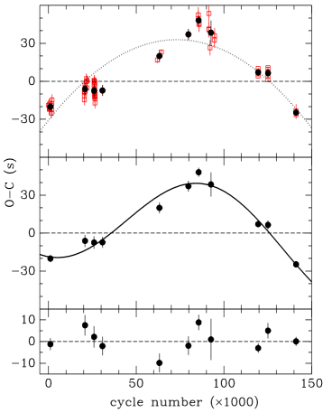
Figure 1: The O$-$C diagram of HT Cas with respect to the linear ephemeris of Table 3. The individual timings from the literature and eclipse timings measured from our light curves are shown as open squares, while the average timings of Table 2 are denoted by solid circles. The dotted line in the upper panel depicts the best-fit quadratic ephemeris while the solid line in the middle panel shows the best-fit linear plus sinusoidal ephemeris of Table 3. The lower panel displays the residuals with respect to the linear plus sinusoidal ephemeris of the middle panel.

A search for variable cycle period or for harmonics of the main cycle period (by performing separated fits to different parts of the data set) is not conclusive in this case because of the relatively short time span of the data in comparison to the cycle period. However, the eclipse timings show systematic and significant deviations from the best-fit linear plus sinusoidal ephemeris. The fact that $\chi^{2}_{\nu}>1$ emphasizes that the linear plus sinusoidal ephemeris is not a complete description of the data, perhaps signaling that the period variation is not sinusoidal or not strictly periodic.

3 Discussion

Our results reveals that the orbital period of HT Cas shows conspicuous period changes of semi-amplitude $\sim$ 40 s which seems to repeat on a time-scale of about 36 yr. The present work increases the sample of eclipsing CVs in which orbital period modulations were observed and motivated us to update the comparison of cyclical period changes of CVs above and below the period gap performed by Baptista et al. (2003).

3.1 Orbital period modulations in CVs

This section reviews the current observational picture on the detection of cyclical period changes in eclipsing CVs. We first address the observational requirements needed to allow detection of cyclical period modulations and then discuss the observational scenario which emerges when a complete sample is constructed based on these requirements. Cyclical orbital period changes are seen in many eclipsing CVs (see Baptista et al. 2003). The cycle periods range from 5 yr in IP Peg (Wolf et al 1993) to about 36 yr in HT Cas, whereas the amplitudes are in the range $10-10^{2}$ s.

A successful detection of these cyclical period changes demands an (O$-$C) diagram covering at least one cycle of the modulation (i.e., at least about a decade of observations) and that the uncertainty in the (annually averaged) eclipse timings is smaller than the amplitude of the period modulation to allow a clean detection of the latter. Therefore, decade-long time coverage and high precision eclipse timings (better than 10 s and 20 s, respectively for systems below and above the period gap) are basic requirements. A third key aspect concerns the time sampling of the observations. An (O$-$C) diagram constructed from sparse and infrequent eclipse timing measurements may easily fail to reveal a cyclical period change. Figure 2 illustrates this argument. It shows synthetic (O$-$C) diagrams constructed from a period modulation of 20 yr and amplitude 50 s (dotted line). Gaussian noise of amplitude 5 s was added to the annual timings to simulate the typical uncertainties of a real data set. The best-fit ephemeris is indicated by a solid curve/line in each case. The upper panel shows the case of poor data sampling. The gaps around eclipse cycles $\sim 30000$ and $60000-100000$ mask the period modulation and the avaliable data (solid circles) is best fit by a linear ephemeris (solid line). HT Cas itself is a good example of the poor sampling case. The revised linear ephemeris of Feline et al. (2005) was based on a sparsely sampled (O$-$C) diagram. If the timings of Wood et al. (1995), Mukai et al. (1997) and Ioannou et al. (1999) were included in their diagram the orbital period modulation would have become clear.

Figure 2: Influence of data sampling (upper panel), time coverage (middle panel) and accuracy of the eclipse timings (lower panel) in the detection of orbital period modulations. The dotted line represents (O$-$C) values constructed from a period modulation of 20 yr and amplitude 50 s (20 s in the lower panel). Gaussian noise of amplitudes 5 s (upper and middle panels) and 20 s (lower panel) were added to the (annually sampled) timings to simulate the uncertainties of a real data set. The solid line depicts the best-fit ephemeris obtained for the synthetic data used (solid circles) to illustrate each case.

The middle panel of Fig. 2 illustrates the effect of the time coverage on the detection of a period modulation. In this case the observations cover only about half of the cycle period (solid circles), leading to an incorrect inference of a long-term orbital period decrease (solid curve). A longer baseline is needed to allow identification of the cyclical nature of the period changes. Z Cha is an illustrative example of this case. Robinson et al. (1995) inferred a significant period increase from an (O$-$C) diagram covering 18 yr of observations. Only when the time coverage was increased to 30 yr the cyclical behavior of the period changes became clear (Baptista et al. 2002).

The lower panel of Fig. 2 shows how the accuracy of the eclipse timings affect the ability to detect period modulations. In this case the amplitude of the modulation was reduced to match the larger uncertainty of the eclipse timings (20 s). The period modulation is lost in the noise, despite the fact that the (O$-$C) diagram has good sampling and time coverage (solid circles), and the best-fit ephemeris is the linear one (solid line). FO Aqr, with inclination $i\sim 70^{\circ}$ and grazing eclipses (Hellier et al. 1989), may be an example of this case. The large uncertainty of its eclipse timings ($\sim 180$ s) is enough to mask cyclical period modulations of amplitude similar to those seen in other eclipsing CVs.

In summary, in order to be able to detect a period modulation one needs a well-sampled (one data point every 1$-$3 yr, no big gaps) (O$-$C) diagram covering at least a decade of observations, constructed from precise eclipse timings (uncertainty $\lower 2.15277pt\hbox{$\;\buildrel<\over{\sim}\;$}20$ s).

In order to construct a sample according to these requirements, we searched the CVcat database for all eclipsing CVs with inclination $i\geq 70^{\circ}$. The accuracy of eclipse timings below this limit is not enough to allow detection of period modulations with amplitudes $\lower 2.15277pt\hbox{$\;\buildrel<\over{\sim}\;$}200$ s. We find 14 eclipsing CVs satisfying the above criteria, 6 systems below and 8 systems above the period gap. They are listed in Table 4. All systems in the sample show cyclical period changes. With the inclusion of HT Cas, there is presently no CVs with well sampled and precise (O$-$C) diagram covering more than a decade of observations that do not show cyclical period changes. This underscores the conclusion of Baptista et al. (2003) that cyclical period changes seem a common phenomenon in CVs, being present equally among systems above and below the period gap.

Table 4: Observed orbital period modulations in CVs

Object	$P_{{\rm orb}}$	$P_{{\rm mod}}$	$\Delta P/P$	Ref.
	(hr)	(yr)	($\times 10^{-6}$)
V4140 Sgr	1.47	6.9	0.93	1
V2051 Oph	1.50	22.0	0.30	1
OY Car	1.51	35.0	0.52	2
EX Hya	1.64	17.5	0.55	3
HT Cas	1.77	36.0	0.44	This work.
Z Cha	1.79	28.0	0.85	4
IP Peg	3.80	4.7	8.00	5
U Gem	4.17	8.0	3.00	6
DQ Her	4.65	13.7	2.00	7
UX UMa	4.72	7.1, 10.7, 30.4∗	2.60	8
T Aur	4.91	23.0	3.10	9
EX Dra	5.03	5.0	7.90	10
RW Tri	5.57	7.6, 13.6∗	2.10	11
AC Cnc	7.21	16.2	5.50	12
$\ {}^{\ast}$Multiperiodic (the best determined periodicities are considered).
References: (1) Baptista et al. 2003; (2) Greenhill et al. 2006;
(3) Hellier & Sproats 1992; (4) Baptista et al. 2002; (5) Wolf et
al. 1993; (6) Warner 1988; (7) Zhang et al. 1995; (8) Rubenstein
et al. 1991; (9) Beuermann & Pakull 1984; (10) Shafter &
Holland 2003; (11) Robinson et al. 1991; (12) Qian et al. 2007b.

Apsidal motion is not a viable explanation for such period changes because the orbital eccentricity for close binaries is negligible. The presence of a third body in the system has often been invoked as an alternative explanation. However, a light-time effect implies a strictly periodic modulations in orbital period, which is usually not observed when data covering several cycles of the modulation are available. If one is to seek a common explanation for the orbital period modulation seen in CVs, then all periodic effects (such as a third body in the system) must be discarded, since the observed period changes in several of the systems (e.g., UX UMa, RW Tri, V2051 Oph) are cyclical but clearly not strictly periodic.

The best current explanation for the observed cyclical period modulation is that it is the result of a solar-type magnetic activity cycle in the secondary star. Amongst several mechanisms proposed to explain such modulations, the hypothesis of Applegate (1992) seems the most plausible. It relates the orbital period modulation to the operation of a hydromagnetic dynamo in the convective zone of the late-type component of close binaries. More precisely, Applegate’s hypothesis assumes that a small fraction of the internal angular momentum of the active component is cyclically exchanged between an inner and an outer convective shell due to a varying internal magnetic torque. This affects the oblateness and the gravitational quadrupole moment of the active component, which oscillates around its mean value. When the quadrupole moment is maximum, the companion star feels a stronger gravitational force, so that it is forced to move closer and faster around the centre of mass, thus attaining the minimum orbital period. On the other hand, when the quadrupole is minimum, the orbital period exhibits its maximum. Lanza et al. (1998) and Lanza & Rodonò (1999) have elaborated more on this idea. The model was applied to a sample of CVs by Richman et al. (1994). The fractional period change $\Delta P/P$ is related to the amplitude $\Delta(O-C)$ and to the period $P_{{\rm mod}}$ of the modulation by (Applegate 1992),

$$\frac{\Delta P}{P}=2\pi\,\frac{\Delta(O-C)}{P_{\rm mod}}=4\pi\,\frac{A}{C}\;.$$ (1)

Using the values of $A$ and $C$ in Tables 3, we find $\Delta P/P=4.4\times 10^{-7}$ for HT Cas. The values of $\Delta P/P$ for all the CVs in our sample are listed in the fourth column of Table 4.

The critical aspect of Applegate’s hypothesis is the connection of his model of gravitational quadrupole changes to a realistic cyclic dynamo model capable of produce such modulations. In this regard, Rüdiger et al. (2002) presented an $\alpha^{2}$ dynamo model for RS CVn stars, adding a dynamo mechanism to Applegate’s model. Also, theoretical improvements and observational constrains appeared recently in the literature in an attempt to overcome the limitations faced when Applegate’s model is applied to RS CVn stars (Lanza & Rodonò 2002, 2004; Lanza 2005, 2006a, 2006b). All these results can be scaled to CVs above the period gap because their secondaries also have convective envelopes.

On other hand, secondaries of CVs below the gap are thought to be fully convective (i.e, masses $M_{2}<0.3\,M_{\odot}$). Because fully convective stars have no overshoot layer, the usual dynamo mechanisms cannot be at work in these stars (Dobler 2005). However, isolated late-type main sequence stars (spectral type M5 and later) show indications of the presence of strong magnetic fields (Hawley 1993; Baliunas et al. 1995; West et al. 2004). Moreover, if magnetic activity in the secondary star is used as an explanation for the observed period modulations, the CVs below the period gap represent the first sample of fully convective dwarfs with magnetic cycles known. Alternative small-scale dynamo models have been proposed to sustain magnetic fields and induce magnetic activity cycles in fully convective stars (Durney et al. 1993; Haugen et al. 2004; Brandenburg et al. 2005; Dobler 2005 and references therein). These models indicate that an overshoot layer is not a necessary ingredient for the generation of large scale magnetic fields.

The common occurrence of $P_{{\rm orb}}$ modulations in CVs is consistent with the results of Ak et al. (2001). They found cyclical variations in the quiescent magnitude and outburst interval of a sample of CVs above and below the period gap, which they attributed to solar-type magnetic activity cycles in the secondary stars. They also found no correlation of the cycle period with the rotation regime of the secondary star (i.e., orbital period, for the phase-locked secondary stars in CVs). Considering the period modulations of a variety of close binary systems, Lanza & Rodonò (1999) found similar observational evidence for system above and below the period gap.

3.2 A comparison of the observed orbital period modulations above and below the period gap

Given the sample of well observed CVs which exhibit cyclical orbital period changes, this section attempts to quantify the common behavior as well as to address the systematic differences between the observed modulations in systems above and below the period gap. We extended the comparison by considering the period modulations observed in other longer-period close binaries (Algols, RS CVn and W UMa stars). Their magnetic activity should resemble, in some sense, the magnetic activity of the CVs above the gap since they also have a late-type (active) component with a convective envelope.

Figure 3 shows a diagram of the fractional period change $\Delta P/P$ versus the angular velocity $\Omega$ $=2\pi/P_{{\rm orb}}$ of the active, late-type component star in close binaries (rotation is a key ingredient of the dynamo action, see Lanza & Rodonò 1999). It includes data from the 14 eclipsing CVs listed in Table 4. The period gap is indicated by vertical dashed lines. The open triangles depict $\Delta P/P$ values for other close binaries with cyclical period modulations (Lanza & Rodonó 1999; Qian et al. 1999, 2000a, 2000b, 2002, 2004, 2005, 2007a; Lanza et al. 2001; Kang et al. 2002; Qian 2002a, 2002b, 2003; Yang & Liu 2002, 2003a, 2003b; Zavala et al. 2002; Çakırlı et al. 2003; Kim et al. 2003; Qian & Boonrucksar 2003; Afşar et al. 2004; Lee et al. 2004; Qian & Yang 2004; Yang et al. 2004, 2007; Zhu et al. 2004; Borkovits et al. 2005; Qian & He 2005; Erdem et al. 2007; Pilecki et al. 2007; Szalai et al. 2007). Systems with independent evidence that the observed (O$-$C) modulations can be explained by a third body were excluded (actually, it is not possible to exclude the possibility that the observed modulation of some of the systems plotted may still be caused by a third body. However, for most of the systems the observation of the modulation covers more than one cycle and there is some indication that the variation is non-periodic). There is a clear correlation between the fractional period change and the angular velocity, which can be expressed by a relationship of the type $\Delta P/P\propto\Omega^{\gamma}$ for all close binaries above the period gap. A linear least-squares fit yields $\gamma=-0.7\pm 0.1$. The best-fit solution and the 3-$\sigma$ confidence level are indicated by a solid and dotted lines, respectively, in Fig. 3.

Figure 3: Diagram of the fractional period change $\Delta P/P$ versus the angular velocity $\Omega$ of the active component star in short-period CVs (filled circles), long-period CVs (filled squares) and other close binaries from the literature (open triangles). The period gap is represented by the vertical dashed lines. The best-fit linear relation and its 3-$\sigma$ confidence level are shown as solid and dotted lines, respectively. The diagram includes the measurements of the CVs listed in Table 4.

We find that the average fractional period changes of the short-period CVs ($\overline{\Delta P/P}\simeq 8\times 10^{-7}$) are systematically smaller than those of the long-period CVs ($\overline{\Delta P/P}\simeq 4\times 10^{-6}$) by a factor $\simeq 5$. The mean value of $\Delta P/P$ of the short-period CVs is more than 3-$\sigma$ below the value expected from the linear relation inferred for the other, longer period close binaries. An attempt to simultaneously explain CVs above and below the gap by vertically displacing the $\Delta P/P$ versus $\Omega$ fitted relation results in a poor fit with high $\chi^{2}_{\nu}$. Similarly, including the CVs below the period gap in the sample degrades the fit and significantly increases the $\chi^{2}_{\nu}$. Despite the small sample (14 objects), there is a statistically significant difference between the $\Delta P/P$ values of the CVs above and below the period gap. This difference cannot be eliminated even if we take into account the fitted $\Delta P/P$ versus $\Omega$ relation that predicts decreasing $\Delta P/P$ values for increasing $\Omega$. Thus, we are forced to conclude that the CVs below the period gap do not fit the relation valid for the binaries above the period gap.

If the interpretation of cyclical period changes as the consequence of a solar-like magnetic activity cycle is correct, the existence of cyclical period changes in binaries with fully convective active stars is an indication that these stars do have magnetic fields, not only capable of inducing strong chromospheric activity (e.g, Hawley 1993), but also measurable magnetic activity cycles (Ak et al. 2001; this paper). On the other hand, the fact that the fractional period changes of binaries with fully convective stars is systematically smaller than those of stars with radiative cores is a likely indication that a different mechanism is responsible to generate and sustain their magnetic fields. In this regard, the observed lower $\Delta P/P$ values yield a useful constrain to any model that might be developed to account for magnetic fields in fully convective stars.

The investigation of cyclical period changes in CVs will greatly benefit from the increase in the (presently small) sample of systems with well-sampled (O$-$C) diagrams covering more than a decade of observations. This demands the patient but systematic collection of precise eclipse timings over several years. It is worth mentioning that there is a good number of well-known eclipsing CVs for which a few years of additional eclipse timings observations would suffice to overcome the ambiguities illustrated in Fig. 2 and to allow statistically significant detection of period modulations. We also remark that none of the systems inside the period gap has been yet observed for long enough time to allow identification of cyclical period changes. It would be interesting to check whether these systems will fit the $\Delta P/P\propto\Omega^{-0.7}$ relation or will display a behavior similar to that of the CVs below the period gap.

In order to explain the CV period gap, the disrupted braking model predicts a significant reduction in magnetic braking efficiency between the systems above and below the period gap (Hameury et al. 1991). The observed difference in $\Delta P/P$ between CVs above and below the period gap could be used to test this prediction if a connection between fractional period changes and braking efficiency could be established.

- (1) Afşar, M., Heckert, P. A., İbanoǧlu, C. 2004, A&A, 420, 595
- (2) Ak, T., Ozkan, M. T., & Mattei, J. A. 2001, A&A, 369, 882
- (3) Andronov, N., & Pinsonneault, M. H. 2004, ApJ, 614, 326
- (4) Andronov, N., Pinsonneault, M., & Sills, A. 2003, ApJ, 582, 358
- (5) Applegate, J. H. 1992, ApJ, 385, 621
- (6) Applegate, J. H., & Patterson J. 1987, ApJ, 322, L99
- (7) Baliunas, S. L., Donahue, R. A., Soon, W. H., et al. 1995, ApJ, 438, 269
- (8) Baptista, R., Borges, B. W., Bond, H. E., et al. 2003, MNRAS, 345, 889
- (9) Baptista, R., Jablonski, F. J., Oliveira, E., et al. 2002, MNRAS, 335, L75
- (10) Beuermann, K., & Pakull, M. W. 1984, A&A, 136, 250
- (11) Borkovits, T., Elkhateeb, M. M., Csizmadia, S., et al. 2005, A&A, 441, 1087
- (12) Brandenburg, A., Haugen, N. E. L., Käpylä, P. J., & Sandin, C. 2005, Astron. Nachr., 326, 174
- (13) Çakırlı, Ö., İbanoǧlu, C., Djurašević, G. et al. 2003, A&A, 405, 733
- (14) Dobler, W. 2005, Astron. Nachr., 326, 254
- (15) Durney, B. R., De Young, D. S., & Roxburgh, I. W. 1993, Sol. Phys., 145, 207
- (16) Erdem, A., Doğru, S. S., Bakış, V., & Demircan, O. 2007, Astron. Nachr., 328, 543
- (17) Feline, W. J., Dhillon, V. S., Marsh, T. R., Watson, C. A., & Littlefair, S. P. 2005, MNRAS, 364, 1158
- (18) Greenhill, J. G., Hill, K. M., Dieters, S. et al. 2006, MNRAS, 372, 1129
- (19) Hameury, J. M., King, A. R., & Lasota, J. P. 1991, A&A, 248, 525
- (20) Haugen, N. E., Brandenburg, A., & Dobler, W. 2004, Phys. Rev. E, 70, 016308
- (21) Hawley, S. L. 1993, PASP, 105, 955
- (22) Hellier, C., & Sproats, L. N. 1992, IBVS, 3724, 1
- (23) Hellier, C., Mason, K. O., & Cropper, M. 1989, MNRAS, 237, 39P
- (24) Horne, K., Wood, J. H., & Stiening, R. F. 1991, ApJ, 378, 271
- (25) Ioannou, Z., Naylor, T., Welsh, W. F., et al. 1999, MNRAS, 310, 398
- (26) Kang, Y. W., Oh, K.-D., Kim, C.-H., et al. 2002, MNRAS, 331, 707
- (27) Kim, C.-H., Lee, J. W., Kim, H.-I., Kyung, J.-M., & Koch, R. H. 2003, AJ, 126, 1555
- (28) Knigge, C. 2006, MNRAS, 373, 484
- (29) Lanza, A. F. 2005, MNRAS, 364, 238
- (30) Lanza, A. F. 2006a, MNRAS, 369, 1773
- (31) Lanza, A. F. 2006b, MNRAS, 373, 819
- (32) Lanza, A. F., & Rodonò, M. 1999, A&A, 349, 887
- (33) Lanza, A. F., & Rodonò, M. 2002, Astron. Nachr., 323, 424
- (34) Lanza, A. F., & Rodonò, M. 2004, Astron. Nachr., 325, 393
- (35) Lanza, A. F., Rodono, M., & Rosner, R. 1998, MNRAS, 296, 893
- (36) Lanza, A. F., Rodonò, M., Mazzola, L., & Messina, S. 2001, A&A, 376, 1011
- (37) Lee, J. W., Kim, C.-H., Han, W., Kim, H.-I., & Koch, R. H. 2004, MNRAS, 352, 1041
- (38) Matese, J. J., & Whitmire, D. P. 1983, A&A, 117, L7
- (39) Patterson, J. 1984, ApJS, 54, 443
- (40) Patterson, J., Kemp, J, Richman, H. R., et al. 1998, PASP, 110, 415
- (41) Pilecki, B., Fabrycky, D., & Poleski, R. 2007, MNRAS, 378, 757
- (42) Pringle, J. 1975, MNRAS, 170, 633
- (43) Qian, S.-B. 2002a, A&A, 387, 903
- (44) Qian, S.-B. 2002b, MNRAS, 336, 1247
- (45) Qian, S.-B. 2003, A&A, 400, 649
- (46) Qian, S.-B., & Boonrucksar, S. 2003, PASJ, 55, 499
- (47) Qian, S.-B., & He, J.-J. 2005, PASJ, 57, 977
- (48) Qian, S.-B., & Yang, Y.-G. 2004, AJ, 128, 2430
- (49) Qian, S.-B., Liu, Q.-Y., & Yang, Y.-L. 1999, Ap&SS, 266, 529
- (50) Qian, S.-B., Liu, Q.-Y., Yang, Y.-L., & Yuan, L.-L. 2000a, Chinese Astron. Astrophys., 24, 331
- (51) Qian, S.-B., Liu, Q.-Y., & Tan, W. 2000b, Ap&SS, 274, 859
- (52) Qian, S.-B., Liu, D., Tan, W., & Soonthornthum, B. 2002, AJ, 124, 1060
- (53) Qian, S.-B., Soonthornthum, B., Xiang, F.-Y., Zhu, L.-Y., & He, J.-J. 2004, Astron. Nachr., 325, 714
- (54) Qian, S.-B., He, J.-J., Xiang, F.-Y., Ding, X., & Boonrucksar, S. 2005, AJ, 129, 1686
- (55) Qian, S.-B., Xiang, F.-Y., Zhu, L.-Y., et al. 2007a, AJ, 133, 357
- (56) Qian, S.-B., Dai, Z.-B., He, J.-J., et al. 2007b, A&A, 466, 589
- (57) Rappaport, S., Verbunt, F., & Joss, P. C. 1983, ApJ, 275, 713
- (58) Richman, H. R., Applegate, J. H., & Patterson, J. 1994, PASP, 106, 1075
- (59) Robertson, J. W., & Honeycutt, R. K. 1996, AJ, 112, 2248
- (60) Robinson, E. L., Shetrone, M. D., & Africano, J. L. 1991, AJ, 102
- (61) Robinson, E. L., Wood, J. H., Bless, R. C., et al. 1995, ApJ, 443, 295
- (62) Rubenstein, E. P., Patterson, J., & Africano, J. L. 1991, PASP, 103, 1258
- (63) Rüdiger, G., Elstner, D., Lanza, A. F., & Granzer, T. 2002, A&A, 392, 605
- (64) Stumpff, P. 1980, A&A, 41, 1
- (65) Szalai, T., Kiss, L. L., Mészáros, S., Vinkó, J., & Csizmadia, S. 2007, A&A, 465, 943
- (66) Warner, B. 1995, Cataclysmic Variable Stars (Cambridge University Press, Cambridge)
- (67) Warner, B. 1988, Nature, 336, 129
- (68) West, A. A., Hawley, S. L., Walkowicz, L. M., et al. 2004, AJ, 128, 426
- (69) Wolf, S., Mantel, K. H., Horne, K., et al. 1993, A&A, 273, 160
- (70) Wood, J. H., Irwin, M. J., & Pringle, J. E. 1985, MNRAS, 214, 475
- (71) Wood, J. H., Naylor, T., Hassall, B. J. M., & Ramseyer, T. F. 1995, MNRAS, 273, 772
- (72) Yang, Y.-L., & Liu, Q.-Y. 2002, AJ, 124, 3358
- (73) Yang, Y.-L., & Liu, Q.-Y. 2003a, AJ, 126, 1960
- (74) Yang, Y.-L., & Liu, Q.-Y. 2003b, PASP, 115, 748
- (75) Yang, Y.-G., Qian, S.-B., & Zhu, C.-H. 2004, PASP, 116, 826
- (76) Yang, Y.-G., Dai, J.-M., Yin, X.-G., & Xiang, F.-Y. 2007, AJ, 134, 179
- (77) Zavala, R. T., McNamara, B. J., Harrison, T. E., et al. 2002, AJ, 123, 450
- (78) Zhang, E.-H., Robinson, E. L., & Nather, R. E. 1986, ApJ, 305, 740
- (79) Zhang, E., Robinson, E. L., Stiening, R. F., & Horne, K. 1995, ApJ, 454, 447
- (80) Zhu, L.-Y., Qian, S.-B., & Xiang, F.-Y. 2004, PASJ, 56, 809