Voltage profile and four terminal resistance of an interacting quantum wire.

Abstract

We investigate the behavior of the four-terminal resistance $R_{4pt}$ in a quantum wire described by a Luttinger liquid in two relevant situations: (i) in the presence of a single impurity within the wire and (ii) under the effect of asymmetries introduced by disordered voltage probes. In the first case, interactions leave a signature in a power law behavior of $R_{4pt}$ as a function of the voltage $V$ and the temperature $T$. In the second case interactions tend to mask the effect of the asymmetries. In both scenarios the occurrence of negative values of $R_{4pt}$ is explained in simple terms.

The proposal of a fundamental relation between the two terminal conductance $G$ and the universal quantum $G_{0}=e^{2}/h$ is one of the milestones of electronic quantum transport in mesoscopic systems conwinonin1 ; conwinonin2 . For non-interacting electrons, such a relation explicitly reads $G=nG_{0}$, being $n$ the number of electronic channels conwinonin2 . The same relation has been later theoretically and experimentally probed to be also valid in the case of wires of interacting electrons of finite length ideally attached to non-interacting leads conwiint ; conwiex .

Experiments in single-wall nanotubes (SWNTs), ropes of SWNTs and also in multiple-wall nanotubes (MWNTs) condnanot12 have, instead, identified that the tunneling conductance to metallic contacts, $G_{t}$ follows a power law behavior with the voltage $V$ $G_{t}\propto V^{\alpha}$ at low temperature $T$, and $G_{t}\propto T^{\alpha}$ for low $V$. The exponent ${\alpha}$ being a function of the forward electron-electron (e-e) interaction $g$. These features can be understood within the framework of a Luttinger liquid (LL) theory by means of theoretical treatments conlut going beyond linear response in $V$ and $T$.

Recently, a combined structure of MWNTs and SWNTs has been used to analyze the behavior of the four-point resistance $R_{4pt}$ of a SWNT nano4pt . The total resistance of a mesoscopic system in a two terminal setup contains the component $1/G_{0}$ due to the coupling to the reservoirs. Instead, $R_{4pt}$ is expected to characterize the genuine resistance of the sample. For non-interacting electrons at low $V$ and zero temperature, Büttiker has elaborated the concept of the multi-terminal resistance within scattering-matrix theory (SMT) but4pt , emphasizing the role of the symmetries. Although a naive expectation would be $R_{4pt}\geq 0$, this theory predicts also the possibility of $R_{4pt}<0$ as a consequence of quantum interference effects. This remarkable feature has been experimentally observed nano4pt ; pict .

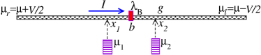
Figure 1: Sketch of the setup: A voltage $V$ is imposed on a Luttinger liquid with a backscattering impurity of strength $\lambda_{B}$, through the chemical potentials for the left and right movers: $\mu_{r,l}=\mu\pm V/2$. Two voltage probes are connected at the positions $x_{1},x_{2}$. The corresponding chemical potentials $\mu_{1,2}$ are fixed by the condition of zero current through the contacts.

While the consequences of elastic scattering due to impurities can be analyzed in terms of non-interacting electrons, the role of the e-e interaction in the behavior of $R_{4pt}$ remains an open question. The proper evaluation of this quantity implies dealing with a multi-terminal setup as the one of Fig. 1, which is difficult to implement within theoretical approaches like those of Refs. conlut, ; egger, ; dolc, . Previous multi-terminal treatments in LL rely in the effective reduction to a non-interacting model by recourse to a Hartree-Fock decoupling of the interaction term lao or focus in linear response in $V$ chamon . In this work we use Keldysh non-equilibrium Green’s functions, which is a convenient framework to tackle multi-terminal geometries by exactly treating the e-e interaction while going beyond linear response. We analyze two relevant ingredients giving rise to a non-trivial behavior of the local potential $\mu_{j}$ and $R_{4pt}$: (i) the presence of an impurity in the wire and (ii) a clean wire probed by disordered leads with asymmetric densities of states.

We consider the setup sketched in Fig. 1, which consists in a quantum wire described by a Tomonaga-Luttinger model under the influence of a voltage $V$. Two reservoirs are in contact with the wire at the points $x_{1},x_{2}$ through very weak (“non invasive”) tunneling constants, their chemical potentials $\mu_{1},\mu_{2}$ satisfy the condition of a vanishing current through the ensuing contacts. In this way, a continuous current $I$ flows through the wire, and

$$\frac{R_{4pt}}{R_{2pt}}=\frac{\mu_{1}-\mu_{2}}{V}.$$ (1)

In the case of an ideal and clean wire with identical non invasive probes, a simple analysis of the symmetries of the setup leads to $R_{4pt}=0$. The full system is described by the action $S=S_{wire}+S_{imp}+S_{res}+S_{cont}$, where $S_{res}$ describes the two reservoirs that constitute the voltage probes and $S_{wire}$ is expressed in terms of right ($r$) and left ($l$) movers (in our system of units $\hbar=v_{F}=e=1$):

$$S_{wire} =\int dx\,dt\,\{\psi_{r}^{\dagger}[i(\partial_{t}+\partial_{x})-\mu_{r}]\psi_{r}+$$ (2)

$$+\psi_{l}^{\dagger}[i(\partial_{t}-\partial_{x})-\mu_{l}]\psi_{l}-g[\psi_{r}^{\dagger}\psi_{r}+\psi_{l}^{\dagger}\psi_{l}]^{2}\},$$

where $g$ is the Luttinger e-e interaction in the forward channel while $\mu_{r}=\mu+V/2$ and $\mu_{l}=\mu-V/2$. The effect of the impurity is contained in the back-scattering interaction:

$$S_{imp} = \lambda_{B}\int dx\,dt\,\delta(x-b)\,[e^{-2ik_{F}x}\psi_{r}^{\dagger}\psi_{l}+H.c].$$ (3)

The term $S_{cont}$ represents the tunneling between the reservoirs and the wire:

$$S_{cont} = \sum_{j=1,2,\alpha,\beta=l,r}\,\,\int dx\,dt\,w_{j}\delta(x-x_{j})\times$$ (4)

$$[e^{\mp i(k_{F}+k^{\prime}_{F})x}\psi_{\alpha}^{\dagger}\chi_{\beta,j}+H.c],$$

where the fields $\chi_{\alpha,j}^{\dagger}$, with $\alpha,\beta=l,r$, $j=1,2$ denote degrees of freedom of the reservoirs. The upper and lower sign corresponds to $\alpha=r,l$, respectively. For simplicity, the dependence of the fields on $x$ and $t$ has been omitted in the above equations. At this point we carry out the gauge transformation $\psi_{l,r}^{\dagger}(x)\rightarrow e^{i\pm k_{F}x}\psi_{\alpha}^{\dagger}(x)$ where $k_{F}$ is the Fermi vector of the electrons in the wire (a similar transformation involving $k^{\prime}_{F}$ is implemented with the fields $\chi_{\alpha,j}^{\dagger}$).

The tunneling currents through the contacts to the probes read

$$I_{j}=iw_{j}\sum_{\alpha,\beta=l,r}\langle\chi_{j,\alpha}^{\dagger}(x_{j},t)\psi_{\beta}(x_{j},t)-H.c\rangle.$$ (5)

In what follows, we evaluate the currents $I_{j}$ up to the first order of perturbation theory in the tunneling amplitudes. This procedure is appropriate in the limit of weak $w_{j}$, which is a reasonable assumption for measurements of $R_{4pt}$ with ‘non-invasive’ probe leads nano4pt . Within this lowest order of perturbation theory:

$$I_{j} = 2|w_{j}|^{2}\sum_{\alpha,\beta=l,r}\int_{-\infty}^{+\infty}\frac{d\omega}{2\pi}[G_{\alpha,\beta}^{>}(x_{j},x_{j};\omega)G_{j}^{<}(\omega)$$ (6)

$$-G_{\alpha,\beta}^{<}(x_{j},x_{j};\omega)G_{j}^{>}(\omega)],$$

where $G_{\alpha,\beta}^{<,>}(\omega)$ are the Fourier transforms with respect to $t-t^{\prime}$ of the lesser and bigger Green’s functions $G_{\alpha,\beta}^{<}(x,x^{\prime};t-t^{\prime})=i\langle\psi_{\beta}^{\dagger}(x^{\prime},t^{\prime})\psi_{\alpha}(x,t)\rangle$, $G_{\alpha,\beta}^{>}(x,x^{\prime};t-t^{\prime})=-i\langle\psi_{\alpha}(x,t)\psi_{\beta}^{\dagger}(x^{\prime},t^{\prime})\rangle$, corresponding to the wire uncoupled from the probes, while $G_{j}^{>,<}(\omega)=\lambda^{>,<}_{j}(\omega)\rho_{j}(\omega)$ are the Green’s functions of the uncoupled probe reservoirs, with $\lambda^{<}_{j}(\omega)=if(\omega-\mu_{j})$, $\lambda^{>}_{j}(\omega)=-i[1-f(\omega-\mu_{j})]$, and $\rho_{j}(\omega)$ the ensuing density of states, which we assume to be identical for the two kinds of movers within these systems. The chemical potentials of the probes, $\mu_{j}$ must be fixed to satisfy $I_{j}=0$. Notice that, within this order of perturbation theory, the effect of the two probes is completely uncorrelated from one another, since interference terms between the probes and resistive effects involve second order processes in $w_{j}$ sec .

We now turn to analyze the first ingredient of interest, namely, the effect of an impurity in the wire. In terms of our model, this corresponds to consider a finite $\lambda_{B}$. We also consider a simple model for the probes, with a constant density of states $\rho_{j}(\omega)=\rho_{0}$. While the Green’s functions of the uncoupled homogeneous interacting wire are known medvoit , the evaluation of the corresponding functions in the presence of a backscattering center is a non-trivial task. Below, we indicate the lines we have followed in order to evaluate them up to the first order of perturbation theory in $\lambda_{B}$. The expressions for the lesser and bigger Green’s functions cast:

$$G^{>,<}_{\alpha\beta}(x,x^{\prime},\omega) = \delta_{\alpha\beta}\lambda^{>,<}_{\alpha}(\omega)\rho_{0,\alpha}(x-x^{\prime},\omega)+$$ (7)

$$\delta_{\overline{\alpha}\beta}\lambda_{B}\{\lambda^{>,<}_{\alpha}(\omega)\rho_{0,\alpha}(x-b,\omega)$$

$$\times[G^{R}_{0,\beta}(x^{\prime}-b,\omega)]^{*}+\lambda^{>,<}_{\beta}(\omega)$$

$$\times G^{R}_{0,\alpha}(x-b,\omega)\rho_{0,\beta}(b-x^{\prime},\omega)\},$$

with $\overline{l}=r,\overline{r}=l$, $\lambda^{<}_{\alpha}(\omega)=if(\omega-\mu_{\alpha})$, $\lambda^{>}_{\alpha}(\omega)=-i[1-f(\omega-\mu_{\alpha})]$. The spectral density

$$\rho_{0,\alpha}(x,\omega+\mu_{\alpha}) = C_{\psi}\exp{[\mp i(\frac{\omega}{v}-k_{F})x]}$$ (8)

$$\times|\omega|^{2\gamma}\phi(\gamma,2\gamma+1,\pm 2ix\frac{\omega}{v}),$$

corresponds to the clean LL uncoupled from the probes, where $v=\sqrt{1+2g/\pi}$ is the renormalized Fermi velocity and $\phi(a,b;c)$ is Kummer’s hypergeometric function. The exponent $\gamma=(K+K^{-1}-2)/4$, ($K=1/v$) is determined by $g$. The retarded Green’s functions are defined from the Kramers-Kronig relation, being $\rho_{0,\alpha}(x,\omega)=-2\mbox{Im}[G^{R}_{0,\alpha}(x,\omega)]$. In order to perform numerical computations we introduce an energy cutoff $\Lambda$ by replacing $\rho_{0,\alpha}(x,\omega+\mu_{\alpha})\rightarrow\Theta(|\omega|-\Lambda)\rho_{0,\alpha}(x,\omega+\mu_{\alpha})$. Therefore the constant $C_{\psi}$ is a function of $\Lambda$ which is determined by the sum rule $\int_{-\infty}^{+\infty}d\omega\rho_{\alpha,0}(0,\omega)=2\pi$.

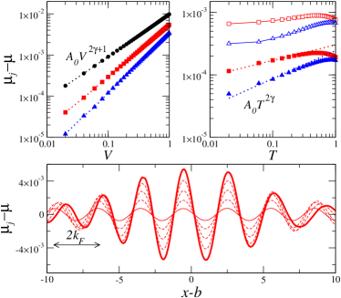
Figure 2: Behavior of the local potential $\mu_{j}$ for a wire with $\lambda_{B}=0.1$ as a function of the bias $V$ for $T=0$ and $x_{j}=-0.2$ (upper left panel) and as a function of $T$ for $V=0.2$ and $x_{j}=-0.2$ (right panel). Circles, squares and triangles correspond to $K=1,0.5,0.4$, respectively. Solid and open symbols correspond to $V=0.05,0.2$, respectively (right panel). The fits with power laws are shown in dotted lines. Lower panel: $\mu_{j}$ as a function of $x-b$ for $V=0.2,\ldots,1$ and $K=0.5$.

Substituting the above expressions in (6) gives the following result for the currents through the contacts:

$$I_{j}(x_{j}) = 2|w_{j}|^{2}\sum_{\alpha=l,r}\int_{-\infty}^{\infty}\frac{d\omega}{2\pi}[f(\omega-\mu_{j})-f(\omega-\mu_{\alpha})]$$ (9)

$$\times\rho_{j}(\omega)\rho^{eff}_{\alpha}(x_{j},\omega),$$

being

$${\rho}^{eff}_{\alpha}(x_{j},\omega) = \rho_{0,\alpha}(0,\omega)+2\lambda_{B}\mbox{Re}\{\rho_{0,\alpha}(x_{j}-b,\omega)$$ (10)

$$\times[G^{R}_{0,\overline{\alpha}}(x_{j}-b,\omega)]^{*}\},$$

the effective density of states of the $\alpha$ movers (or the $\alpha$-injectivity bufri2 ) at the position $x_{j}$ of the wire, which contains the contribution of the local density of states of the homogeneous wire, $\rho_{0,\alpha}(0,\omega)$ plus a correction due to the backscattering by the impurity. It is important to note that $I_{j}(x_{j})\propto\lambda_{B}$, while the current through the wire is $I\propto\lambda^{2}_{B}$ (see also Refs. egger ; dolc ). For $T=0$ and low $V$, the condition $I_{j}=0$ leads to

$$\mu_{j}=\mu+\frac{V}{2}\frac{\rho^{eff}_{l}(x_{j},\mu)-\rho^{eff}_{r}(x_{j},\mu)}{\rho^{eff}_{l}(x_{j},\mu)+\rho^{eff}_{r}(x_{j},\mu)},$$ (11)

where we have made use of the fact that $\rho_{j}(\omega)$ is constant and that $\rho^{eff}_{\alpha}(x_{j},\omega)\sim\rho^{eff}_{\alpha}(x_{j},\mu)$ within a small window $|\omega-\mu|\leq V/2$. Eq. (11) reduces to Eq.(37) of Ref. bufri2, for non-interacting electrons. It explicitly shows that the local potential monitors the difference between the left and right injectivities at the point $x_{j}$, relative to the total density of states at the given point. It is natural to expect that such an observable should provide valuable information on the Friedel oscillations introduced by the impurity egger ; dolc ; bufri1 ; bufri2 , as well as on the strength of the e-e interactions. In fact, a low-energy expansion of the spectral densities casts:

$$\mu_{j} \sim \mu+C_{1}\,\lambda_{B}\,\sin(2k_{F}x)\,V^{2\gamma+1},\;\;\;T=0$$

$$\mu_{j} \sim \mu+C_{2}\,\lambda_{B}\,V\sin(2k_{F}x)\,T^{2\gamma},\;\;\;V\ll T,$$ (12)

with $C_{1},C_{2}$ functions of $\gamma$.

The results of the full numerical calculation of $\mu_{j}$ from the condition of $I_{j}(x_{j})=0$ for arbitrary voltage differences and temperature, with the exact effective density $\rho^{eff}_{\alpha}(x_{j},\omega)$ (also evaluated numerically from eq.(10)), are shown in Fig. 2. At $T=0$, $\mu_{j}$ as a function of the distance to the impurity, shown in the lower panel, oscillates with the period $2k_{F}$ of the Friedel oscillations, with a voltage-dependent amplitude that follows the power law (Voltage profile and four terminal resistance of an interacting quantum wire.) (see upper left panel). For large distances to the impurity and high $V$, beyond the scope of the approximations leading to eqs. (Voltage profile and four terminal resistance of an interacting quantum wire.), the pattern shows additional structure, and the amplitude of the oscillations decreases with the distance to the impurity. The evolution of $\mu_{j}$ as the temperature increases, corresponding to two values of the voltage, is illustrated in the upper right panel of Fig. 2, where the dependence (Voltage profile and four terminal resistance of an interacting quantum wire.) is also verified within the low $T$ and low $V$ regime, with $V\ll T$. From these features we can infer the behavior of $R_{4pt}/R_{2pt}$ along the sample by simply substituting (11) in (1). In particular, we conclude that, as a function of $x$, $R_{4pt}/R_{2pt}$ should follow the pattern of Friedel oscillations, being positive or negative, depending on the points at which the probes are connected. As a function of $V$ it should be a power law with exponent $2\gamma$. As a function of $T$, it should present rapid changes within the range $T<V$ and a crossover to a power law with exponent $2\gamma$ at higher temperatures.

We now consider the second situation of interest: the wire without impurities ($\lambda_{B}=0$) but disordered probe leads. Thus, the expressions for the Green’s function of the wire reduce to the ones for the homogeneous LL while the expression for the tunneling current of eq. (6) reduces to eq. (9) with $\rho_{\alpha}^{eff}(x_{j},\omega)\equiv\rho_{\alpha,0}(0,\omega)$. While perfect metallic systems are expected to have approximately flat densities of states, impurities introduce effective barriers, generating peaks in the densities of states $\rho_{j}(\omega)$.

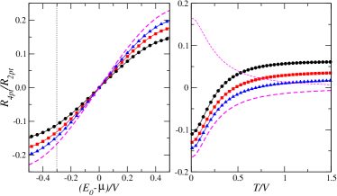
Figure 3: Four point resistance $R_{4pt}/R_{2pt}$ of a LL with interaction parameter $K$ for a bias $\mu_{r}-\mu_{l}=V$. The probe $j=1$ has a Lorentzian density of states (a resonance) with width $\Delta=0.4V$ centered at $E_{0}$. The probe $j=2$ has a constant density of states (which implies $\mu_{2}=\mu=(\mu_{l}+\mu_{r})/2$). The left panel corresponds to temperature $T=0$ and shows the changes in $R_{4pt}$ as the center of the resonance is moved around $\mu$. Circles, squares and triangles correspond to $K=0.4,0.5,0.6$, while dashed lines, to the non-interacting case ($K=1$). The right panel shows the evolution with the temperature for the value of $(E_{0}-\mu)/V=-0.3$ indicated with dotted lines in the left panel. The thin dashed line corresponds to $K=1$ and $(E_{0}-\mu)/V=0.3$.

Let us first analyze $T=0$ and probes with asymmetric density of states, such that $\rho_{j}(\omega)\sim\rho^{-}_{j}(\mu),\mu-V/2\leq\omega\leq\mu$ and $\rho_{j}(\omega)\sim\rho^{+}_{j}(\mu),\mu\leq\omega\leq\mu+V/2$. Then, the condition of a vanishing current (6) leads to:

$$\mu_{j}=\mu+\frac{V}{2}[\frac{\rho^{+}_{j}(\mu)^{\nu}-\rho^{-}_{j}(\mu)^{\nu}}{\rho^{-}_{j}(\mu)^{\nu}+\rho^{+}_{j}(\mu)^{\nu}}],$$ (13)

being $\nu=1/(2\gamma+1)$. For probes with symmetric densities of states, we get $\mu_{j}=\mu$ and $R_{4pt}=0$. Instead, for an asymmetric density of states, the potential drop between the highest potential $r$ and the probe $j$ is lower (higher) than the one between $j$ and $l$ for $\rho^{-}_{j}(\mu)>\rho^{+}_{j}(\mu)$ ($\rho^{-}_{j}(\mu)<\rho^{+}_{j}(\mu)$), respectively, which reflects the fact that the larger the spectral weight of the probe, the larger the ability of that element to introduce resistive effects. For finite temperature and very low voltage such that $T\gg V$, it can be verified that $\mu_{j}=\mu,j=1,2$ and $R_{4pt}=0$.

Therefore, asymmetric densities of states of at least one of the probes together with the condition $\rho_{1}(\omega)\neq\rho_{2}(\omega)$ would lead to a non vanishing $R_{4pt}$ when $T<V$. An example is analyzed in Fig. 3. We consider a Breit-Wigner model for one of the probes, assuming a single resonance within the window of width $V$ centered around $\mu$: $\rho_{1}(\omega)=A_{1}/[(\omega-E_{0})^{2}+\Delta]$, and a constant density of states $\rho_{2}=A_{2}$ for the other probe, where $A_{1},A_{2}$ are normalization constants and $\mu-V/2\leq E_{0}\leq\mu+V/2$. Under these conditions $\mu_{2}=\mu$, while $\mu_{1}$ is determined to satisfy $I_{1}=0$. Results for the corresponding relative resistance $R_{4pt}/R_{2pt}=(\mu_{1}-\mu_{2})/V$ are shown in Fig. 3. The left panel corresponds to temperature $T=0$. When the center of the resonance $E_{0}$ coincides with the mean chemical potential $\mu$, the spectral weight spreads out symmetrically around this point. Thus, $\rho_{1}^{+}(\mu)=\rho_{1}^{-}(\mu)$ and $\mu_{1}=\mu$, then $R_{4pt}=0$. As the center of the resonance moves to lower energies, so does $\mu_{1}$ and $R_{4pt}$ becomes negative. Conversely, for $E_{0}>\mu$, it is obtained $R_{4pt}>0$. Remarkably, interactions tend to mask the structure observed in the non-interacting case (with $K=1$). The behavior of $R_{4pt}$ as a function of the temperature is shown in the right panel for the case $(E_{0}-\mu)/V=-0.3$. Notice that the cases with $(E_{0}-\mu)/V>0$ can be obtained from the ones with $(E_{0}-\mu)/V<0$ by simply transforming $R_{4pt}\rightarrow-R_{4pt}$ in the figure. In all the cases, there is a range of temperature $T<V$, where $R_{4pt}$ experiments significant changes.

To conclude, let us comment on the theoretical and experimental impact of our results. When an impurity is in the wire, it induces Friedel oscillations that manifest themselves in the local voltage and $R_{4pt}$. The interactions leave a clear signature in the power law behavior $R_{4pt}/R_{2pt}\propto V^{2\gamma}$ and $R_{4pt}/R_{2pt}\propto T^{2\gamma}$. Interestingly, the exponent is different from the one predicted in Ref. dolc, for the two terminal conductance of a LL with an impurity. This result has a significant conceptual weight since it constitutes a concrete example of the fact that different fundamental processes contribute to each of these quantities ($R_{4pt}/R_{2pt}\propto\lambda_{B}$ while $G\propto\lambda_{B}^{2}$). Therefore, a genuine multiterminal setup is essential to evaluate $R_{4pt}$. For impurities in the probes and an asymmetric configuration, $R_{4pt}$ is determined by the way in which the density of states of the probe is distributed within an energy window of width $V$ centered in $\mu$, while the e-e interactions play a milder role. In both cases, the behavior of $R_{4pt}$ as a function of temperature at a sizable $V$, is highly non universal and exhibits significant changes in the range $T<V$. These results should help to provide a theoretical framework to further analyze experimental data in SWNT, like those of Ref. nano4pt, as well as to guide additional experiments along that line in the future.

We thank A.Bachtold, M.Büttiker and C.Chamon for useful discussions. We acknowledge support from CONICET, Argentina, FIS2006-08533-C03-02 and PIP-6157; PIA-11X386 UNLP, Argentina; the “RyC” program from MCEyC, grant DGA for Groups of Excellence and AUIP of Spain.

References

- (1) R. Landauer, Philos. Mag. 21 863 (1970).
- (2) M. Büttiker, et al , Phys. Rev. B 31, 6207 (1985).
- (3) W. Apel and T. M. Rice, Phys. Rev. B 26 7063 (1982); C. Kane and M. P. A. Fisher, Phys. Rev. B 46 15233 (1992);D. Maslov and M. Stone, Phys. Rev. B 52 R5539 (1995); V. V. Ponomarenko, Phys. Rev. B 52 R8666 (1995); I Safi and H. J. Schulz, Phys. Rev. B 52 R17040 (1995).
- (4) S. Tarucha, T. Honda and T. Saku, Solid State Comm. 94 413 (1995); N. Agrait,et al, Physics Reports 81 377 (2003) and references therein.
- (5) M. Bockrath, et al , Nature 397, 598 (1999). M. Monteverde and M. Nuñez Regueiro, Phys. Rev. Lett. 94, 235501 (2005).
- (6) R. Egger and A. Gogolin, Phys. Rev. Lett. 79, 5082 (1997).
- (7) M. Büttiker, Phys. Rev. Lett. 57 1761 (1986); M. Büttiker, IBM J. Res, 32, 317 (1988).
- (8) B. Gao, et al , Phys. Rev. Lett. 95 196802 (2005).
- (9) R. de Picciotto, et al , Nature 411, 51 (2001).
- (10) R. Egger and H. Grabert, Phys. Rev. Lett. 77, 538 (1996); Phys. Rev. B 58, 10761 (1998).
- (11) F. Dolcini et al, Phys. Rev. B 71, 165309 (2005).
- (12) S. Lal, S. Rao, and D. Sen, Phys. Rev. B 66, 165327 (2002); S. Das, S. Rao, and D. Sen, Phys. Rev. B 70, 085318 (2004).
- (13) C. Chamon,et al, Phys. Rev. Lett. 91 206403 (2003); C-Y Hou and C. Chamon, cond-mat/0801.3824, references therein.
- (14) V. A. Gopar,et al, Phys. Rev. B 50, 2502 (1994); J. L. D’Amato and H. M. Pastawski, ibid 41, 7411 (1990).
- (15) V. Meden and K. Schönhammer, Phys. Rev. B 46 15753 (1992); J. Voit, Phys. Rev. B 47 6740 (1993).
- (16) M. Büttiker, Phys. Rev. B 40, 3409 (1989).
- (17) T. Gramespacher and M. Büttiker, Phys. Rev. B 56, 13026 (1997).