Depletion potential in the infinite dilution limit

Abstract

The depletion force and depletion potential between two in principle unequal “big” hard spheres embedded in a multicomponent mixture of “small” hard spheres are computed using the Rational Function Approximation method for the structural properties of hard-sphere mixtures [S. B. Yuste, A. Santos, and M. López de Haro, J. Chem. Phys. 108, 3683 (1998)]. The cases of equal solute particles and of one big particle and a hard planar wall in a background monodisperse hard-sphere fluid are explicitly analyzed. An improvement over the performance of the Percus–Yevick theory and good agreement with available simulation results are found.

I Introduction

Excluded volume interactions in hard-sphere mixtures are interesting for a number of reasons. For one thing, colloidal systems are often modeled as mixtures of dissimilar hard spheres and, experimentally, it is known that this interaction plays an important role in the observed behavior. Moreover, due only to the existence of a disparate size ratio between solute and solvent, the (purely entropic) effect on the solvent mediated interaction forces between solute particles in a hard-sphere suspension may be quite dramatic. Take for instance the case of two (not necessarily equal) big hard spheres immersed in a fluid of small hard spheres. When the distance between the two big spheres is less than the diameter of the small spheres, the latter may not got into the gap. This depletion effect induces an imbalance in the local pressure leading ultimately to an effective attraction between the big spheres. A rather similar phenomenon occurs when, in the presence of say a hard planar wall, one has a single big hard sphere (solute) in a sea of small hard spheres (solvent).

The concept of depletion force was first introduced by Asakura and OosawaAO54 over fifty years ago in the context of colloid-polymer mixtures. Ever since, a great number of papers devoted to depletion interactions involving hard-sphere mixtures have appeared in the literature. The approaches have also been varied ranging from experiment,YLCDVK01 density functional theory,GED98 ; GRDDE99 ; BRLRD99 ; RED00 ; AAM03 ; ZLM03 ; LM04 ; RK05 computer simulations,BBF96 ; DAS97 ; DvRE99 ; AL01 ; LXM01 ; HH06 ; MK07 virial expansions,MCL95 the Derjaguin approximation,HJ02 ; OL04 ; O04 ; HH07 or the integral equation formulation of liquid state theory.AAM03 ; HL86 ; H88 ; AP90 ; H92 ; MK00 ; HWT01 ; AL02 ; HWT03 ; CRM03 ; GMA04 ; AMA05 ; CRM06

Very recently we have addressed the problem of deriving the density profiles of multicomponent hard-sphere mixtures near a planar hard wallMYSL07 using an alternative approach to the integral equation theory for the structural properties of the system.YSH98 ; HYS07 The main aim of this paper is to complement our former results with the study of the depletion potential for various systems involving hard-sphere mixtures. Specifically we will deal with the depletion interaction between two different (big) hard spheres immersed in a multicomponent mixture of (small) hard spheres. A limiting case of this situation is when the diameter of one of the big spheres becomes infinite and so this sphere is seen as a hard planar wall both by the other big sphere and by the multicomponent mixture of small spheres. It should be emphasized that our approach represents an improvement over the Percus–Yevick (PY) theory. In fact, it retains the major asset of the latter, namely it also yields analytical results in Laplace space. Further, our approach is technically simple too, so that the improvement over the PY theory is not achieved at the expense of adding difficulty to the theoretical development.

The paper is organized as follows. In the next section we provide a relatively simple derivation of the Asakura–Oosawa depletion potential by looking at the exact results for the radial distribution functions of a multicomponent hard-sphere mixture to first order in density. This is followed in Section III by a summary of the results for the structural properties of a multicomponent hard-sphere mixture obtained by using the Rational Function Approximation (RFA) method.YSH98 ; HYS07 This section also includes the limit where two of the species in the mixture (the solute) are present in vanishing concentration and the special cases where the solute particles have equal diameters or one is seen as a wall both by the other solute particle and by the solvent. Section IV presents the results both of the depletion potential and the depletion forces for some illustrative cases and compares them with available computer simulation data.DAS97 ; AL01 ; LM04 ; MK07 We close the paper in Section V with a discussion of the results and some concluding remarks.

II Radial distribution functions to first order in density: the Asakura–Oosawa result

In this section we present a simple derivation of the Asakura–Oosawa depletion potentialAO54 that follows from exact results of the structural properties of multicomponent hard-sphere mixtures rather than the original geometrical arguments. Let us consider an $(N+2)$-component hard-sphere mixture in which the closest distance between a sphere of species $i$ and a sphere of species $j$ is $\sigma_{ij}$. Thus, $\sigma_{i}\equiv\sigma_{ii}$ can be considered as the “diameter” of a sphere of species $i$. The mixture can be either additive, i.e., $\sigma_{ij}=(\sigma_{i}+\sigma_{j})/2$, or nonadditive, i.e., $\sigma_{ij}\neq(\sigma_{i}+\sigma_{j})/2$. The number density of the mixture and the mole fraction of species $i$ will be denoted by $\rho$ and $x_{i}$, respectively. To first order in $\rho$, the radial distribution functions $g_{ij}(r)$ are exactly given by

$$g_{ij}(r)=g_{ij}^{(0)}(r)+\rho g_{ij}^{(1)}(r)+\mathcal{O}(\rho^{2}),$$ (1)

where

$$g_{ij}^{(0)}(r)=\Theta(r-\sigma_{ij}),$$ (2)

$$g_{ij}^{(1)}(r)=\sum_{k=1}^{N+2}x_{k}g_{ij;k}^{(1)}(r),$$ (3)

$$g_{ij;k}^{(1)}(r) = \frac{\pi}{12r}[r^{2}+2(\sigma_{ik}+\sigma_{kj})r-3(\sigma_{ik}-\sigma_{kj})^{2}]$$ (4)

$$\times(\sigma_{ik}+\sigma_{kj}-r)^{2}\Theta(r-\sigma_{ij})\Theta(\sigma_{ik}+\sigma_{kj}-r).$$

In Eqs. (2) and (4) $\Theta(x)$ is the Heaviside step function. A derivation of Eq. (4) can be found in Appendix A.

Now we assume that the mole fractions of species $i=N+1$ and $i=N+2$ (here labeled as $i=a$ and $i=b$, respectively) vanish, so that the other species ($i=1,2,\ldots,N$) constitute the solvent. In that case, the depletion potential $u_{ab}(r)$ for the effective interaction between the solute spheres $a$ and $b$ is given by

$$\beta u_{ab}(r)=-\ln g_{ab}(r),$$ (5)

where $\beta\equiv 1/k_{B}T$, $k_{B}$ being the Boltzmann constant and $T$ the absolute temperature. According to Eqs. (1) and (2), to first order in $\rho$ (and for $r>\sigma_{ab}$), one has

$$\beta u_{ab}(r)=-\rho g_{ab}^{(1)}(r),$$ (6)

so that, taking Eqs. (3) and (4) into account,

$$\beta u_{ab}(r) = -\rho\frac{\pi}{12r}\sum_{i=1}^{N}x_{i}(\sigma_{ai}+\sigma_{bi}-r)^{2}[r^{2}+2(\sigma_{ai}$$

$$+\sigma_{bi})r-3(\sigma_{ai}-\sigma_{bi})^{2}]\Theta(\sigma_{ai}+\sigma_{bi}-r).$$

If both solute spheres are identical ($\sigma_{ai}=\sigma_{bi}$, $\sigma_{ab}=\sigma_{a}$), Eq. (LABEL:3AO) becomes

$$\beta u_{aa}(d) = -\rho\frac{\pi}{12}\sum_{i=1}^{N}x_{i}(2\sigma_{ai}-\sigma_{a}-d)^{2}(d+\sigma_{a}+4\sigma_{ai})$$ (8)

$$\times\Theta(2\sigma_{ai}-\sigma_{a}-d),$$

where we have defined the distance $d=r-\sigma_{a}$. If, furthermore, the $ai$ interaction is additive, namely $2\sigma_{ai}=\sigma_{a}+\sigma_{i}$, then

$$\beta u_{aa}(d)=-\rho\frac{\pi}{12}\sum_{i=1}^{N}x_{i}(\sigma_{i}-d)^{2}(d+3\sigma_{a}+2\sigma_{i})\Theta(\sigma_{i}-d).$$ (9)

This result coincides with the Asakura–Oosawa expression.AO54 ; DAS97

We now go back to the case $a\neq b$, define $z=r-\sigma_{ab}$ and assume that the $ab$ and $bi$ interactions are additive. In the limit $\sigma_{b}\to\infty$ the sphere $b$ becomes a wall and Eq. (LABEL:3AO) reduces to

$$\beta u_{wa}(z) = -\rho\frac{\pi}{6}\sum_{i=1}^{N}x_{i}\left(\sigma_{ai}+\frac{\sigma_{i}-\sigma_{a}}{2}-z\right)^{2}$$ (10)

$$\times(2z+\sigma_{a}+4\sigma_{ai}-\sigma_{i})$$

$$\times\Theta\left(\sigma_{ai}+\frac{\sigma_{i}-\sigma_{a}}{2}-z\right).$$

Again, if furthermore the $ai$ interaction is also additive,

$$\beta u_{wa}(z)=-\rho\frac{\pi}{6}\sum_{i=1}^{N}x_{i}\left(\sigma_{i}-z\right)^{2}(2z+3\sigma_{a}+\sigma_{i})\Theta\left(\sigma_{i}-z\right).$$ (11)

This result also coincides with the corresponding Asakura–Oosawa expression.AO54 ; DAS97

Note that the validity of Eq. (LABEL:3AO) to first order in $\rho$ actually extends to any interaction among the solvent particles, including the so-called Asakura–Oosawa model ($\sigma_{i}=0$, $\sigma_{ai}>\sigma_{a}/2$, $\sigma_{bi}>\sigma_{b}/2$), i.e., only the solute-solvent ($ai$ and $bi$) and solute-solute ($ab$) interactions need to be those of hard spheres. We must also point out that Eq. (LABEL:3AO), while applying to first order in density only, is quite general in the following sense: (i) the solvent may be in general polydisperse, (ii) the solute-solvent and solute-solute hard-sphere interactions are not necessarily additive, and (iii) the two solute spheres may have arbitrary sizes. We remark that, in general, the depletion potential $u_{ab}(r)$ is not a polynomial function of distance but a polynomial of degree four divided by the distance between the centers of spheres $a$ and $b$. Only in the cases $a=b$ [see Eq. (8)] and $b\to\text{wall}$ [see Eq. (10)] does the potential become a polynomial (of degree three).

The results of this section are exact but restricted to a low-density solvent. In particular, the Asakura–Oosawa potentials turn out to be purely attractive (with a range corresponding to the diameter of the solvent particles) and scale with the solvent density. Neither of these features remains as the density is increased. While it would be nice to have some measure of the error made in using Eqs. (9) or (11) in actual situations, there is unfortunately no clear-cut way to estimate such an error. Instead, we note that, according to the qualitative discussion performed in Ref. DAS97, , the entropic force grows faster than the bulk density and becomes repulsive for distances on the order of half the diameter of the solvent particles. Hence, in order to account for these and other finite-density effects on the depletion interaction one must adopt a different strategy and resort to approximations. In the next section we present our analytical approach, which includes the PY approximation as a particular case.

III The Rational Function Approximation Method

In this section we start by recalling the main aspects of the RFA method for multicomponent hard-sphere mixturesYSH98 and refer the interested reader to our recent review paperHYS07 and references therein for details.

As in the preceding section, let us consider an $(N+2)$-component fluid of hard spheres of diameters $\sigma_{i}$ and mole fractions $x_{i}$ ($i=1,\ldots,N+2$). Now we restrict ourselves to the additive case, but otherwise the density $\rho$ is arbitrary. The packing fraction of the mixture is $\eta=(\pi/6)\rho\langle\sigma^{3}\rangle$, where

$$\langle\sigma^{n}\rangle=\sum_{i=1}^{N+2}x_{i}\sigma_{i}^{n}$$ (12)

denotes the $n$th moment of the size distribution. According to the RFA,YSH98 ; HYS07 the Laplace transform $G_{ij}(s)$ of $rg_{ij}(r)$ is given by

$$G_{ij}(s)=\frac{e^{-\sigma_{ij}s}}{2\pi s^{2}}\left[{\sf L}(s)\cdot{\sf B}^{-1}(s)\right]_{ij},$$ (13)

where $\sigma_{ij}=(\sigma_{i}+\sigma_{j})/2$ and ${\sf L}(s)$ and ${\sf B}(s)$ are $(N+2)\times(N+2)$ matrices given by

$$L_{ij}(s)=L_{ij}^{(0)}+L_{ij}^{(1)}s+L_{ij}^{(2)}s^{2},$$ (14)

$${B}_{ij}(s)=(1+\alpha s)\delta_{ij}-{A}_{ij}(s),$$ (15)

$$A_{ij}(s) = \rho x_{i}\left[\varphi_{2}(\sigma_{i}s)\sigma_{i}^{3}L_{ij}^{(0)}+\varphi_{1}(\sigma_{i}s)\sigma_{i}^{2}L_{ij}^{(1)}\right.$$ (16)

$$\left.+\varphi_{0}(\sigma_{i}s)\sigma_{i}L_{ij}^{(2)}\right].$$

In Eq. (16),

$$\varphi_{n}(x)\equiv x^{-(n+1)}\left(\sum_{m=0}^{n}\frac{(-x)^{m}}{m!}-e^{-x}\right).$$ (17)

By construction, Eq. (13) complies with the requirement $\lim_{s\rightarrow\infty}se^{\sigma_{ij}s}G_{ij}(s)=\text{finite}$. Further, the coefficients of $s^{0}$ and $s$ in the power series expansion of $s^{2}G_{ij}(s)$ must be 1 and 0, respectively. This allows us to express ${\sf L}^{(0)}$ and ${\sf L}^{(1)}$ in terms of ${\sf L}^{(2)}$ and $\alpha$:

$$L_{ij}^{(0)}=\lambda+\lambda^{\prime}\sigma_{j}+2\lambda^{\prime}\alpha-\lambda\rho\sum_{k=1}^{N+2}x_{k}\sigma_{k}L_{kj}^{(2)},$$ (18)

$$L_{ij}^{(1)}=\lambda\sigma_{ij}+\frac{1}{2}\lambda^{\prime}\sigma_{i}\sigma_{j}+(\lambda+\lambda^{\prime}\sigma_{i})\alpha-\frac{1}{2}\lambda\rho\sigma_{i}\sum_{k=1}^{N+2}x_{k}\sigma_{k}L_{kj}^{(2)},$$ (19)

where

$$\lambda\equiv\frac{2\pi}{1-\eta},\quad\lambda^{\prime}\equiv\frac{6\pi\eta}{(1-\eta)^{2}}\frac{\langle\sigma^{2}\rangle}{\langle\sigma^{3}\rangle}.$$ (20)

In principle, ${\sf L}^{(2)}$ and $\alpha$ can be chosen arbitrarily without violating any basic physical condition. In particular, the choice $L_{ij}^{(2)}=\alpha=0$ gives the PY solution.L64 ; BH77 Since we want to go beyond this approximation, we will determine the coefficients ${\sf L}^{(2)}$ and $\alpha$ by taking prescribed values for $g_{ij}(\sigma_{ij})$ and the associated thermodynamically consistent (reduced) isothermal compressibility $\chi$. Hence, in our case,

$${L_{ij}^{(2)}}={2\pi\alpha\sigma_{ij}}g_{ij}(\sigma_{ij})$$ (21)

and $\alpha$ is found to be the smallest real root of an algebraic equation.

Here we will take for $g_{ij}(\sigma_{ij})$ the accurate extended Carnahan–Starling–Kolafa (eCSK3) approximationMYSL07 ; SYH05

$$g_{ij}(\sigma_{ij}) = \frac{1}{1-\eta}+\frac{3\eta}{2\left(1-\eta\right)^{2}}\frac{\langle\sigma^{2}\rangle}{\langle\sigma^{3}\rangle}\frac{\sigma_{i}\sigma_{j}}{\sigma_{ij}}+\frac{\eta^{2}(5-2\eta+2\eta^{2})}{12(1-\eta)^{3}}$$

$$\times\left(\frac{\langle\sigma^{2}\rangle}{\langle\sigma^{3}\rangle}\frac{\sigma_{i}\sigma_{j}}{\sigma_{ij}}\right)^{2}+\frac{\eta^{2}(1+\eta)}{6(1-\eta)^{2}}\left(\frac{\langle\sigma^{2}\rangle}{\langle\sigma^{3}\rangle}\frac{\sigma_{i}\sigma_{j}}{\sigma_{ij}}\right)^{3},$$

which is thermodynamically consistent with the (reduced) isothermal compressibility $\chi$ derived from Boublík’s equation of state,Bou86 namely

$$1/\chi = \frac{1}{(1-\eta)^{2}}+\frac{6\eta}{(1-\eta)^{3}}\frac{\langle\sigma\rangle\langle\sigma^{2}\rangle}{\langle\sigma^{3}\rangle}.$$ (23)

$$+\eta^{2}\frac{27-8\eta-8\eta^{2}+4\eta^{3}}{3(1-\eta)^{4}}\frac{\langle\sigma^{2}\rangle^{3}}{\langle\sigma^{3}\rangle^{2}}.$$

In the case where one of the species (say $j=N+2$) becomes a wall (i.e., $x_{N+2}\to 0$, $\sigma_{N+2}\to\infty$), Eq. (LABEL:eCSK3) reduces to

$$g_{wi}(\sigma_{wi}) = \frac{1}{1-\eta}+\frac{3\eta}{\left(1-\eta\right)^{2}}\frac{\langle\sigma^{2}\rangle}{\langle\sigma^{3}\rangle}{\sigma_{i}}+\frac{\eta^{2}(5-2\eta+2\eta^{2})}{3(1-\eta)^{3}}$$

$$\times\left(\frac{\langle\sigma^{2}\rangle}{\langle\sigma^{3}\rangle}{\sigma_{i}}\right)^{2}+\frac{4\eta^{2}(1+\eta)}{3(1-\eta)^{2}}\left(\frac{\langle\sigma^{2}\rangle}{\langle\sigma^{3}\rangle}{\sigma_{i}}\right)^{3},$$

III.1 Infinite dilution of species $a$ and $b$

Now we assume that the mole fractions of species $i=N+1$ and $i=N+2$ (labeled again as $i=a$ and $i=b$, respectively) vanish, i.e., $x_{a}\to 0$, $x_{b}\to 0$. In that case, those species do not contribute to the total packing fraction or to other average values:

$$\langle\sigma^{n}\rangle\to\sum_{i=1}^{N}x_{i}\sigma_{i}^{n},\quad n\leq 3.$$ (25)

We assume that this is the case, even if the diameters of the spheres of species $a$ and $b$ are infinitely larger than those of the solvent species.

The limits $x_{a}\to 0$, $x_{b}\to 0$ imply that the last two rows of the $(N+2)\times(N+2)$ matrix ${\sf A}$ defined by Eq. (16) vanish, so that the $(N+2)\times(N+2)$ matrix $\mathsf{B}$ defined by Eq. (15) has the following block structure:

$$\mathsf{B}=\left(\begin{array}[]{ccc|cc}B_{11}&\cdots&B_{1N}&-A_{1a}&-A_{1b}\\ B_{21}&\cdots&B_{2N}&-A_{2a}&-A_{2b}\\ \vdots&\ddots&\vdots&\vdots&\vdots\\ B_{N1}&\cdots&B_{NN}&-A_{Na}&-A_{Nb}\\ \hline\cr 0&\cdots&0&1+\alpha s&0\\ 0&\cdots&0&0&1+\alpha s\end{array}\right).$$ (26)

Analogously,

$$\mathsf{B}^{-1}=\left(\begin{array}[]{ccc|cc}(\mathsf{B}^{-1})_{11}&\cdots&(\mathsf{B}^{-1})_{1N}&C_{1a}&C_{1b}\\ (\mathsf{B}^{-1})_{21}&\cdots&(\mathsf{B}^{-1})_{2N}&C_{2a}&C_{2b}\\ \vdots&\ddots&\vdots&\vdots&\vdots\\ (\mathsf{B}^{-1})_{N1}&\cdots&(\mathsf{B}^{-1})_{NN}&C_{Na}&C_{Nb}\\ \hline\cr 0&\cdots&0&\frac{1}{(1+\alpha s)}&0\\ 0&\cdots&0&0&\frac{1}{(1+\alpha s)}\end{array}\right),$$ (27)

where

$$C_{ia}\equiv\frac{1}{1+\alpha s}\sum_{k=1}^{N}\left({\sf B}^{-1}\right)_{ik}A_{ka},\quad i=1,\ldots,N,$$ (28)

with a similar expression for $C_{ib}$.

Insertion of Eq. (27) into Eq. (13) gives $G_{aa}(s)$, $G_{ab}(s)$, $G_{bb}(s)$, $G_{ai}(s)$ and $G_{bi}(s)$ for $i=1,\ldots,N$, and $G_{ij}(s)$ for $i,j=1,\ldots,N$. The latter quantities refer to the $N$-component mixture solvent and, as expected, are not affected by the presence of the solute particles $a$ and $b$. The solute-solvent correlation functions $G_{ai}(s)$ are

$$G_{ai}(s)=\frac{e^{-\sigma_{ai}s}}{2\pi s^{2}}\sum_{j=1}^{N}L_{aj}\left({\sf B}^{-1}\right)_{ji},\quad i=1,\ldots,N.$$ (29)

These quantities have been considered elsewhereMYSL07 in the wall limit $\sigma_{a}\to\infty$. Here we want to focus on the solute-solute correlations $G_{ab}(s)$ in the presence of the $N$-component bath. The result can be written as

$$G_{ab}(s) = \frac{1}{1+\alpha s}\left[\frac{e^{-\sigma_{ab}s}}{2\pi s^{2}}{L_{ab}(s)}\right.$$ (30)

$$\left.+\sum_{i=1}^{N}e^{\frac{1}{2}(\sigma_{i}-\sigma_{b})s}G_{ai}(s)A_{ib}(s)\right],$$

where Eqs. (28) and (29) have been used. Equation (30) is the main result of this section and readily allows us to get both the depletion potential $u_{ab}(r)$ and the depletion force $F_{ab}(r)$. They are given by

$$\beta u_{ab}(r) = -\ln g_{ab}(r)$$ (31)

$$= -\ln\frac{\mathcal{L}^{-1}[G_{ab}(s)]}{r},$$

$$\beta F_{ab}(r) = -\beta\frac{du_{ab}(r)}{dr}=\frac{g^{\prime}_{ab}(r)}{g_{ab}(r)}$$

$$= \frac{\mathcal{L}^{-1}[sG_{ab}(s)-\sigma_{ab}e^{-\sigma_{ab}s}g_{ab}(\sigma_{ab}^{+})]}{\mathcal{L}^{-1}[G_{ab}(s)]}-\frac{1}{r},$$

where $\mathcal{L}^{-1}$ denotes the inverse Laplace transform operator. In Eqs. (31) and (LABEL:Fdep) it is understood that $r>\sigma_{ab}$ since both the potential and the force are of course singular in the region $0\leq r\leq\sigma_{ab}$. We recall that the PY results are recovered by setting $\alpha=0$.

When the $N$-component mixture solvent becomes a pure fluid (i.e. $\sigma_{i}=\sigma_{1}$ for $i=1,\ldots,N$), one has $L_{ij}=L_{11}$ and $A_{ij}=x_{i}A_{1}$ for $i,j=1,\ldots,N$, and $A_{ia}=x_{i}A_{a}$ and $A_{ib}=x_{i}A_{b}$ for $i=1,\ldots,N$, where

$$A_{m}(s) = \rho\left[\varphi_{2}(\sigma_{1}s)\sigma_{1}^{3}L_{1m}^{(0)}+\varphi_{1}(\sigma_{1}s)\sigma_{1}^{2}L_{1m}^{(1)}\right.$$ (33)

$$\left.+\varphi_{0}(\sigma_{1}s)\sigma_{1}L_{1m}^{(2)}\right],\quad m=1,a,b.$$

In that case, Eqs. (29) and (30) become

$$G_{a1}(s)=\frac{e^{-\sigma_{a1}s}}{2\pi s^{2}}\frac{L_{a1}({s})}{1+\alpha s-A_{1}(s)},$$ (34)

$$G_{ab}(s)=\frac{e^{-\sigma_{ab}s}}{2\pi s^{2}}\frac{L_{ab}(s)\left[1+\alpha s-A_{1}(s)\right]+L_{a1}({s})A_{b}(s)}{(1+\alpha s)\left[1+\alpha s-A_{1}(s)\right]}.$$ (35)

In what follows we will consider the particular cases in which the sizes of the two solute spheres are the same or when one of the solute spheres has an infinite size so that it is seen as a hard planar wall both by the other solute sphere and by the solvent species.

III.1.1 Case $\sigma_{a}=\sigma_{b}$

Let us suppose now that the two solute particles are identical and, for the sake of simplicity, that the solvent is monodisperse. In that case, Eq. (35) reduces to

$$G_{aa}(s)=\frac{e^{-\sigma_{a}s}}{2\pi s^{2}}\frac{L_{aa}(s)\left[1+\alpha s-A_{1}(s)\right]+L_{a1}({s})A_{a}(s)}{(1+\alpha s)\left[1+\alpha s-A_{1}(s)\right]}.$$ (36)

The second virial coefficient $B_{2}$ and the “stickiness” parameter $\tau^{-1}$ associated with the depletion potential $u_{aa}(r)$ are evaluated in Appendix B. It is shown there that the depletion potential predicted by the RFA in the colloidal limit $\sigma_{a}/\sigma_{1}\to\infty$ is narrower and much deeper than that predicted by the PY approximation. In fact, the combination of depth and width represented by the stickiness parameter $\tau^{-1}$ is divergent in the RFA and finite in the PY.

III.1.2 Case $\sigma_{b}/\sigma_{a}\to\infty$

In the limit $\sigma_{b}\to\infty$ the solute particle $b$ is felt as a wall by both a solvent particle and by the solute particle $a$. Before taking the limit $\sigma_{b}\to\infty$, let us introduce the shifted radial distribution function

$$\gamma_{ab}(z)=g_{ab}(z+\sigma_{ab}),\quad z\geq 0.$$ (37)

In Laplace space,

$$G_{ab}(s)=e^{-\sigma_{ab}s}\left[\sigma_{ab}\Gamma_{ab}(s)-\Gamma^{\prime}_{ab}(s)\right],$$ (38)

where

$$\Gamma_{ab}(s)=\int_{0}^{\infty}dz\,e^{-sz}\gamma_{ab}(z)$$ (39)

is the Laplace transform of $\gamma_{ab}(z)$ and $\Gamma^{\prime}_{ab}(s)=d\Gamma_{ab}(s)/ds$. In the wall limit $\sigma_{b}\to\infty$, Eq. (38) yields

$$\Gamma_{wa}(s) = \lim_{\sigma_{b}\to\infty}\frac{2}{\sigma_{b}}e^{\sigma_{ab}s}G_{ab}(s)$$

$$= \frac{2}{1+\alpha s}\left[\frac{1}{2\pi s^{2}}\overline{L}_{aw}(s)+\sum_{i=1}^{N}e^{\sigma_{ai}s}G_{ai}(s)\overline{A}_{iw}(s)\right],$$

where in the last step we have made use of Eq. (30) and have defined

$$\overline{L}_{aw}(s)\equiv\lim_{\sigma_{b}\to\infty}\frac{L_{ab}(s)}{\sigma_{b}},\quad\overline{A}_{iw}(s)\equiv\lim_{\sigma_{b}\to\infty}\frac{A_{ib}(s)}{\sigma_{b}}.$$ (41)

From Eqs. (14), (16), (18), (19), and (21) we get

$$\overline{L}_{aw}(s)=\overline{L}_{aw}^{(0)}+\overline{L}_{aw}^{(1)}s+\overline{L}_{aw}^{(2)}s^{2},$$ (42)

$$\overline{A}_{iw}(s) = \rho x_{i}\left[\varphi_{2}(\sigma_{i}s)\sigma_{i}^{3}\overline{L}_{iw}^{(0)}+\varphi_{1}(\sigma_{i}s)\sigma_{i}^{2}\overline{L}_{iw}^{(1)}\right.$$ (43)

$$\left.+\varphi_{0}(\sigma_{i}s)\sigma_{i}\overline{L}_{iw}^{(2)}\right],$$

$$\overline{L}_{iw}^{(0)}=\lambda^{\prime}-\pi\alpha\lambda\rho\sum_{j=1}^{N}x_{j}\sigma_{j}g_{wj}(\sigma_{wj}),$$ (44)

$$\overline{L}_{iw}^{(1)}=\frac{\lambda}{2}+\frac{\lambda^{\prime}}{2}\sigma_{i}-\pi\alpha\frac{\lambda}{2}\rho\sigma_{i}\sum_{j=1}^{N}x_{j}\sigma_{j}g_{wj}(\sigma_{wj}),$$ (45)

$$\overline{L}_{iw}^{(2)}=\pi\alpha g_{wi}(\sigma_{wi}),$$ (46)

where $i=a,1,\ldots,N$ in Eqs. (44)–(46). The corresponding expressions for the depletion potential and force are

$$\beta u_{wa}(z) = -\ln\gamma_{wa}(z)$$ (47)

$$= -\ln{\mathcal{L}^{-1}[\Gamma_{wa}(s)]},$$

$$\beta F_{wa}(z) = -\beta\frac{du_{wa}(z)}{dz}=\frac{\gamma^{\prime}_{wa}(z)}{\gamma_{wa}(z)}$$ (48)

$$= \frac{\mathcal{L}^{-1}[s\Gamma_{wa}(s)-\gamma_{wa}(0)]}{\mathcal{L}^{-1}[\Gamma_{wa}(s)]}.$$

In the case of a monocomponent solvent (i.e., $\sigma_{i}=\sigma_{1}$, $i\geq 1$), one has $\overline{A}_{iw}(s)=x_{i}\overline{A}_{w}(s)$ and Eq. (LABEL:46) becomes

$$\Gamma_{wa}(s)=\frac{1}{\pi s^{2}}\frac{\overline{L}_{aw}(s)\left[1+\alpha s-A_{1}(s)\right]+L_{a1}({s})\overline{A}_{w}(s)}{(1+\alpha s)\left[1+\alpha s-A_{1}(s)\right]}.$$ (49)

Of course, the same result can be obtained from Eq. (35).

IV Results

In this section we illustrate the results that one obtains using our approach by considering some representative cases. For simplicity, we will restrict ourselves to a monocomponent solvent so that $\sigma_{i}=\sigma_{1}$ ($i\leq N$). Without loss of generality we will measure distances in units of $\sigma_{1}$ and so the important parameters will be the solvent packing fraction $\eta$ and the size ratios $\Sigma\equiv\sigma_{b}/\sigma_{a}$ and $R\equiv\sigma_{a}/\sigma_{1}$. In Figs. 1–5 we present the curves obtained using both the PY theory and the RFA approach as well as the corresponding simulation data.DAS97 ; AL01 ; LM04 ; MK07

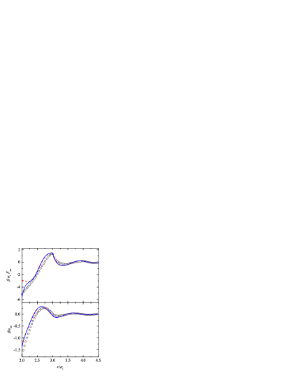
Figure 1: (Color online) Depletion force and depletion potential between two identical (big) hard spheres embedded into a solvent bath of (small) hard spheres as functions of distance. In this case, $\Sigma=1$, $R=2$, and $\eta=0.3$. Solid line: RFA approach; dashed line: PY result; circles: simulation data from Ref. AL01, .

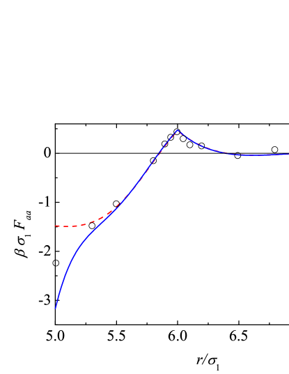
Figure 2: (Color online) Depletion force between two identical (big) hard spheres embedded into a solvent bath of (small) hard spheres as a function of distance. In this case, $\Sigma=1$, $R=5$, and $\eta=0.116$. Solid line: RFA approach; dashed line: PY result; circles: simulation data from Ref. DAS97, .

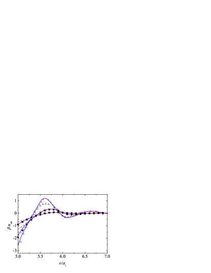
Figure 3: (Color online) Depletion potential between two identical (big) hard spheres embedded into a solvent bath of (small) hard spheres as a function of distance. In this case, $\Sigma=1$, $R=5$, and results are displayed for three values of $\eta$. Solid lines: RFA approach; dashed lines: PY results; squares: simulation data for $\eta=0.1$ from Refs. MK07, (open symbols) and LM04, (filled symbols); circles: simulation data for $\eta=0.2$ from Refs. MK07, (open symbols) and LM04, (filled symbols); triangles: simulation data for $\eta=0.3$ from Ref. LM04, .

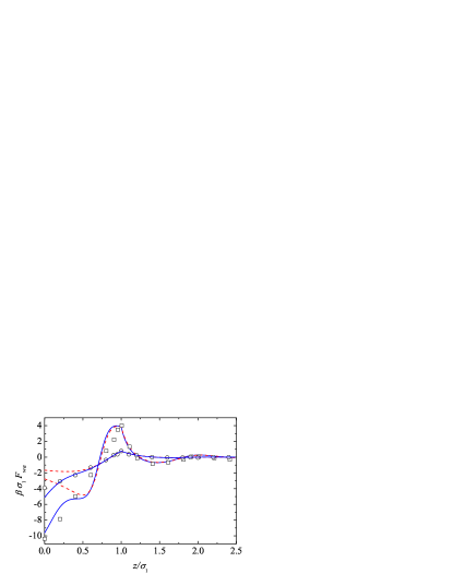
Figure 4: (Color online) Depletion force between a hard planar wall and a (big) sphere in a background fluid of (small) hard spheres. In this case, $\Sigma\to\infty$, $R=5$, and results are displayed for two values of $\eta$. Solid line: RFA approach; dashed line: PY result; circles: simulation data for $\eta=0.1$ from Ref. DAS97, ; squares: simulation data for $\eta=0.2$ from Ref. DAS97, .

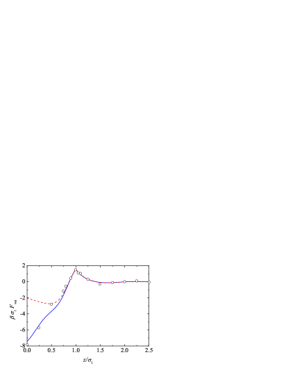
Figure 5: (Color online) Depletion force between a hard planar wall and a (big) sphere in a background fluid of (small) hard spheres. In this case, $\Sigma\to\infty$, $R=10$, and $\eta=0.1$. Solid line: RFA approach; dashed line: PY result; circles: simulation data from Ref. DAS97,

As can be seen from the figures, the RFA results certainly represent an improvement over the PY theory in all cases for both the depletion force and the depletion potential, yielding in particular much better values for the well depth in the depletion potential. Our analysis will begin with the cases where both solute particles have the same size ($\Sigma=1$), namely those in Figs. 1–3. The RFA results are clearly superior to the PY ones in the region $\sigma_{a}\leq r\lesssim\sigma_{a}+\frac{1}{2}\sigma_{1}$. For larger distances, however, the RFA and PY predictions are hardly distinguishable. When $R=2$ (see Fig. 1) the oscillations of both the RFA and the PY curves are slightly dephased with respect to the simulation data. A similar behavior is exhibited by the density functional theory shown in Fig. 2a of Ref. AL01, . Figure 1 also shows that the depletion force is a much more stringent quantity than the depletion potential. In particular, the PY theory predicts a local minimum of $F_{aa}$ (associated with an inflection point of $u_{aa}$) at $r\simeq\sigma_{a}+0.2\sigma_{1}$, while both the RFA and the simulation data present a monotonic increase of $F_{aa}$ in the region $\sigma_{a}\leq r\leq\sigma_{a}+\sigma_{1}$. If $R=5$ (Figs. 2 and 3), we observe a good performance of the RFA for the depletion force at $\eta=0.116$ (Fig. 2), except near contact. On the other hand, the theory is able to capture even quantitatively all the features of the depletion potential for $\eta=0.1$ and $\eta=0.2$ (Fig. 3). For $\eta=0.3$, paradoxically in contrast to the case $R=2$ of Fig. 1, it follows correctly the trend of the oscillations but otherwise overestimates the barrier height. Although not shown here and most likely related with the previous deficiency, also for $\eta=0.3$ the force starts to present features that seem not to occur in the simulations. We will come back to this point later on in connection with the hard planar wall limit $\Sigma\to\infty$.

Now we turn to a more stringent situation, namely the case where the depletion effect takes place between a hard planar wall and a solute sphere, i.e., $\Sigma\to\infty$. In this instance, as shown in Figs. 4 and 5, the agreement between the RFA results and the simulation data is also reasonably good. Particularly rewarding is the fact that, at least for $\eta=0.1$, one gets a good performance even when $R=10$ (Fig. 5). Analogously to the cases with $\Sigma=1$, the RFA strongly improves over the PY results for distances $z\lesssim\frac{3}{4}\sigma_{1}$ from the wall but both theories practically coincide for larger distances. Also, the PY theory predicts a spurious local minimum of the depletion force near $z=\frac{1}{2}\sigma_{1}$. It should be pointed out that in the planar wall limit one also starts to get a peculiar behavior, not shown in the figures, for relatively low densities ($\eta=0.2$ if $R=10$). This behavior, also shared by the PY theory, has similar features to the ones mentioned in connection with the poorer performance for some systems having $\Sigma=1$, that is, the appearance of spurious local minima in the depletion forces and of inflection points in the depletion potentials. While in the case $\Sigma=1$ within the RFA approach they may have their origin on the decreasing reliability of the contact values of the radial distribution functions with increasing size disparity $R$, when $\Sigma\to\infty$ the features have to do with the fact that in the hard planar wall limit the radial distribution functions both for the PY theory and in the RFA may become negative around the first minimum, MYSL07 which is clearly unphysical.

V Discussion

In this paper we have derived the depletion force and potential between two (in principle different in size) large spheres whose interaction is mediated by the presence of a multicomponent hard-sphere mixture (the solvent) composed of smaller particles. This has been done by using the RFA approach and the end results turn out to be completely analytical in Laplace space. One may say that the RFA approach not only retains the analytical character of the PY theory and the good performance of this latter at long distances, but it has some further assets as well. Hence, apart from the elimination of the thermodynamic consistency problem, it is also able to correct the main drawbacks in the PY formulation in connection with the present problem, namely the poor prediction of the short distance behavior and of the well depth in the depletion potential and the non-divergent character of the stickiness parameter in the colloidal limit. Since it seems natural that the most relevant part of the depletion potential be the one corresponding to short distances, the improvement over the PY result in this particular region may be considered as a success of the RFA approach. But the fact that after such an improvement one can also cater for the (correct) long and intermediate distance behaviors represents another nice feature of the approach. It should be clear that, while for simplicity in the illustrative examples we have considered that the solvent is a monocomponent fluid, our development is far more general allowing us in principle to examine the same problem but with the solvent being a polydisperse hard-sphere mixture.HWT03 As far as we know, no simulation data for such a system are available and so a comparison in this instance is not possible yet. In general, our expectation that the RFA produces reasonably accurate results both for the depletion forces and the depletion potential for low and moderate densities, provided the solute-solvent size ratio $R$ is not too big, is fulfilled.

We have already pointed out one of the limitations of the RFA approach (also present in the PY theory), namely the fact that in extreme conditions it may lead to unphysical (negative) values for the distribution function $\gamma_{wa}(z)$, which in turn yield spurious features in the depletion interaction $u_{wa}(z)$. One technical point must be mentioned at this stage. It concerns the choice of contact values for the radial distribution functions of the mixture and the isothermal susceptibility. While here we have considered the eCSK3 contact values [see Eq. (LABEL:eCSK3)] and an isothermal compressibility $\chi$ that is thermodynamically consistent [see Eq. (23)], the RFA approach does not forbid the possibility of other choices. For instance, for high values of $R$ one could instead take the simulation results or the ad hoc proposal of Henderson and ChanHC97 for the contact value $\gamma_{wa}(0)$. However, we have checked that, when using the empirical $\gamma_{wa}(0)$, the region where $\gamma_{wa}(z)$ takes negative values does not disappear, although those values become less negative. We would expect of course that the more accurate the contact values of the radial distribution functions and the isothermal susceptibility we use as an input, the better the performance of our development. This, however, remains to be assessed.

Finally, we want to point out that in this paper we have restricted ourselves to the infinite dilution limit of the two solute particles. This has allowed us to equate the depletion potential with the potential of mean force. If the concentration of the solute is increased, this approximation will cease to be valid. An important asset of the RFA is that it also yields analytical expressions for the direct correlation functions and the bridge functions of the mixture. These expressions could in principle be used for finite concentrations of the solute, for instance following the formulation of the depletion potential made by Castañeda-Priego et al.CRM06 This we plan to do in future work.

Appendix A Derivation of the exact low density behavior of $g_{ij}(r)$

In a general mixture, the cavity function corresponding to the pair $ij$ is defined as $y_{ij}(r)\equiv e^{\beta\phi_{ij}(r)}g_{ij}(r)$, where $\phi_{ij}(r)$ is the interaction potential. To first order in density,

$$y_{ij}(r)=1+\rho y_{ij}^{(1)}(r)+\mathcal{O}(\rho^{2}),\quad y_{ij}^{(1)}(r)=\sum_{k}x_{k}y_{ij;k}^{(1)}(r),$$ (50)

where

$$y_{ij;k}^{(1)}(r)=\int d\mathbf{r}^{\prime}\,f_{ik}(r^{\prime})f_{jk}(|\mathbf{r}-\mathbf{r}^{\prime}|),$$ (51)

$f_{ij}(r)\equiv e^{-\beta\phi_{ij}(r)}-1$ being the Mayer function. In the case of hard spheres, $f_{ij}(r)=-\Theta(r-\sigma_{ij})$, so that

$$y_{ij;k}^{(1)}(r)=V(\sigma_{ik},\sigma_{kj};r),$$ (52)

$$g_{ij;k}^{(1)}(r)=V(\sigma_{ik},\sigma_{kj};r)\Theta(r-\sigma_{ij}),$$ (53)

where $V(R_{1},R_{2};r)$ denotes the intersection volume of two spheres of radii $R_{1}$ and $R_{2}$ whose centers are a distance $r\leq R_{1}+R_{2}$ apart. If $r<R_{1}-R_{2}$ (where, without loss of generality, we have assumed that $R_{1}\geq R_{2}$) the small sphere is entirely contained inside the large one, so that the intersection volume is just the volume of the small sphere, i.e., $V(R_{1},R_{2};r)=\frac{4\pi}{3}R_{2}^{3}$. On the other hand, if $r>R_{1}-R_{2}$, the intersection volume is the sum of the volumes of two spherical caps of heights $h_{1}$ and $h_{2}$, respectively, i.e., $V(R_{1},R_{2};r)=v(R_{1};h_{1})+v(R_{2};h_{2})$, where we have denoted by $v(R;h)$ the volume of a spherical cap of height $h$ in a sphere of radius $R$. Its expression is

$$v(R;h)=\frac{\pi}{3}h^{2}(3R-h).$$ (54)

It remains to obtain $h_{1}$ and $h_{2}$ in terms of $R_{1}$, $R_{2}$, and $r$. A simple geometrical construction shows that

$$h_{1}+h_{2}=R_{1}+R_{2}-r,\quad R_{1}^{2}-(R_{1}-h_{1})^{2}=R_{2}^{2}-(R_{2}-h_{2})^{2},$$ (55)

whose solution is

$$h_{1}=\frac{(R_{1}+R_{2}-r)(R_{2}-R_{1}+r)}{2r},\quad h_{2}=\frac{(R_{1}+R_{2}-r)(R_{1}-R_{2}+r)}{2r}.$$ (56)

The final result is then

$$V(R_{1},R_{2};r)=\begin{cases}\frac{4\pi}{3}R_{2}^{3},&r<R_{1}-R_{2},\\ \frac{\pi}{12r}(R_{1}+R_{2}-r)^{2}[r^{2}+2(R_{1}+R_{2})r-3(R_{1}-R_{2})^{2}],&R_{1}-R_{2}<r<R_{1}+R_{2},\\ 0,&r>R_{1}+R_{2}.\end{cases}$$ (57)

Equation (4) follows from Eqs. (53) and (57), where it is assumed that $\sigma_{ij}\leq\sigma_{ik}+\sigma_{kj}$ for all sets $\{i,j,k\}$.

Appendix B Effective stickiness of the depletion potential

The second virial coefficient associated with the depletion potential $u_{aa}(r)$ is

$$B_{2} = -{2\pi}\int_{0}^{\infty}dr\,r^{2}\left[e^{-\beta u_{aa}(r)}-1\right]$$ (58)

$$= \frac{2\pi}{3}\sigma_{a}^{3}\left\{1-\frac{3}{\sigma_{a}^{3}}\int_{\sigma_{a}}^{\infty}dr\,r^{2}\left[g_{aa}(r)-1\right]\right\}.$$

From here one can define the “stickiness” parameterNF00

$$\tau^{-1} = 4-\frac{6B_{2}}{\pi\sigma_{a}^{3}}$$ (59)

$$= -\frac{12}{\sigma_{a}^{3}}\frac{\partial}{\partial s}\left[G_{aa}(s)-e^{-\sigma_{a}s}\frac{1+\sigma_{a}s}{s^{2}}\right]_{s=0}.$$

Making use of Eq. (36) one gets an explicit expression of $\tau^{-1}$ in terms of the packing fraction $\eta$, the size ratio $\sigma_{a}/\sigma_{1}$, the RFA parameter $\alpha$, and the imposed contact values $g_{aa}(\sigma_{a})$, $g_{a1}(\sigma_{a1})$, and $g_{11}(\sigma_{1})$. In the special case of the PY approximation ($\alpha=0$), the result is

$$\tau^{-1} = \frac{\eta}{2(1+2\eta)^{2}}\left[12(1+2\eta)+3(5+4\eta)\sigma_{1}/\sigma_{a}\right.$$ (60)

$$\left.+6(1-\eta)(\sigma_{1}/\sigma_{a})^{2}+(1-\eta)^{2}(\sigma_{1}/\sigma_{a})^{3}\right].$$

In this approximation, the stickiness parameter $\tau^{-1}$ is lower bounded by

$$\tau_{\text{coll}}^{-1}=\frac{6\eta}{1+2\eta}.$$ (61)

In fact, this lower bound is the value in the colloidal limit $\sigma_{a}/\sigma_{1}\to\infty$. Moreover, the PY contact values in the colloidal limit are

$$g_{aa}(\sigma_{a}) = \frac{\sigma_{a}}{\sigma_{1}}\frac{3\eta}{2(1-\eta)^{2}},$$

$$g_{a1}(\sigma_{a1}) = \frac{1+2\eta}{(1-\eta)^{2}},$$ (62)

$$g_{11}(\sigma_{1}) = \frac{1+\eta/2}{(1-\eta)^{2}}.$$

In contrast to Eq. (61), the stickiness parameter predicted by the RFA ($\alpha\neq 0$) in the colloidal limit becomes

$$\tau_{\text{coll}}^{-1}=12(\sigma_{1}/\sigma_{a}){\alpha^{*}}g_{aa}(\sigma_{aa})+6\eta\frac{1+3{\alpha^{*}}[1-2g_{a1}(\sigma_{a1})+2\eta g_{11}(\sigma_{1})]-6{\alpha^{*}}^{2}g_{a1}(\sigma_{a1})\left[1-(1-\eta)g_{a1}(\sigma_{a1})\right]}{1+2\eta+6{\alpha^{*}}\eta\left[1-2(1-\eta)g_{11}(\sigma_{1})\right]},$$ (63)

where $\alpha^{*}\equiv\alpha/\sigma_{1}$. Equation (63) implies that, unless $g_{aa}(\sigma_{a})\sim(\sigma_{a}/\sigma_{1})$, the stickiness parameter diverges in the colloidal limit, i.e.

$$\tau_{\text{coll}}^{-1}=12(\sigma_{1}/\sigma_{a}){\alpha^{*}}g_{aa}(\sigma_{a}).$$ (64)

The behavior $g_{aa}(\sigma_{a})\sim(\sigma_{a}/\sigma_{1})$ appears in the PY theory. However, other theories (like the SPT, the BGHLL, and the one proposed by us in Ref. SYH99, ) assume that $g_{aa}(\sigma_{a})\sim(\sigma_{a}/\sigma_{1})^{2}$, while $g_{aa}(\sigma_{a})\sim(\sigma_{a}/\sigma_{1})^{3}$ in our recent proposalSYH05 and $\ln g_{aa}(\sigma_{a})\sim(\sigma_{a}/\sigma_{1})$ according to Henderson and Chan.HC97 A simple geometrical argument shows that the divergence of $\tau^{-1}$ in the colloidal limit is not an artifact of the RFA. The parameter $\tau^{-1}$ essentially measures the area (in units of $\sigma_{a}^{3}$) below the curve $r^{2}[g_{aa}(r)-1]$ between $r=\sigma_{a}$ and $r\to\infty$. For large $\sigma_{a}/\sigma_{1}$ the range of $g_{aa}(r)-1$ is expected to be of the order of $\sigma_{1}$. Therefore, the area can be estimated as

$$\tau_{\text{coll}}^{-1}\sim\frac{1}{\sigma_{a}^{3}}\sigma_{a}^{2}[g_{aa}(\sigma_{a})-1]\sigma_{1}\sim\frac{\sigma_{1}}{\sigma_{a}}g_{aa}(\sigma_{a}),$$ (65)

in agreement with the leading term in Eq. (63). To refine that argument, let us define the range $\xi$ of $r^{2}[g_{aa}(r)-1]$ as

$$\xi^{-1} = -\left.\frac{\partial}{\partial r}\ln\left[r^{2}g_{aa}(r)\right]\right|_{r=\sigma_{a}}$$ (66)

$$= -\frac{g_{aa}^{\prime}(\sigma_{a})}{g_{aa}(\sigma_{a})}-\frac{2}{\sigma_{a}}.$$

Taking into account the definition of $G_{aa}(s)$ as the Laplace transform of $rg_{aa}(r)$, we have

$$\xi^{-1}=-\frac{1}{\sigma_{a}}-\lim_{s\to\infty}s\left[\frac{se^{\sigma_{a}s}G_{aa}(s)}{\sigma_{a}g_{aa}(\sigma_{a})}-1\right].$$ (67)

In the PY approximation, the result is

$$\xi_{\text{coll}}=\sigma_{1}\frac{1-\eta}{2(1+2\eta)}$$ (68)

in the colloidal limit. On the other hand, the RFA yields in that limit

$$\xi_{\text{coll}} = \sigma_{1}\left\{\frac{g_{a1}(\sigma_{a1})}{g_{aa}(\sigma_{a})}\frac{\sigma_{a}}{\sigma_{1}}\frac{3\eta}{1-\eta}\right.$$ (69)

$$\left.+\frac{1}{\alpha^{*}}\left[1-\frac{\sigma_{a}}{\sigma_{1}}\frac{3\eta}{2(1-\eta)g_{aa}(\sigma_{a})}\right]\right\}^{-1}.$$

If $g_{aa}$ diverges more rapidly than $\sigma_{a}/\sigma_{1}$, we get

$$\xi_{\text{coll}}=\alpha^{*}\sigma_{1}=\alpha,$$ (70)

which is generally much shorter than the PY result. In general, we have

$$\tau_{\text{coll}}^{-1}=12\mu\frac{g_{aa}(\sigma_{a})}{\sigma_{a}}\xi_{\text{coll}},$$ (71)

where $\mu$ is of the order of 1. In the PY approximation we get $\mu=1/3(1-\eta)$, while $\mu=1$ in the RFA.

References

• (1) S. Asakura and F. Oosawa, J. Chem. Phys. 22, 1255 (1954); J. Polym. Sci. 33, 183 (1958).
• (2) A. G. Yodh, K.-H. Lin, J. C. Crocker, A. D. Dinsmore, R. Verma, and P. D. Kaplan, Phil. Trans. R. Soc. Lond. A 359, 921 (2001).
• (3) B. Götzelmann, R. Evans, and S. Dietrich, Phys. Rev. E 57, 6785 (1998).
• (4) B. Götzelmann, R. Roth, S. Dietrich, M. Dijkstra, and R. Evans, Europhys. Lett. 47, 398 (1999).
• (5) C. Bechinger, D. Rudhart, P. Leiderer, R. Roth, and S. Dietrich, Phys. Rev. Lett. 83, 3960 (1999).
• (6) R. Roth, R. Evans, and S. Dietrich, Phys. Rev. E 62, 5360 (2000).
• (7) S. Amokrane, A. Ayadim, and J. G. Malherbe, J. Phys.: Condens. Matter 15, S3443 (2003).
• (8) D. Zhu, W. Li, and H. R. Ma, J. Phys.: Condens. Matter 15, 8281 (2003).
• (9) W. Li and H. R. Ma, Chin. Phys. Lett. 21, 1175 (2004).
• (10) R. Roth and P.-M. König, Pramana 64, 971 (2005).
• (11) T. Biben, P. Bladon, and D. Frenkel, J. Phys.: Condens. Matter 8, 10799 (1996).
• (12) R. Dickman, P. Attard, and V. Simonian, J. Chem. Phys. 107, 205 (1997).
• (13) M. Dijkstra, R. van Roij, and R. Evans, Phys. Rev. Lett. 82, 117 (1999).
• (14) E. Allahyarov and H. Löwen, Phys. Rev. E 63, 041403 (2001).
• (15) W. Li, S. Xue, and H. R. Ma, Journal of Shanghai Jiaotong University, E-6, 126 (2001).
• (16) A. R. Herring and J. R. Henderson, Phys. Rev. Lett. 97, 148302 (2006).
• (17) J. G. Malherbe and W. Krauth, Mol. Phys. (2007) (in press); arXiv:0705.4168 [cond-mat.soft].
• (18) Y. Mao, M. E. Cates, and H. N. W. Lekkerkerker, Physica A 222, 10 (1995).
• (19) J. R. Henderson, Physica A 313, 321 (2002).
• (20) S. M. Oversteegen and H. N. W. Lekkerkerker, Physica A 341, 23 (2004).
• (21) M. Oettel, Phys. Rev. E 69, 041404 (2004).
• (22) A. R. Herring and J. R. Henderson, Phys. Rev. E 75, 011402 (2007).
• (23) D. Henderson and M. Lozada-Cassou, J. Colloid Interface Sci. 114, 180 (1986).
• (24) D. Henderson, J. Colloid Interface Sci. 121, 486 (1988).
• (25) P. Attard and G. N. Patey, J. Chem. Phys. 92, 4970 (1990).
• (26) D. Henderson, J. Chem. Phys. 97, 1266 (1992).
• (27) J. M. Méndez-Alcaraz and R. Klein, Phys. Rev. E 61, 4095 (2000).
• (28) D. Henderson, D. T. Wasan, and A. Trokhymchuk, Condensed Matter Physics 4, 779 (2001).
• (29) J. A. Anta and S. Lago, J. Chem. Phys. 116, 10514 (2002).
• (30) D. Henderson, D. T. Wasan, and A. Trokhymchuk, J. Chem. Phys. 119, 11989 (2003).
• (31) R. Castañeda-Priego, A. Rodríguez-López, and J. M. Méndez-Alcaraz, J. Phys.: Condens. Matter 15, S3393 (2003).
• (32) Ph. Germain, J. G. Malherbe, and S. Amokrane, Phys. Rev. E 70, 041409 (2004).
• (33) A. Ayadim, J. G. Malherbe, and S. Amokrane, J. Chem. Phys. 122, 234908 (2005).
• (34) R. Castañeda-Priego, A. Rodríguez-López, and J. M. Méndez-Alcaraz, Phys. Rev. E 73, 051404 (2006).
• (35) Al. Malijevský, S. B. Yuste, A. Santos, and M. López de Haro, Phys. Rev. E 75, 061201 (2007).
• (36) S. B. Yuste, A. Santos, and M. López de Haro, J. Chem. Phys. 108, 3683 (1998).
• (37) M. López de Haro, S.B. Yuste, and A. Santos, “Alternative Approaches to the Equilibrium Properties of Hard-Sphere Liquids,” in Playing with Marbles: Theory and Simulation of Hard-Sphere Fluids and Related Systems, edited by A. Mulero (Springer, Berlin, to be published); preprint arXiv:0704.0157 [cond-mat.stat-mech].
• (38) J. L. Lebowitz, Phys. Rev. 133, 895 (1964).
• (39) L. Blum and J. S. Høye, J. Phys. Chem. 81, 1311 (1977).
• (40) A. Santos, S. B. Yuste, and M. López de Haro, J. Chem. Phys. 123, 234512 (2005); M. López de Haro, S. B. Yuste, and A. Santos, Mol. Phys. 104, 3461 (2006).
• (41) T. Boublík, Mol. Phys. 59, 371 (1986).
• (42) D. Henderson and K.-Y. Chan, Mol. Phys. 91, 1137 (1997); J. Chem. Phys. 108, 9946 (1998).
• (43) M. Noro and D. Frenkel, J. Chem.Phys. 113, 2941 (2000).
• (44) A. Santos, S. B. Yuste, and M. López de Haro, Mol. Phys. 96, 1 (1999).