Prior-predictive value from fast growth simulations

Abstract

Building on a variant of the Jarzynski equation we propose a new method to numerically determine the prior-predictive value in a Bayesian inference problem. The method generalizes thermodynamic integration and is not hampered by equilibration problems. We demonstrate its operation by applying it to two simple examples and elucidate its performance. In the case of multi-modal posterior distributions the performance is superior to thermodynamic integration.

I Introduction

Bayesian methods of inference Jaynes ; GCSR ; LeHs are playing an ever growing role in the statistical analysis of data in physics and other natural sciences BBDS ; Agostini ; Doserev . Among its particular virtues is the ability to perform model selection, i.e. to quantitatively assess the appropriateness of a particular model irrespective of concrete parameter values. This is accomplished by calculating what is called the evidence or the prior-predictive value.

Building on rather general and essentially simple principles the efficiency of Bayesian methods in practical applications depends crucially on the implemented numerical algorithms. A major difficulty common to Bayesian data analysis is the calculation of integrals in high-dimensional spaces which are dominated by contributions from small and labyrinthine regions. Similar problems are typical for the numerical determination of the partition function in statistical mechanics. It is therefore no surprise that some of the tools developed in statistical mechanics have found their way into the arsenal of methods used in Bayesian inference.

In the present paper we show that recent progress in the statistical mechanics of non-equilibrium processes Jar ; JarFT ; Crooks ; Seifert entails new possibilities to estimate the prior-predictive value and to average with the posterior distribution of a Bayesian analysis. The new method relies on the Monte-Carlo (MC) simulation of a non-stationary Markov process and is intermediate between straight MC sampling and thermodynamic integration thdint . It is generally superior to the first and may also outperform the second. We first give a general theoretical discussion and then analyze numerically two simple examples. One of these was used already in LPD to scrutinize the efficiency of thermodynamic integration. The second is a generalization thereof employing a bimodal likelihood.

II Theory

We consider a standard Bayesian inference problem in which parameters $x$ of a model ${\cal M}$ are to be determined from data $d$. The prior information about $x$ is coded in a prior distribution $p_{p}(x|{\cal M})$, the likelihood of the data given certain values of $x$ is denoted by $p_{l}(d|x,{\cal M})$. By Bayes’ theorem the posterior distribution is given by

$$p_{\mathrm{post}}(x|d,{\cal M})=\frac{p_{l}(d|x,{\cal M})\,p_{p}(x|{\cal M})}{P(d|{\cal M})}\,.$$ (1)

Our central quantity of interest is the normalization of the posterior, the so called evidence or prior-predictive value, defined by

$$P(d|{\cal M})=\int dx\,p_{l}(d|x,{\cal M})\,p_{p}(x|{\cal M})\,.$$ (2)

It quantifies the likeliness of the data for the particular model ${\cal M}$ under consideration and is therefore crucial for the comparison between different models. For the following manipulations the dependence of $p_{p}(x|{\cal M})$ and $p_{l}(d|x,{\cal M})$ on $x$ will be the important one, in order to lighten the notation we will therefore suppress the dependencies on $d$ and ${\cal M}$ in these quantities. Generically the integral in (2) is dominated by intricately shaped regions in a high-dimensional space and is therefore difficult to determine.

A possible remedy for this problem is motivated by the method of thermodynamic integration used in statistical mechanics. To this end one introduces the auxiliary quantity

$$Z(\beta):=\int dx\,\big{(}p_{l}(x)\big{)}^{\beta}p_{p}(x)\,.$$ (3)

Clearly $Z(0)=1$ due to the normalization of the prior distribution and $Z(1)=P(d|{\cal M})$, the desired quantity. Moreover

$$\frac{\partial}{\partial\beta}\ln Z(\beta) =\frac{1}{Z(\beta)}\int dx\ln p_{l}(x)\;p_{l}^{\beta}(x)\,p_{p}(x)$$

$$=:\langle\ln p_{l}(x)\rangle_{\beta}\,,$$

where the $\beta$-average in the last line is taken with the distribution

$$P_{\beta}(x):=\frac{1}{Z(\beta)}\;p_{l}^{\beta}(x)\,p_{p}(x)\,.$$ (4)

We therefore get

$$\ln P(d|{\cal M})=\int_{0}^{1}d\beta\,\frac{\partial}{\partial\beta}\ln Z(\beta)=\int_{0}^{1}d\beta\,\langle\ln p_{l}(x)\rangle_{\beta}\,,$$ (5)

from which the name thermodynamic integration for the method becomes clear.

Since averages are much more efficiently calculated from MC simulations than normalization factors (5) offers a convenient way to determine $P(d|{\cal M})$ from equilibrium simulations for just a few values of $\beta$ between 0 and 1. The method was suggested in thdint , its advantages over a straight-forward MC estimation of $P(d|{\cal M})$ from (2) was demonstrated for a simple test example in LPD .

Let us consider the MC simulations necessary to implement (5) in somewhat more detail. We first discretize the $\beta$-interval by introducing $M$ values $\beta_{m},m=1,...,M$, with $0=\beta_{1}<\beta_{2}<...<\beta_{M}=1$. For each $\beta_{m}$ we generate a trajectory $x_{t}$ with a discrete time $t=1,2,...$ measured in MC steps. These trajectories are realizations of a Markov process with transition probability $\rho(x,x^{\prime};\beta_{m})$ which leaves the distribution defined in (4) invariant, i.e. which satisfies

$$P_{\beta_{m}}(x)=\int dx^{\prime}\rho(x,x^{\prime};\beta_{m})P_{\beta_{m}}(x^{\prime})\,.$$ (6)

A sufficiently long Markov chain is now generated for each $\beta_{m}$ in order to get a reliable estimate for $\langle\ln p_{l}(x)\rangle_{\beta}$ to be used in (5). This equilibration of the system at each value of $\beta$ is the main bottleneck of the method. In realistic situations with a multi-modal or otherwise complicated structure of the likelihood it may become very slow and special care must be taken which elements of the trajectory $x_{t}$ to use for the estimation of the average $\langle\ln p_{l}(x)\rangle_{\beta}$. As a rule specific quantities need to be identified and monitored which indicate when the system has approximately equilibrated.

These equilibration problems may be avoided by building on recent progress in the statistical mechanics of non-equilibrium processes Jar ; JarFT ; Crooks ; Seifert ; LeSp ; Chatelain . In the present context it gives rise to the following procedure to determine $Z(1)$. We fix a time interval $t=1,...,N$ and generate a set of trajectories $x_{t}$ from a non-stationary Markov process such that for each trajectory $\beta$ changes from 0 to 1. More precisely we fix $M\leq N$ intermediate time points $t_{m},m=1,...,M$ with $1\leq t_{1}<t_{2}<....<t_{M}\leq N$ at which $\beta$ changes by $\Delta\beta_{m}=\beta_{m+1}-\beta_{m}$. We call the set $\{\Delta\beta_{m},t_{m}\}$ of these time points and the corresponding increments in $\beta$ the protocol of the procedure.

Consider a trajectory $\{x_{t}\}$ that starts in $x_{1}$ drawn from the prior distribution $p_{p}$ and then evolves according to $\rho(x,x^{\prime};\beta_{m})$ with $\beta_{m}$ fixed by the protocol $\{\Delta\beta_{m},t_{m}\}$. The probability $\mathcal{P}(\{x_{t}\})$ of the whole trajectory is given by

$$\mathcal{P}(\{x_{t}\})=p_{p}(x_{1})\prod_{t=1}^{N-1}\rho(x_{t+1},x_{t};\beta_{m})\,.$$ (7)

Consider now the trajectory dependent functional

$$R(\{x_{t}\})=\sum_{m=1}^{M-1}\Delta\beta_{m}\,\ln p_{l}(x_{t_{m}})\,,$$ (8)

which is a random quantity due to its dependence on $\{x_{t}\}$. We will show that its exponential average

$$\langle e^{R}\rangle= \int\prod_{t=1}^{N}dx_{t}\;\mathcal{P}(\{x_{t}\})\;e^{R(\{x_{t}\})}$$

$$= \int\!\!\prod_{t=1}^{N}dx_{t}\;p_{p}(x_{1})\!\!\prod_{t=1}^{N-1}\rho(x_{t+1},x_{t};\beta_{m})\!\!\prod_{m=1}^{M-1}\Big{(}p_{l}(x_{t_{m}})\Big{)}^{\Delta\beta_{m}}$$

is equal to the desired quantity $Z(1)=P(d|{\cal M})$.

To this end we first note that the integrations over the first $x_{t}$ with $1\leq t<t_{1}$ are easily performed since during these time steps $\beta=\beta_{1}=0$. Using (6) repeatedly for $\beta=0$ we find

$$\int\prod_{t=1}^{t_{1}-1}dx_{t}\;p_{p}(x_{1})\prod_{t=1}^{t_{1}-1}\rho(x_{t+1},x_{t};0)=p_{p}(x_{t_{1}})\,.$$ (9)

Together with the $m=1$ term in (8) and using (4) as well as $\Delta\beta_{1}=\beta_{2}$ we hence obtain

$$\int\prod_{t=1}^{t_{1}-1} dx_{t}\;p_{p}(x_{1})\prod_{t=1}^{t_{1}-1}\rho(x_{t+1},x_{t};0)\exp\big{(}\Delta\beta_{1}\,\ln p_{l}(x_{t_{1}})\big{)}$$

$$=p_{p}(x_{t_{1}})\,p_{l}^{\beta_{2}}(x_{t_{1}})$$

$$=Z(\beta_{2})\,P_{\beta_{2}}(x_{t_{1}})\,.$$

The integrations over the $x_{t}$ with $t_{1}\leq t<t_{2}$ can now be performed analogously. According to (6) we get at first

$$\int\prod_{t=t_{1}}^{t_{2}-1}dx_{t}\;P_{\beta_{2}}(x_{t_{1}})\prod_{t=t_{1}}^{t_{2}-1}\rho(x_{t+1},x_{t};\beta_{2})=P_{\beta_{2}}(x_{t_{2}})\,.$$ (10)

since $\beta=\beta_{2}$ for the whole interval. Together with the second term of the sum in (8) we hence have

$$Z(\beta_{2}) \,P_{\beta_{2}}(x_{t_{2}})\,\exp\big{(}\Delta\beta_{2}\ln p_{l}(x_{t_{2}})\big{)}$$

$$=p_{p}(x_{t_{2}})\;p_{l}^{\beta_{2}}(x_{t_{2}})\;p_{l}^{\beta_{3}-\beta_{2}}(x_{t_{2}})$$

$$=p_{p}(x_{t_{2}})\;p_{l}^{\beta_{3}}(x_{t_{2}})$$

$$=Z(\beta_{3})\,P_{\beta_{3}}(x_{t_{2}})\,.$$

Iterating this procedure we finally arrive at

$$\langle e^{R}\rangle=Z(\beta_{M})\int dx_{N}P_{\beta_{M}}(x_{N})=Z(1)=P(d|{\cal M})\,.$$ (11)

Generalizing this relation to continuous protocols $\beta(t)$ with $0\leq t\leq t_{f}$ we obtain

$$P(d|{\cal M})=\left\langle\exp\big{(}\int_{0}^{t_{f}}dt\ln p_{l}(x(t))\;\frac{\partial}{\partial t}\beta(t)\big{)}\right\rangle\,.$$ (12)

Eqs. (11) and (12) are our central result. The prior-predictive value can be determined from an exponential average of the quantity $R(\{x_{t}\})$ defined in (8) over an ensemble of MC trajectories $x_{t}$ generated with a transition probability $\rho(x,x^{\prime};\beta(t))$ that depends explicitly on time via the protocol $\beta(t)$. Note that this protocol must be the same for all trajectories $\{x_{t}\}$ that are used to determine the average $\langle e^{R}\rangle$. It is nevertheless very remarkable that the results (11) and (12) respectively do not depend on the details of this protocol.

As a small aside we note that in a Bayesian analysis one is usually more interested in averages with the posterior distribution (1) than in this distribution itself. By a slight generalization of the above proof one can show for the posterior average of some function $f(x)$

$$\langle f\rangle_{\mathrm{post}} =\int dxf(x)p_{\mathrm{post}}(x)=\int dx_{N}f(x_{N})P_{\beta=1}(x_{N})$$

$$=\frac{\langle e^{R}f(x_{N})\rangle}{\langle e^{R}\rangle}\,,$$ (13)

where the averages in the last line are taken with $\mathcal{P}(\{x_{t}\})$. Posterior averages may hence be determined from path averages starting from the prior distribution and incorporating the weight factor $e^{R}$, cf. Crooks for an analogous result in the statistical mechanics framework.

Two limiting cases of Eqs. (11) and (12) are of interest. For $1\ll M$ the system is manipulated in quasi-equilibrium and $\beta$ and thus $P_{\beta}(x)$ change very slowly. Accordingly the Markov chain will explore much of the state space for a given small $\beta$-interval and we may therefore replace $\ln p_{l}(x_{t_{m}})$ in (8) by $\langle\ln p_{l}(x)\rangle_{\beta_{m}}$. As a consequence $R$ no longer depends on the individual realizations of the trajectories $\{x_{t}\}$ and the average in (12) becomes superfluous. Therefore

$$P(d|{\cal M}) =\exp\big{(}\int_{0}^{t_{f}}dt\;\langle\ln p_{l}(x)\rangle_{\beta}\;\frac{\partial}{\partial t}\beta(t)\big{)}$$

$$=\exp\big{(}\int_{0}^{1}d\beta\langle\ln p_{l}(x)\rangle_{\beta}\big{)}$$ (14)

which brings us back to thermodynamic integration, cf. (5).

In the opposite limit $\beta$ is changed in a single step from zero to one at some time $t=t_{*}$, i.e. $\beta=\theta(t-t_{*})$ with the Heaviside $\theta$-function being 1 for positive arguments and zero else. In this case the time integral in (12) picks up contributions from $t=t_{*}$ only and the average over the trajectories $\{x_{t}\}$ reduces to the average over $x_{*}=x(t_{*})$ with the prior distribution $p_{p}$. We then find from (12)

$$P(d|{\cal M})=\int dx_{*}\exp(\ln p_{l}(x_{*}))\,p_{p}(x_{*})\,,$$ (15)

which is identical with (2). This limit is equivalent to what is called thermodynamic perturbation in statistical mechanics Zwanzig .

The proposed method hence interpolates between the two extreme variants (2) and (5) for the determination of the prior-predictive value $P(d|{\cal M})$. It should be superior to the straight application of (2) since the average in (12) is already shortly after the start of the trajectories influenced by the likelihood $p_{l}(x)$ which is, as a rule, much sharper than the prior. It may outperform thermodynamic integration (5) since no time-consuming equilibrations are necessary. On the other hand, the exponential average in (12) is known to be subtle. It is biased for finite sample sizes Fox ; GRB ; Hummer and dominated by rare realizations with very big values of $R$ for processes too far from equilibrium Jarzynski2 . Nevertheless, a strong argument in favour of the method is its applicability to systems that are hard to equilibrate and its great flexibility to optimization for which the whole protocol $\beta(t)$ is at our disposal.

It is also worthwhile to mention that in many situations of interest the probability distribution of $R$ is Gaussian with average $\langle R\rangle$ and variance $\sigma_{R}^{2}$ SpSe ; PaSch . In this case the average $\langle e^{R}\rangle$ can be calculated exactly with the result

$$P(d|{\cal M})=\exp\Big{(}\langle R\rangle+\frac{\sigma_{R}^{2}}{2}\Big{)}\,.$$ (16)

The determination of $\langle R\rangle$ and $\sigma_{R}^{2}$ from the MC simulations is, of course, much less demanding than the extraction of the complete distribution of $R$. For general distributions (16) gives just the first two terms of the cumulant expansion.

III Two simple examples

We now numerically investigate the performance of the method by applying it to two simple, exactly solvable examples. The first one employs a unimodal likelihood the second one uses a bimodal one. These model systems are variants of those discussed in LPD and DKEL respectively. The underlying inference problem is to estimate an $n$-dimensional vector $x$ of parameters from an $n$-dimensional vector $d$ of data with $n=128$.

For the unimodal case both prior $p_{p}(x)$ and likelihood $p_{l}^{u}(x)$ are taken to be Gaussians with zero mean and variances $\sigma_{p}^{2}$ and $\sigma_{l}^{2}$ respectively.

$$p_{l}^{u}(x) =(2\pi\sigma_{l}^{2})^{-n/2}\;\exp(-\frac{\|d-x\|^{2}}{2\sigma_{l}^{2}})$$ (17)

$$p_{p}(x) =(2\pi\sigma_{p}^{2})^{-n/2}\;\exp(-\frac{\|x\|^{2}}{2\sigma_{p}^{2}})$$ (18)

We will use $\sigma_{p}=10$ and $\sigma_{l}=1$ to model the typical situation in which the prior is substantially broader than the likelihood. Moreover we choose a data vector $d$ with

$$\bar{d}^{2}=\frac{1}{n}\sum_{i=1}^{n}d_{i}^{2}=100\;,$$ (19)

which on the one hand ensures that the data are far from the center of the prior $p_{p}(x)$, and on the other hand fixes the signal-to-noise ratio SNR$=\sqrt{\bar{d}^{2}/\sigma_{l}^{2}}$ to be 10 as in LPD . The performance of the algorithms to be discussed below does not depend on the particular values of the $d_{i}$ as long as $\bar{d}^{2}=100$ is fulfilled. We therefore use the simple prescription $d_{i}=10$ for all $i=1\ldots n$.

In the bimodal case only the likelihood differs which is given by

$$p_{l}^{b}(x)=\frac{1}{21}p_{l}^{u}(x)+\frac{20}{21}p_{l}^{u}(-x)$$ (20)

and hence consists of two Gaussians with the same variance centered at $x$ and $-x$ respectively. It is important, however, that their relative weights are markedly different from each other. Our special choice of parameters implies that in equilibrium the region around $-x$ should be sampled $20$ times as often as the one around $x$.

With the choices for prior and likelihood given above the prior-predictive value as defined in (2) can be calculated analytically. We get for both cases the result

$$P(d|\mathcal{M})=(2\pi(\sigma_{l}^{2}+\sigma_{p}^{2}))^{-n/2}\exp(-\frac{\|d\|^{2}}{2(\sigma_{l}^{2}+\sigma_{p}^{2})})\;.$$ (21)

With the parameter values chosen this yields $\ln P(d|{\cal M})=-476.358$.

In the following we will test thermodynamic integration and our procedure against the exact result. In order to present a fair comparison between the performances of the numerical methods each simulation will comprise the same number ($10^{9}$) of MC steps. This number will, however, be divided in different ways between the number $M$ of intermediate $\beta$-values, the number $N$ of MC steps per $\beta$-value for thermodynamic integration, (the number $N$ of MC steps per run for the exponential average) , and the number $N_{c}$ of runs to estimate the distribution of $R$, (to estimate the distribution of $\ln P_{\mathrm{td}}$).

The thermodynamic integration scheme (5) requires estimates of $\langle\ln p_{l}(x)\rangle_{\beta_{m}}$ at appropriately chosen values $\beta_{m}$ of $\beta$. As a rule $\langle\ln p_{l}(x)\rangle_{\beta}$ is a smooth function of $\beta$ and few such values will be sufficient. Trajectories $\{x_{t}\}$ are generated for each $\beta_{m}$ by the standard Metropolis algorithm. First a starting point $x_{1}$ is chosen at random, e.g. from the prior distribution $p_{p}$ or taken directly from the endpoints at the previous $\beta_{m}$. Subsequent moves for $t=2,...,(N-1)$ are obtained by generating a trial step $x_{t}\to x^{\prime}$ from the distribution

$$(2\pi\sigma_{\mathrm{step}}(\beta)^{2})^{-n/2}\;\exp\big{(}-\frac{\|x^{\prime}-x_{t}\|^{2}}{2\sigma_{\mathrm{step}}(\beta)^{2}}\big{)}$$ (22)

The step is accepted, $x_{t+1}=x^{\prime}$, with probability

$$p_{\mathrm{accept}}=\min[1,P_{\beta_{m}}(x^{\prime})/P_{\beta_{m}}(x_{t})]\,.$$ (23)

and rejected, $x_{t+1}=x_{t}$, otherwise. The choice $\sigma_{\mathrm{step}}(\beta)=0.25({1}/{\sigma_{p}^{2}}+{\beta}/{\sigma_{l}^{2}})^{-1/2}$ ensures a good acceptance ratio for all $\beta$ since it adapts to the width of $P_{\beta}(x)$ as given in (4). The first steps in the trajectories $\{x_{t}\}$ are not yet characteristic for the equilibrium distribution. We therefore discard the first $60\%$ of steps for equilibration. The rest is thinned out by discarding all but every tenth step to suppress correlations. From the remaining values the average $\langle\ln p_{l}(x)\rangle_{\beta}$ is determined. We then calculate $\ln P(d|{\cal M})$ by integrating a cubic spline interpolation of (5). The procedure is repeated $N_{c}$ times to obtain an average of the log prior-predictive value, $\ln P_{\mathrm{td}}$, together with an error estimate.

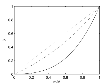
For the simulation of (12) we have first to define the protocol $\beta(t)$ according to which the parameter $\beta$ will be changed from 0 to 1. We will use three different protocols with $t_{f}=1$. Introducing $M$ equidistant time points

$$t_{m}=m\cdot\frac{t_{f}}{M}\;,\quad m=1,...,M$$

these protocols are defined respectively by (cf. fig.1)

$$\beta^{\mathrm{lin}}_{m} =\frac{m}{M}$$ (24)

$$\beta^{\mathrm{poly}}_{m} =0.05(\frac{m}{M})+0.95(\frac{m}{M})^{3}$$ (25)

$$\beta^{\mathrm{exp}}_{m} =\frac{e^{m/M}-1}{e-1}\;.$$ (26)

Figure 1: Plot of the three protocols used in the simulations. The dotted line shows the linear protocol (24), the dashed-dotted one the exponential protocol (26), and the full one the polynomial protocol defined by (25).

The trajectories $\{x_{t}\}$ are generated by the Metropolis algorithm in a similar way as in the simulation of thermodynamic integration, with, however, a few crucial differences. First, the number $M$ of intermediate $\beta$-values is much higher now. Second, $\beta$ and therefore the acceptance probability (23) changes along the trajectory. Third, the starting point $x_{1}$ must now be sampled from the prior $p_{p}(x)$. Fourth, no equilibration is necessary and hence no points will be discarded.

At each moment when $\beta$ changes a new contribution is added to $R$ according to (8). After $N_{c}$ trajectories have been simulated, a histogram of $R$-values is generated from which the average $\langle R\rangle$, the variance $\sigma_{R}$ and the exponential average $\ln\left\langle e^{R}\right\rangle$ together with an error estimate are calculated.

IV Results

IV.1 Unimodal likelihood

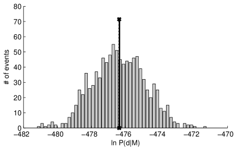
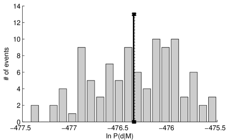
Representative results for the unimodal model from thermodynamic integration simulations are shown in figs.2 and 3 as histograms for $\ln P(d|{\cal M})$ together with their averages and the exact result (21). The intermediate values of $\beta$ where chosen according to (25) but this is not very crucial. As can be seen a very good estimate of the prior-predictive value may be obtained.

From (4) we infer that the intermediate distributions $P_{\beta}(x)$ are all Gaussians in this case and equilibration is hence no problem. This is also corroborated by the comparison between figs.2 and 3 which show that a few very long trajectories do not yield substantially better results than many long trajectories. Accordingly thermodynamic integration works well.

Figure 2: Histogram of the logarithm of the prior-predictive value for the unimodal case as obtained from thermodynamic integration using $M=100$ intermediate $\beta$-values determined according to (25), $N=10000$ MC steps per $\beta$ value and $N_{c}=1000$ runs. The dotted vertical line indicates the average $\ln P_{\mathrm{td}}=-476.386\pm 0.05$, the full one the exact result $\ln P=-476.358$.

Figure 3: Same as fig.2 with $M=20$, $N=500000$, and $N_{c}=100$ resulting in $\ln P_{\mathrm{td}}=-476.349\pm 0.04$.

Results from simulations of (12) for the unimodal case are shown in figs.4-7.

Figure 4: Histogram of $R$-values for the unimodal case as obtained by simulating (12) for the polynomial protocol (25) using $N_{c}=1000$ trajectories with $N=M=10^{6}$ steps each. The vertical lines show the mean $\langle R\rangle=-476.876$ (dotted), the estimate $\ln\langle e^{R}\rangle=-476.362\pm 0.05$ (dashed-dotted), and the exact result $\ln P=-476.358$ (full). The variance of the histogram is given by $\sigma_{R}=1.0$ .

Figure 5: Same as fig.4 for the exponential protocol (26). In this case $\langle R\rangle=-478.226$, $\sigma_{R}=1.9$, and $\ln\langle e^{R}\rangle=-476.574\pm 0.09$.

Figure 6: Same as fig.4 for the linear protocol (24) yielding $\langle R\rangle=-479.308$, $\sigma_{R}=2.4$, and $\ln\langle e^{R}\rangle=-476.384\pm 0.3$.

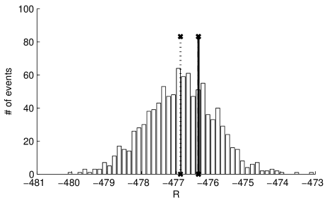
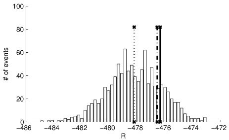
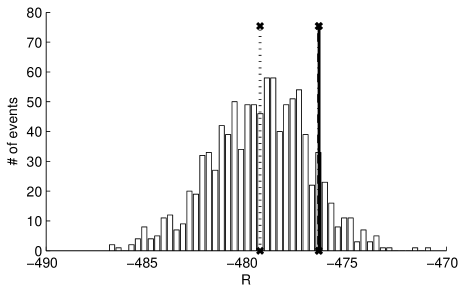
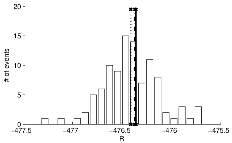
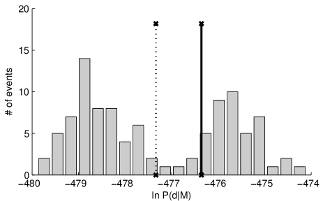
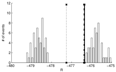
Figs.4, 5, and 6 highlight the influence of the protocol $\beta(t)$, all other parameters are the same. As can be seen the $R$-distributions produced are characterized by different mean values $\langle R\rangle$ and different widths $\sigma_{R}$. For $\beta^{\mathrm{poly}}(t)$ we get the narrowest and for $\beta^{\mathrm{lin}}(t)$ the widest distribution. Nevertheless the estimate $\ln\langle e^{R}\rangle$ barely changes and is for all three cases rather near to the exact value. Lower values of $\langle R\rangle$ and larger ones for $\sigma_{R}$ compensate each other (cf. (16)) leaving the estimate for the prior-predictive value almost the same. Still, as far as the error in the estimate is concerned, a narrow distribution of $R$ is advantageous and correspondingly $\beta^{\mathrm{poly}}(t)$ performs best.

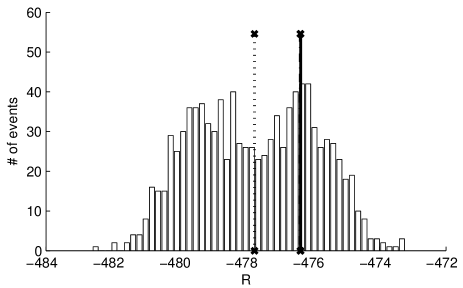
Making the trajectories longer, decreases the variance in $R$ further as can be seen in fig.7 but leaves less realizations $N_{c}$ for the exponential average $\langle e^{R}\rangle$. For the present case, however, the estimate for the prior-predictive value remains reliable.

Figure 7: Same as fig.4 using again the polynomial protocol (25) but now with $N_{c}=100$ runs consisting of $M=N=10^{7}$ steps each. The results are now $\langle R\rangle=-476.41$, $\sigma_{R}=0.3$, and $\ln\langle e^{R}\rangle=-476.370\pm 0.03$.

In the simulations we have observed that our method gives best results for many intermediate values of $\beta$. Therefore we have chosen for $M$ the maximal possible number, $M=N$, implying that $\beta$ is changed after each MC-step. From the discussion around eq.(14) this means that we are using our method in a regime where it is very similar to thermodynamic integration. This makes sense: for simple situations without equilibration problems thermodynamics integration works fine and our more general method yields comparable results for protocols which are near to a quasi-static process.

IV.2 Bimodal likelihood

The results obtained from thermodynamic integration for the bimodal case are displayed in figs. 8 and 9. It is clearly seen that the good performance of the unimodal case is not reached. The estimate for the prior-predictive value differs substantially from the exact value. This failure may be traced back to the incomplete equilibration between the two maxima of the likelihood. In the beginning of the simulation starting with the prior which is symmetric around $x=0$ the regions around $x=-1$ and $x=1$ are populated by the MC trajectories with roughly the same density. Later in the simulation transitions between the regions are extremely rare and consequently the different prefactors in (20) are not properly reproduced. It is this incomplete equilibration which is typical for multimodal distributions that impede a satisfactory performance of thermodynamic integration. As shown in fig.9 this failure cannot be mitigated by using longer trajectories since the equilibration over the barrier at $x=0$ is simply too slow.

Figure 8: Histogram of the logarithm of the prior-predictive value for the bimodal case as obtained from thermodynamic integration. Parameters and meaning of the lines are the same as in fig.(2). The result is now $\ln P_{\mathrm{td}}=-477.34\pm 0.07$ the exact value is still $\ln P=-476.358$

Figure 9: Same as fig.8 with parameters as in fig.3. The result is $\ln P_{\mathrm{td}}=-477.338\pm 0.16$.

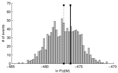
Results for the simulation of (12) for the bimodal case are displayed in figs.10 and 11. As can be seen the accuracy of the estimates for the prior-predictive value are much better than those from thermodynamic integration. In fact the quality of the results is comparable to those for the unimodal case. This may seem surprising since the bimodal structure of the histogram of $R$ clearly indicates that the realizations from the MC simulation are again captured by one of the two maxima of the likelihood. However, the weight factor $e^{R}$ differs for the two subsets of trajectories in exactly such a way as to produce the correct prefactors in front of the two parts of the posterior distribution, cf. (13). As a consequence a precise estimate of the prior-predictive value can be obtained although no final equilibration was reached. In this situation our method is hence superior to thermodynamic integration.

Figure 10: Histogram of $R$-values for the bimodal case as obtained by simulating (12) for the polynomial protocol (25) using $N_{c}=100$ runs consisting of $M=10^{6}$ $\beta$-steps and $N=10^{7}$ steps altogether. The results are $\langle R\rangle=-477.26$, $\sigma_{R}=0.15$, and $\ln\langle e^{R}\rangle=-476.38\pm 0.10$.

Figure 11: Same as fig.10 with $N_{c}=1000$ runs consisting of $M=10^{5}$ $\beta$-steps and $N=10^{6}$ steps all together resulting in $\langle R\rangle=-477.74$, $\sigma_{R}=0.06$, and $\ln\langle e^{R}\rangle=-476.371\pm 0.06$.

V Discussion

In the present note we have introduced a new method to numerically determine the prior-predictive value in a Bayesian inference problem from MC simulations. Our method derives from a variant of the Jarzynski equation Jar

$$\langle e^{-\beta W}\rangle=e^{-\beta\Delta F}$$ (27)

that allows to determine the free energy difference $\Delta F$ between two equilibrium states of a system at inverse temperature $\beta$ from an exponential average of the work $W$ done in a non-equilibrium transition between the two states. In statistical mechanics this equation has been used already to find differences in free energy from fast-growth simulations HeJa .

The method proposed in the present paper incorporates two approaches as limiting cases that are used already to determine the prior-predictive value, namely straight MC estimation and thermodynamic integration. The method was shown to work well in a simple unimodal example in which its efficiency was comparable with thermodynamic integration. It proved to be superior in the bimodal example. Our numerical implementation of both algorithms is not optimal. The amount of samples discarded in thermodynamic integration certainly can be reduced and the protocol $\beta^{\mathrm{poly}}$ for our procedure is not very sophisticated.

However, the example chosen with Gaussians for both prior and likelihood is rather remote from real applications so that a fine-tuning of the procedures for this special case seems to be somewhat ill-advised. A comparison of the methods when applied to a more realistic setup with the complications alluded to in the introduction and when implemented in a more optimal way is left for future work.

The main advantage of the new method presumably lies in its applicability to multimodal systems that resist naive equilibration approaches, and its great flexibility parametrized by a protocol function $\beta(t)$ which may be adapted to the particular problem under consideration. We therefore hope that the method will provide a useful extension of the box of tools available to perform model selection in the framework of Bayesian data analysis.

Acknowledgment: We are indebted to Prof. Dr. Volker Dose for many stimulating discussions.

References

- (1) Jaynes E. T., Probability Theory: The Logic of Science (Cambridge University Press, Cambridge, 2003)
- (2) Gelman A., Carlin J. B., Stern H. S., Rubin D. B., Bayesian Data Analysis (Chapman and Hall, London, 1995)
- (3) Leonhard T. and Hsu J. S. J., Bayesian Methods: An Analysis for Statisticians and Interdisciplinary Researchers (Cambridge University Press, Cambridge, 1999)
- (4) Bernardo J. M. et al. (eds.) Bayesian Statistics 7 (Oxford University Press, Oxford, 2003)
- (5) D’Agostini G., Rep. Prog. Phys. 66, 1383 (2003)
- (6) Dose V., Rep. Prog. Phys. 66, 1421 (2003)
- (7) R. Neal, Probabalistic Inference using Markov Chain Monte-Carlo Methods, Dept. of Computer Science, University of Toronto, 1993
- (8) von der Linden W., Preuss R., and Dose V., The prior-predictive value: A paradigm of nasty multi-dimensional integrals in Maximum Entropy and Bayesian Methods, von der Linden W. et al. (eds.) (Kluwer, Dordrecht, 1999)
- (9) Jarzynski C., Phys. Rev. Lett. 78, 2690 (1997)
- (10) Jarzynski C., J. Stat. Phys. 98, 77 (2000)
- (11) Crooks G., Phys. Rev. E61, 2361 (2000)
- (12) Seifert U., Phys. Rev. Lett. 95, 040602, (2005)
- (13) J. L. Lebowitz and H. Spohn, J. Stat. Phys. 95, 333 (1998)
- (14) Chatelain C., Temperature extended Jarzynski relation: Application to the numerical calculation of the surface tension”, cond-mat/0702044
- (15) Zwanzig R., J. Chem. Phys. 22, 1420 (1954)
- (16) Park S. and Schulten K., J. Chem. Phys. 120, 5946 (2004)
- (17) T. Speck and U. Seifert, Phys. Rev. E70, 066112 (2004)
- (18) Fox R. F., Proc. Natl. Acad. Sci. USA 100, 12537 (2003)
- (19) Gore J., Ritort F., and Bustamante C., Proc. Natl. Acad. Sci. USA 100, 12564 (2003)
- (20) Hummer G., J. Chem. Phys. 114, 7330 (2001)
- (21) Jarzynski, C., Phys. Rev. E73, 046105 (2006)
- (22) M. Daghofer, M. Konegger, H. G. Evertz, and W. von der Linden, Perfect Tempering arXiv:physics/0512167
- (23) D. A. Hendrix and C. Jarzynski, J. Chem. Phys. 114, 5974 (2001)