Quantum Bound on the Specific Entropy
in
Strong-Coupled Scalar Field Theory
M. Aparicio Alcalde , G. Menezes  and N. F. Svaiter  

Centro Brasileiro de Pesquisas Físicas-CBPF

Rua Dr. Xavier Sigaud 150, Rio de Janeiro, RJ, 22290-180, Brazil

Abstract

We discuss the $(g_{0}\,\varphi^{\,p})_{d}$ self-interacting scalar field theory, in the strong-coupling regime. We assume the presence of macroscopic boundaries confining the field in a hypercube of side $L$. We also consider that the system is in thermal equilibrium at temperature $\beta^{\,-1}$. For spatially bounded free fields, the Bekenstein bound states that the specific entropy satisfies the inequality $\frac{S}{E}<2\pi R$, where $R$ stands for the radius of the smallest sphere that circumscribes the system. Employing the strong-coupling perturbative expansion, we obtain the renormalized mean energy $E$ and entropy $S$ for the system up to the order $(g_{0})^{-\frac{2}{p}}$, presenting an analytical proof that the specific entropy also satisfies in some situations a quantum bound. Defining $\varepsilon_{d}^{(r)}$ as the renormalized zero-point energy for the free theory per unit length, the dimensionless quantity $\xi=\frac{\beta}{L}$ and $h_{1}(d)$ and $h_{2}(d)$ as positive analytic functions of $d$, for the case of high temperature, we get that the specific entropy satisfies $\frac{S}{E}<2\pi R\,\frac{h_{1}(d)}{h_{2}(d)}\,\xi$. When considering the low temperature behavior of the specific entropy, we have $\frac{S}{E}<2\pi R\,\frac{h_{1}(d)}{\varepsilon_{d}^{(r)}}\xi^{\,1-d}$. Therefore the sign of the renormalized zero-point energy can invalidate this quantum bound. If the renormalized zero point-energy is a positive quantity, at intermediate temperatures and in the low temperature limit, there is a quantum bound.
PACS numbers: 03.70+k, 04.62.+v

1 Introduction

There have been a lot of activities discussing classical and quantum fields in the presence of macroscopic boundaries. These subjects raise many interesting questions, since boundaries introduce a characteristic size in the theory. For example, in the field-theoretical description of critical phenomena, the confinement of critical fluctuations of an order parameter is able to generate long-range forces between the surfaces of a film. This is known as statistical mechanical Casimir effect [1] [2] [3] [4]. These long-range forces in statistical mechanical systems are characterized by the excess free energy due to the finite-size contributions to the free energy of the system. It should be noted that the statistical mechanical Casimir effect is still waiting for a satisfactory experimental verification. On the other hand, the electromagnetic Casimir effect [5], where neutral and perfectly conducting parallel plates in vacuum attract each other, has been tested experimentally with high accuracy. The introduction of a pair of conducting plates into the vacuum of the electromagnetic field alters the zero-point fluctuations of the field and thereby produces an attraction between the plates [6] [7] [8] [9]. A still open question is how the sign of the Casimir force depends on the topology, dimensionality of the spacetime, the shape of bounding geometry or others physical properties of the system [10] [11] [12] [13]. We should emphasize that the problem of the sign of the renormalized zero-point energy of free fields described by Gaussian functional integrals is crucial for the subject that we are interested to investigate in this paper.

Another basic question that has been discussed in this scenario, when quantum fields interact with boundaries, is about the issue that these systems may be subjected to certain fundamental bounds. One of these proposed bounds relates the entropy $S$ and the energy $E$ of the quantum system, respectively, with the size of the boundaries that confine the fields. This is known as the Bekenstein bound which is given by $S\leq 2\pi\,E\,R/\hbar\,c$, where $R$ stands for the radius of the smallest sphere that circumscribes the system [14] [15] [16] [17] [18]. Such bound was originally motivated by considerations of gravitational entropy, a consistency condition between black hole thermodynamics and ordinary statistical physics that could guarantee that the generalized second law of thermodynamics is respected, which states that the sum of the black-hole entropy and the entropy of the matter outside the black-hole does not decreases. For example, in a Schwarschild black-hole in a four-dimensional spacetime, the Bekenstein entropy, which is proportional to the area of the spherical symmetric system, exactly saturates the bound. When gravity is negligible, the bound must be valid for a variety of systems.

Although analytical proofs of this quantum bound on specific entropy for free fields has been proposed in the literature, many authors in the past criticized the bound [19] [20] [21] [22] [23]. Deutsch claims that the quantum bound is inapplicable as it stands to non-gravitating systems, since an absolute value of energy cannot be observed, and also that for sufficient low temperatures, a generic system in thermal equilibrium also violates the entropy bound. Unruh pointed out that for system with zero modes, the specific entropy cannot satisfy any bound. Many of these criticisms were answered by Bekenstein and collaborators. The problem of the low temperature systems was answered in Ref. [24] and the problem of systems with zero modes was answered in the Ref. [25]. An strong argument used in one of these examples is based in the fact that the renormalized zero-point energy of some free quantum field could be negative. Some authors claim that, if we take into account the boundaries responsible for the Casimir energy, it is possible to compensate their negative energy, yielding a positive total energy which respects the Bekenstein bound, although this is far from a simple problem [26].

In fact this last point that we pointed out, i.e., the objection raised against the violation of the Bekenstein bound for free fields, must be analyzed more carefully. The problem now confronting us is to prove that, although Casimir energy can be negative for some physical situation, the sum of the energy of the boundary and the Casimir energy will be positive. In other words, the contribution from the boundary would make the total energy of the system always positive for any configuration of the hyperplane when the Casimir energy is negative. How close the boundaries must be in such a way that the positive contribution from the rest mass of the boundary is always smaller than the modulus of the Casimir energy? Our conclusions from the above arguments is that, for example, in the case of the electromagnetic field, it is essential to construct a microscopic model where effects of dispersion and absorbtion must be taken into consideration. Many authors discussed the problem of quantization of the electromagnetic field in dispersive and absorptive linear dielectrics [27] [28] [29] [30]. The essential question that confronts us is the positivity of the total energy of any quantum system defined in a compact domain in any situation. The validity of the Bekenstein bound for configurations with negative Casimir energy depends on the answer for this last question. Our intention in this paper is not to study such deep and difficult question, introducing physically realistic boundary conditions, but only to discuss the situation of idealized mirror boundaries.

We may observe that another quite important situation has not been discussed systematically in the literature, at least as far we known. A step that remains to be derived is the validity of the bound for the case of interacting fields, which are described by non-Gaussian functional integrals, at least up to some order of the perturbation theory. Nonlinear interactions can change dramatically the energy spectrum of the system and this might lead to the overthrow of the bound [31] [32]. The difficulties that appear in the implementation of this program in the presence of macroscopic boundaries are well known. In systems where the translational invariance is lacking it is much harder to compute the Feynman diagrams then in the unbounded space. Nevertheless a regularization and renormalization procedure can in principle be carry out in any order of the perturbative expansion [33]. See for example refs. [34] [35] [36] [37], where the perturbative renormalization were presented in first and second order of the loop expansion in the $\lambda\varphi^{4}$ self-interacting scalar field theory. We would like to stress that the renormalization program is implement in a different way from unbounded or translational invariant systems because surface divergences appear.

The aim of this paper is to show for a given self-interaction field theory in which situations the specific entropy satisfies a quantum bound. For the answer of this important question, there are two different routes. The first one is to use the weak-coupling perturbative expansion. However, as we discussed, in the renormalization procedure appears surface divergences that forces one to introduce non-local counterterms. It is unclear for us how this affect the physical relevance of the results that can be obtained. There are some kind of problems for which the mean energy and the canonical entropy a system can easily be found for quantum fields defined in a simple connected bounded region. We can show that using the strong-coupling expansion one can evaluate the mean energy and the canonical entropy of the system in a regime in which quantum fluctuations dominate.

Therefore we study the $(g_{0}\,\varphi^{\,p})_{d}$ self-interacting scalar field theory in the strong-coupling regime. We assume the presence of macroscopic boundaries that confine the field in a hypercube of side $L$ and also that the system is in thermal equilibrium with a reservoir. We present an analytic proof that, up to the order $(g_{0})^{-\frac{2}{p}}$, the specific entropy satisfies in some situations a quantum bound. Defining $\varepsilon_{d}^{(r)}$ as the renormalized zero-point energy for the free theory per unit length, $\xi=\frac{\beta}{L}$ and $h_{1}(d)$ and $h_{2}(d)$ as positive analytic functions of $d$, for the case of high temperature, we get that the specific entropy satisfies the inequality $\frac{S}{E}<2\pi R\,\frac{h_{1}(d)}{h_{2}(d)}\,\xi$. When considering the low temperature behavior of the specific entropy, we have $\frac{S}{E}<2\pi R\,\frac{h_{1}(d)}{\varepsilon_{d}^{(r)}}\xi^{\,1-d}$. We are establishing a bound in the strong-coupled system in the following cases: in the high temperature limit and if the renormalized zero point-energy is a positive quantity, at intermediate temperatures and also in the low temperature limit.

In the weak-coupling perturbative expansion, the information about the boundaries can be implemented over the free two-point Schwinger function $G_{0}(m_{0};x-y)$ of the system. In the strong-coupling perturbative expansion, we have to deal with the problem of how the boundary conditions can be imposed. Let us briefly discuss the strong-coupling expansion in Euclidean field theory at zero temperature. The basic idea of the approach is the following: in a formal representation for the generating functional of complete Schwinger functions of the theory $Z(V,h)$, we treat the Gaussian part of the action as a perturbation with respect to the remaining terms of the functional integral, i.e., in the case for the $(g_{0}\,\varphi^{\,p})_{d}$ theory, the local self-interacting part, in the functional integral. In the generating functional of complete Schwinger functions, $V$ is the volume of the Euclidean space where the fields are defined and $h(x)$ is an external source. We are developing our perturbative expansion around the independent-value generating functional $Q_{0}(h)$ [38] [39] [40]. In the zero-order approximation, different points of the Euclidean space are decoupled since the gradient terms are dropped [41] [42] [43] [44].

The fundamental problem of the strong-coupling expansion is how to give meaning to the independent-value generating functional and to this representation for the Schwinger functional. One attempt is to replace the Euclidean space by a lattice made by hypercubes. A naive use of the continuum limit of the lattice regularization, where one simply makes use of the central limit theorem for the independent-value generating functional, leads to a Gaussian theory. A solution to this problem was presented by Klauder a long time ago [38] [40] [44]. The modification which allows us to avoid this limitation is a change in the usual definition of the measure in the functional integral, which possesses local translational invariance, by another one which is non-translational invariant.

Let us remark that, in the strong-coupling regime, assuming that the source is constant, we can perform the perturbative expansion around a independent-value generating function, up to the order $(g_{0})^{-\frac{2}{p}}$, and it is possible to split $\ln Z(V,h)$ in two contributions: one that contains only the independent-value generating function and other that contains the spectral zeta-function. Therefore, in order to obtain the thermodynamic quantities, one must proceed in two stages. First, one gives a operational meaning to the independent-value generating function; then, one consistently implements the boundary conditions in the strong-coupling regime. Since we are working in first order of perturbation theory, to implement boundary conditions, we use the spectral zeta-function method [45] [46]. For a complete review about the subject see for example refs. [47] [48]. Quite recently a very simple application of this formalism was presented [49], where it was considered an anharmonic oscillator in thermal equilibrium with a reservoir at temperature $\beta^{-1}$. Using the strong-coupling expansion, it was found the mean energy in the regime $\lambda\,\gg\,\omega$, up to the order $\frac{1}{\sqrt{\lambda}}$, where $\lambda$ and $\omega$ are the coupling constant and the frequency of the oscillator respectively.

The organization of the paper is as follows: In section II we discuss the strong-coupling expansion for the $(g_{0}\,\varphi^{\,p})_{d}$ theory. In section III we discuss he free energy and the spectral zeta-function of the system. In section IV we show that it is possible to obtain in some situations a quantum bound in the considered model. Finally, section V contains our conclusions. In the appendix A we present the Klauder’s result, as the formal definition of the independent-value generating functional derived for scalar fields in a $d$-dimensional Euclidean space. In the appendix B we prove that the spectral zeta-function $\zeta_{D}(s)$ evaluated in the extended complex plane at $s=0$ vanishes. To simplify the calculations we assume the units to be such that $\hbar=c=k_{B}=1$.

2 The strong-coupling perturbative expansion for scalar $(g_{0}\,\varphi^{\,p})_{d}$ theory

Let us consider a neutral scalar field with a $(g_{0}\,\varphi^{\,p})$ self-interaction, defined in a $d$-dimensional Minkowski spacetime. The vacuum persistence functional is the generating functional of all vacuum expectation value of time-ordered products of the theory. The Euclidean field theory can be obtained by analytic continuation to imaginary time allowed by the positive energy condition for the relativistic field theory. In the Euclidean field theory, we have the Euclidean counterpart for the vacuum persistence functional, that is, the generating functional of complete Schwinger functions. In a $d$-dimensional Euclidean space, the self-interaction contribution to the action is given by

$$S_{I}(\varphi)=\int d^{\,d}x\,\frac{g_{0}}{p\,!}\,\varphi^{\,p}(x).$$ (1)

The basic idea of the strong-coupling expansion at zero temperature is to treat the Gaussian part of the action as a perturbation with respect to the remaining terms of the action in the functional integral. Let us assume a compact Euclidean space with or without a boundary, where the volume of the Euclidean space is $V$. Let us suppose that there exists an elliptic, semi-positive, and self-adjoint differential operator $O$ acting on scalar functions on the Euclidean space. The usual example is $O=(-\Delta+m_{0}^{2}\,)$, where $\Delta$ is the $d$-dimensional Laplacian. The kernel $K(m_{0};\,x,y)\equiv\,K(m_{0};\,x-y)$ is defined by

$$K(m_{0};x-y)=\left(-\Delta+m_{0}^{2}\,\right)\delta^{d}(x-y).$$ (2)

Using the fact that the functional integral which defines $Z(V,h)$ is invariant with respect to the choice of the quadratic part, let us consider a modification of the strong-coupling expansion. We split the quadratic part in the functional integral which is proportional to the mass squared in two parts; one in the derivative terms of the action, and the other in the independent value generating functional. The Schwinger functional can be defined by a new formal expression for the functional integral given by

$$Z(V,h)=\exp\left(-\frac{1}{2}\int d^{d}x\,\int d^{d}y\frac{\delta}{\delta h(x)}K(m_{0},\sigma;x-y)\frac{\delta}{\delta h(y)}\right)\,Q_{0}(\sigma,h),$$ (3)

where $Q_{0}(\sigma,h)$, the new independent value functional integral, is given by

$$Q_{0}(\sigma,h)={\cal{N}}\int[d\varphi]\,\exp\Biggl{(}\int d^{d}x\,\biggl{(}-\frac{1}{2}\,\sigma\,m_{0}^{2}\,\varphi^{2}(x)-\,\frac{g_{0}}{p\,!}\,\varphi^{p}(x)+h(x)\varphi(x)\biggr{)}\Biggr{)},$$ (4)

and the modified kernel $K(m_{0},\sigma;x-y)$ that appears in Eq. (3), is defined by

$$K(m_{0},\sigma;x-y)=\left(-\Delta+(1-\sigma)m_{0}^{2}\,\right)\delta^{d}(x-y),$$ (5)

where $\sigma$ is a complex parameter defined in the region $0\leq\,\mbox{Re}\,\,(\sigma)<1$.

The factor ${\cal{N}}$ is a normalization that can be found using that $Q_{0}(\sigma,h)|_{\,h=0}=1$. Observe that the non-derivative terms which are non-Gaussian in the original action do appear in the functional integral that defines $Q_{0}(\sigma,h)$. At this point it is convenient to consider $h(x)$ to be complex. Consequently $h(x)=\mbox{Re}(h)+i\,\mbox{Im}(h)$. In the paper we are concerned with the case $\mbox{Re}(h)=0$.

Since we are assuming a spatially bounded system in equilibrium with a thermal reservoir at temperature $\beta^{-1}$, the strong-coupling expansion can be used to compute the partition function defined by $Z(\beta,\Omega,h)|_{\,h=0}$, where $h$ is a external source and we are defining the volume of the $(d-1)$ manifold as $V_{d-1}\equiv\,\Omega$. From the partition function we define the free energy of the system, given by $F(\beta,\Omega)=-\frac{1}{\beta}\ln\,Z(\beta,\Omega,h)|_{\,h=0}$. This quantity can be used to derive the mean energy $E(\beta,\Omega)$, defined as

$$E(\beta,\Omega)=-\frac{\partial}{\partial\beta}\ln Z(\beta,\Omega,h)|_{\,h=0},$$ (6)

and the canonical entropy $S(\beta,\Omega)$ of the system in equilibrium with a reservoir with a finite size given by

$$S(\beta,\Omega)=\biggl{(}1-\beta\frac{\partial}{\partial\beta}\biggr{)}\ln Z(\beta,\Omega,h)|_{h=0}.$$ (7)

In the next section we will show that in a particular situation it is possible, up to the order $(g_{0})^{-\frac{2}{p}}$ to split $\ln Z(\beta,\Omega,h)$ in two parts: the first one that contains only the independent-value generating function and the second one that has the information on the boundary condition and it is given by derivative of the spectral zeta-function defined in the extended complex plane in $s=0$ .

3 The independent-value generating function and the spectral zeta-function

We are interested in global quantities. For simplicity we are assuming that the external source $h(x)$ is constant. In this situation we call $Z(V,h)$ as a generating function. Since we are introducing boundaries in the domain where the field is defined, the spectrum of the operator $D=\left(-\Delta+(1-\sigma)m_{0}^{2}\,\right)$ has a denumerable contribution, and an analytic regularization procedure can be used to control the divergences of the theory. In order to impose boundary conditions the functional integral must be taken over functions restricted to the geometric configurations. At zero temperature, in the leading-order approximation (up to the to the order $(g_{0})^{-\frac{2}{p}}$) we can write the logarithm of the generating function as

$$\ln Z(\beta,\Omega,h)=\frac{1}{Q_{0}(\sigma,h)}\frac{\partial^{2}}{\partial\,h^{2}}\,Q_{0}(\sigma,h)\left(-\frac{\alpha}{2}+\frac{1}{2}\frac{d}{ds}\,\zeta_{D}(s)|_{\,s=0}\right),$$ (8)

where $\alpha$ is a infinite constant and $\zeta_{D}(s)$ is the spectral zeta-function associated with the elliptic operator $D$.

Let us consider now the situation in which the system is finite along each one of the spatial dimensions, i.e., $x_{i}\in\,\,[0,L]$, $i=1,2,...,d-1$. For the Euclidean time we assume periodic boundary conditions (Kubo-Martin-Schwinger KMS [50] [51] conditions) and for the Euclidean spatial dimensions we assume Dirichlet boundary conditions. We call this latter situation ”hard” boundaries. See for example the Ref. [52]. For different kinds of confining boundaries see [53] [54]. The choice of the hard boundary provides an easy solution to the eigenvalue problem, so that explicit and complete calculation using the spectral-zeta function can be performed without difficulty.

It follows that the operator $D$ has the spectrum given by $\lambda_{\,n_{1},\,...\,,\,n_{d}}\,$ where

$$\lambda_{\,n_{1},\,...\,,\,n_{d}}\,=\,\biggl{[}\biggl{(}\frac{n_{1}\pi}{L}\biggr{)}^{2}+...+\biggl{(}\frac{n_{d-1}\pi}{L}\biggr{)}^{2}+\biggl{(}\frac{2n_{d}\,\pi}{\beta}\biggr{)}^{2}+(1-\sigma)m_{0}^{2}\,\biggr{]},$$ (9)

$n_{1},n_{2},...\,,n_{d-1}$ are natural numbers different from zero, since we are choosing Dirichlet boundary conditions and $n_{d}$ are integer numbers. The spectral zeta-function associated with the operator $D$ in this situation reads

$$\zeta_{D}(s)=\,\sum_{n_{1},...,\,n_{d}}^{\infty\,\,\,\,\,_{{}^{\prime}}}\lambda_{\,n_{1},...,\,n_{d}}^{-s}\,,$$ (10)

where $s$ is a complex parameter, and the prime sign means that the term $n_{1}=0,n_{2}=0,..,n_{d-1}=0$ must be excluded. The series above converges for Re$\,s>\,\frac{d}{2}$ and its analytic continuation defines a meromorphic function of $s$, analytic at $s=0$. Since we should have to introduce an arbitrary parameter $\mu$ with dimension of a mass to implement the analytic procedure with dimensionless quantities, we have scaling properties.

Using $n$ as a general index instead of $n_{1},...,\,n_{d}$, the scaling properties follows from the fact that

$$\zeta_{\,\mu D}(s)=\sum_{n}^{\infty}(\,\mu^{-2}\,\lambda_{\,n})^{-s}=\mu^{2s}\sum_{n}^{\infty}\lambda_{\,n}^{-s}=\mu^{2s}\zeta_{D}(s)\,.$$ (11)

Therefore we have

$$\frac{1}{2}\frac{d}{ds}\,\zeta_{\,\mu D}(s)|_{\,s=0}=\frac{1}{2}\frac{d}{ds}\,\zeta_{D}(s)|_{\,s=0}+\frac{1}{2}\ln\mu^{2}\,\zeta_{D}(s)|_{\,s=0}.$$ (12)

Before continuing, we would like to discuss two points. The first one is the fact that for different boundary condition, as, for example, Neumann boundary conditions in all the hyperplanes or periodic boundary conditions in all the spatial directions, the presence of the zero-mode can make the calculations more involved. Studying a two-dimensional spacetime $T\times S^{1}$ and also $T\times S^{3}$, Dowker [55] discussed how the spatial zero mode contributes to the free energy. The zero-mode problem was also discussed by Dowker and Kirsten [56]. Elizalde and Tort [57] discussed the contribution to the thermal energy coming from the spatial zero mode in a system defined in a manifold with non-trivial topology; being more specific these authors studied a massive scalar field in $S^{1}\times S^{3}$ geometry. Kirsten and Elizalde discussed the Casimir energy of a massive scalar field in a general $(2+1)$ - dimensional toroidal spacetime. For the massless case they excluded the $n_{1}=n_{2}=0$ mode [58]. They discussed also in an ultrastatic $d$-dimensional spacetime how the ambiguity of the Casimir energy is related to the $B_{\frac{d}{2}}$. The entropy bound related to various fields in the $R\times\,S^{3}$ geometry was also discussed by many authors. See for example the Refs. [59] [60]. It is important to remark that this zero mode problem does not appear in the calculations that we are presenting, since we are choosing Dirichlet boundary conditions in all hyperplanes, excluding the possibility of the spatial zero mode. The generalized Bekenstein bound for systems with the spatial zero mode must be taken in consideration to extend the results of the paper.

The second point is that it is possible to show that there is no scaling in the situation that we are interested in. The spectral zeta-function is related to the heat-kernel or diffusion operator via a Mellin transform. The trace of the diffusion operator is the integral of the diagonal part of the heat-kernel over the manifold. It is possible to perform an asymptotic expansion for the heat-kernel and this asymptotic expansion shows that the spectral zeta-function is a meromorphic function of the complex variable $s$ possessing simple poles where the residues of the poles depends on the $B_{n}$ coefficients which depends on the Seeley-DeWitt coefficients, the second fundamental form on the boundary and the induced geometry on the boundary. See for example the Ref. [61] [62]. It is possible to show that the polar structure of the analytic extension of the spectral zeta function in a compact manifold with boundary is given by

$$\zeta_{D}(s)=\frac{1}{(4\pi)^{\frac{d}{2}}}\frac{1}{\Gamma(s)}\Bigg{[}\sum_{n=0}^{\infty}\frac{B_{n}}{n-\frac{d}{2}+s}+g_{2}(s)\Biggr{]},$$ (13)

for $n$ integer or odd-half integer, where $g_{2}(s)$ is an analytic function in ${\bf C}$. As was stressed by Blau et al [63], in a four dimensional flat spacetime with massless particles and thin boundaries the geometric coefficient $B_{2}$ vanishes. The spectral zeta function has poles at $s=1$, $s=2$, and so on. There would be a pole at $s=0$, but is cancelled out by the pole in the gamma function. Therefore $\zeta_{D}(s)|_{s=0}=B_{\frac{d}{2}}$. For the case of hypercube with Dirichlet boundary conditions we prove in the appendix B that the spectral zeta-function in $s=0$ is zero, consequently $B_{\frac{d}{2}}=0$ and there is no scaling in the theory. We shall come back to this point in the conclusions.

Let us study in Eq. (8) the contribution arising from the spectral zeta-function which takes into account the geometric constraints upon the scalar field. Using the spectrum of the $D$ operator given by Eq. (9) and the definition of the spectral zeta-function given by Eq. (10), we get that the derivative of the spectral zeta-function in $s=0$ yields

$$\frac{d}{ds}\,\zeta_{D}(s)|_{\,s=0}=-\,\sum_{\vec{n}_{d-1}=1}^{\infty}\sum_{n_{d}=-\infty}^{\infty}\Biggl{(}\ln\biggl{(}\biggl{(}\frac{\pi\,\beta\,q}{L}\biggr{)}^{2}+(2\pi n_{d})^{2}\biggr{)}+\ln\Biggl{(}1+\frac{a^{2}\beta^{2}}{4n_{d}^{2}L^{2}+q^{2}\beta^{2}}\Biggr{)}\Biggr{)},$$ (14)

where $\vec{n}_{d-1}=(n_{1},n_{2},...,n_{d-1})$, $q^{2}=n_{1}^{2}+n_{2}^{2}+...+n_{d-1}^{2}$ and $a^{2}=\biggl{(}\frac{(1-\sigma)m_{0}^{2}L^{2}}{\pi^{2}}\biggr{)}$. Note that in Eq. (14) we are using that $\zeta_{D}(s)|_{\,s=0}=0$. Using the following identity [64]

$$\ln\Biggl{(}\biggl{(}\frac{\pi\,\beta\,q}{L}\biggr{)}^{2}+(2\pi n_{d})^{2}\Biggr{)}=\int_{1}^{(\frac{\pi\,\beta\,q}{L})^{2}}\,\frac{d\theta^{2}}{\theta^{2}+(2\pi n_{d})^{2}}+\ln\Bigl{(}1+(2\pi n_{d})^{2}\Bigr{)}\,,$$ (15)

we can see that the first term in the right hand side of Eq. (14) gives a divergent contribution. To proceed we use another useful identity given by

$$\sum_{n_{d}=-\infty}^{\infty}\,\frac{1}{\theta^{2}+(2\pi n_{d})^{2}}=\frac{1}{2\theta}\biggl{(}1+\frac{2}{e^{\theta}-1}\biggr{)}.$$ (16)

Using both identities given by Eq. (15) and Eq. (16), it is possible to express the double summation that appears in Eq. (14) by a single summation given by

$$\sum_{\vec{n}_{d-1}=1}^{\infty}\sum_{n_{d}=-\infty}^{\infty}\ln\Biggl{(}\biggl{(}\frac{\pi\,\beta\,q}{L}\biggr{)}^{2}+(2\pi n_{d})^{2}\Biggr{)}=2\sum_{\vec{n}_{d-1}=1}^{\infty}\int_{1}^{\bigl{(}\frac{\pi\,\beta\,q}{L}\bigr{)}}\,d\theta\biggl{(}\frac{1}{2}+\frac{1}{e^{\theta}-1}\biggr{)}+\alpha_{1},$$ (17)

where $\alpha_{1}=\sum_{\vec{n}_{d-1}=1}^{\infty}\sum_{n_{d}=-\infty}^{\infty}\ln\Bigl{(}1+(2\pi n_{d})^{2}\Bigr{)}$. Carrying out the $\theta$ integration, we finally arrive that Eq. (17) can be written as

$$\sum_{\vec{n}_{d-1}=1}^{\infty}\sum_{n_{d}=-\infty}^{\infty}\ln\Biggl{(}\biggl{(}\frac{\pi\,\beta\,q}{L}\biggr{)}^{2}+(2\pi n_{d})^{2}\Biggr{)}=2\sum_{\vec{n}_{d-1}=1}^{\infty}\Biggl{(}\frac{\pi\,\beta\,q}{2L}+\ln\biggl{(}1-e^{-\frac{\pi\,\beta\,q}{L}}\biggr{)}\Biggr{)}+\alpha_{2}\,,$$ (18)

where $\alpha_{2}=\alpha_{1}-\sum_{\vec{n}_{d-1}=1}^{\infty}\Bigl{(}1+2\ln(1-e^{-1})\Bigr{)}$. Since this divergent contribution $\alpha_{2}$ is $\beta$-independent we will see that it can be eliminated using the third law of thermodynamics. The first term on the right side of Eq. (18) is a divergent contribution, corresponding to the zero-point energy term. Using the following mathematical result [65] [66] given by

$$\prod_{n=-\infty}^{\infty}\Biggl{(}1+\frac{a^{2}}{n^{2}+b^{2}}\Biggr{)}=\frac{\sinh^{2}(\pi\sqrt{a^{2}+b^{2}})}{\sinh^{2}(\pi\,b)}\,,$$ (19)

we can write the last term of Eq. (14) in a more manageable way. Using the Eq. (18) and Eq. (19), the derivative of the spectral zeta-function in $s=0$ can be rewritten as

$$\frac{d}{ds}\,\zeta_{D}(s)|_{\,s=0}=-2\sum_{\vec{n}_{d-1}=1}^{\infty}\left[\ln\left(\frac{\sinh\Bigl{(}\frac{\pi\beta}{2L}\sqrt{q^{2}+a^{2}}\,\Bigr{)}}{\sinh\Bigl{(}\frac{\pi\beta q}{2L}\Bigr{)}}\right)+\ln\biggl{(}1-e^{-\frac{\pi\,\beta\,q}{L}}\biggr{)}+\frac{\pi\,\beta\,q}{2L}\right]-\alpha_{2}\,.$$ (20)

It is possible to show (see appendix A) that, in the finite temperature case, the independent-value generating function $Q_{0}(\sigma,h)$ satisfies $Q_{0}(\sigma,h)|_{{}_{h=\sigma=0}}=1$, and

$$\frac{\partial^{2}}{\partial\,h^{2}}\,Q_{0}(\sigma,h)|_{\,h=\sigma=0}=\frac{\Gamma(\frac{2}{p})}{2p\,g_{0}^{\frac{2}{p}}(p\,!)^{\frac{p}{2}}}.$$ (21)

In the next section we show that it is possible to obtain a quantum bound in the spatially bounded system defined by a self-interacting scalar field in the strong-coupling regime in high temperatures. As we will see, for the cases of intermediate or low temperatures, the sign of the renormalized zero-point energy is crucial for the validity of a quantum bound for the specific entropy.

4 The specific entropy for strongly coupled $(g_{0}\,\varphi^{\,p})_{d}$ theory

In this section we compute the specific entropy $\frac{S}{E}$ of the system. For simplicity, let us define $\ln Z(\beta,\Omega,h)|_{\,h=0}=\ln Z(\beta,\Omega)$. From Eq. (6) and Eq. (7), and using for simplicity that the mean energy $E(\beta,\Omega)=E$ and the entropy $S(\beta,\Omega)=S$, the specific entropy is given by

$$\frac{S}{E}=\beta-{\ln Z(\beta,\Omega)}\biggl{(}\frac{d}{d\beta}\ln Z(\beta,\Omega)\biggr{)}^{-1}\,.$$ (22)

Substituting Eq. (20) and Eq. (21) in Eq. (8) we have that $\ln Z(\beta,\Omega)$ is given by

$$\ln Z(\beta,\Omega)=-\frac{\Gamma(\frac{2}{p})}{2p\,(p\,!)^{\frac{p}{2}}g_{0}^{\frac{2}{p}}}\left(\frac{\alpha\,^{\prime}}{2}+I_{2}(\beta)\right)\,,$$ (23)

where $\alpha\,^{\prime}=\alpha+\alpha_{2}$ and the quantity $I_{2}(\beta)$ is given by

$$I_{2}(\beta)=\sum_{\vec{n}_{d-1}=1}^{\infty}\left[\ln\left(\frac{\sinh\Bigl{(}\frac{\pi\beta}{2L}\sqrt{q^{2}+a^{2}}\,\Bigr{)}}{\sinh\Bigl{(}\frac{\pi\beta q}{2L}\Bigr{)}}\right)+\ln\biggl{(}1-e^{-\frac{\pi\,\beta\,q}{L}}\biggr{)}+\frac{\pi\,\beta\,q}{2L}\right]\,.$$ (24)

Defining $C_{1}$ and $C_{2}=\,-\frac{2C_{1}}{\alpha\,^{\prime}}$ that depend only of $p$ and $g_{0}$ and do not depend on $\beta$ as

$$C_{1}=-\frac{\alpha\,^{\prime}\,\Gamma(\frac{2}{p})}{4p\,(p\,!)^{\frac{p}{2}}g_{0}^{\frac{2}{p}}}\,,$$ (25)

the quantity $\ln Z(\beta,\Omega)$ can be written in a general form as

$$\ln Z(\beta,\Omega)=C_{1}-C_{2}\,I_{2}(\beta).$$ (26)

It is worth to mention that the quantity $C_{1}$ corresponds to a divergent expression, $C_{2}$ is finite and the summation term in the right-hand side of Eq. (20) is proportional to the zero-point energy. In order to renormalize $\ln Z(\beta,\Omega)$ we first can use the third law of thermodynamics. The derivative of $\ln Z(\beta,\Omega)$ with respect of $\beta$ yields

$$\frac{d}{d\beta}\ln Z(\beta,\Omega)=-C_{2}\,\frac{d}{d\beta}I_{2}(\beta),$$ (27)

where the derivative of $I_{2}(\beta)$ with respect to $\beta$ is given by

$$\frac{d}{d\beta}I_{2}(\beta)=\frac{\pi}{2L}\sum_{\vec{n}_{d-1}=1}^{\infty}\left(\Biggl{(}\sqrt{q^{2}+a^{2}}\,\coth\biggl{(}\frac{\pi\beta}{2L}\sqrt{q^{2}+a^{2}}\,\biggr{)}-q\,\coth\biggl{(}\frac{\pi\beta\,q}{2L}\biggr{)}\Biggr{)}+\frac{2\,q}{e^{\frac{\pi\,\beta\,q}{L}}-1}+q\right)\,.$$ (28)

Using the definition of the mean energy given by Eq. (6), Eq. (27) and Eq. (28) we have that the unrenormalized mean energy is given by

$$E=\frac{\pi\,C_{2}}{2L}\sum_{\vec{n}_{d-1}=1}^{\infty}\left(\Biggl{(}\sqrt{q^{2}+a^{2}}\coth\biggl{(}\frac{\pi\beta}{2L}\sqrt{q^{2}+a^{2}}\,\biggr{)}-q\,\coth\biggl{(}\frac{\pi\beta\,q}{2L}\biggr{)}\Biggr{)}+\frac{2\,q}{e^{\frac{\pi\,\beta\,q}{L}}-1}+q\right)\,.$$ (29)

For the case $a=0$, i.e., the massless case, using the Eq. (25) we get that the unrenormalized mean energy $E(\beta,\Omega)$ becomes

$$E(\beta,\Omega)|_{a=0}=\frac{\pi\,\Gamma(\frac{2}{p})}{4p\,(p\,!)^{\frac{p}{2}}\,g_{0}^{\frac{2}{p}}L}\,\sum_{\vec{n}_{d-1}=1}^{\infty}\left(\frac{2\,q}{e^{\frac{\pi\,\beta\,q}{L}}-1}+q\right)\,.$$ (30)

The formula above has the simple interpretation of being phase space sums over the mean energy of each mode, where the zero-point energy is included. Note that the divergence that appear in the mean energy given by the Eq. (30) is coming from the zero-point energy, which is given by

$$E_{0}=\frac{\pi}{2L}\sum_{\vec{n}_{d-1}=1}^{\infty}(n_{1}^{2}+n_{2}^{2}+...+n_{d-1}^{2})^{\frac{1}{\,2}}\,,$$ (31)

and its sign is given by the ratio between the first and the second terms of the right-hand side of Eq. (30), for a negative zero-point energy. The sign of the renormalized mean energy will be discussed in details later in this section.

Let us briefly discuss how to find the renormalized zero-point energy. An analytic regularization gives the renormalized zero-point energy. Using the definition of the Epstein-zeta function given by

$$A(a_{1},a_{2},...,a_{k};2s)=\sum_{\vec{n}_{k}=-\infty}^{\infty}(a_{1}n_{1}^{2}+a_{2}n_{2}^{2}+...+a_{k}n_{k}^{2})^{-s}\,,$$ (32)

we can find the analytic extension of the Epstein-zeta function in the complex plane, in particular at $s=-\frac{1}{2}$, to define the Casimir energy. The structure of the divergences of the analytic extension of the Epstein-zeta function is well known in the literature [10] [67] [68] [69]. The renormalized zero-point energy $E_{0}^{\,r}$ is defined as the finite part of a meromorphic function that possesses simple poles. Details of this calculations can be found in refs. [11] [70]. As stressed in the Ref. [63] there is an ambiguity in the renormalization procedure to find the Casimir energy.

It is possible to prove that, in a regularization of an ill defined quantity, if the introduction of a exponential cut-off yields a analytical function with a pole in the origin, the analytic extension of the generalized zeta-function, or the zeta-function method, is equivalent to the application of a cut-off with the subtraction of the singular part at the origin [71] [72]. Once we accept the advantage of the zeta-function method over the cut-off method with the subtraction of the polar terms, due to the fact that it is an analytical extension method, we face a problem: the non-trivial scaling behavior of the vacuum energy. This follows from the fact that in an analytic extension method it is necessary to introduce a mass parameter $\mu$, i.e., a normalization scale to keep the Epstein-zeta function dimensionless for all values of $s$. If we consider a change in the normalization scale $\mu\rightarrow\,\mu^{\prime}$, it is possible to show that in a $d$-dimensional spacetime, the ambiguity of the renormalized zero-point energy is related to the $B_{\frac{d}{2}}$ coefficient by the expression:

$$E_{0}^{\,r}(\mu^{\prime})=E_{0}^{\,r}(\mu)-\mu\,\frac{B_{\frac{d}{2}}}{(4\pi)^{d/2}}\,\ln\Biggl{(}\frac{\mu^{\prime}}{\mu}\Biggr{)}.$$ (33)

Although, in general situations, there is an ambiguity in the renormalization procedure, in our case $\zeta_{D}(s)|_{\,s=0}=B_{\frac{d}{2}}=0$. Therefore there is no scaling in the theory and consequently the renormalized zero-point energy does not depend on the renormalized scale $\mu$.

Note that although in the expression for the renormalized mean energy, up to the order $(g_{0})^{-\frac{2}{p}}$, the coupling constant appears, we are interested only in the ratio $\frac{S}{E}$, and the dependence of the coupling constant disappears. It is important to stress that this happens only because in the strong-coupling expansion, up to the order $(g_{0})^{-\frac{2}{p}}$, we are able to split $\ln Z$ into two contributions: the first one proportional to the spectral-zeta function and the second one that has a contribution from the independent-value generating function $Q_{0}(\sigma,h)$.

After this discussions we are able to present the entropy of the system. Substituting Eq. (26) and Eq. (27) in the definition of the entropy given by Eq. (7), we have that the entropy of the system can be written as

$$S=C_{1}-\beta C_{2}\left(\frac{I_{2}(\beta)}{\beta}-\frac{d}{d\beta}I_{2}(\beta)\right)\,.$$ (34)

A system with a unique ground state corresponds to a state of vanishing entropy at zero temperature. For systems with degenerate ground states this property is also valid if the entropy is a extensive quantity. Since at zero temperature the system goes to a non-degenerate ground state, the entropy must go to zero. The expression of the entropy given by Eq. (34) must satisfy the third law of thermodynamics, i.e., the entropy of a system has a limiting property that $\lim_{\beta\rightarrow\infty}S=0$. To proceed, lets analyze the limit given by

$$\lim_{\beta\rightarrow\infty}\frac{I_{2}(\beta)}{\beta}=\lim_{\beta\rightarrow\infty}\frac{d}{d\beta}I_{2}(\beta)=\frac{\pi a^{2}}{2L}\sum_{\vec{n}_{d-1}=1}^{\infty}\frac{1}{\sqrt{q^{2}+a^{2}}\,+q}+\frac{\pi}{2L}\sum_{\vec{n}_{d-1}=1}^{\infty}q\,.$$ (35)

Substituting Eq. (35) in Eq. (34), and using the third law of thermodynamics, we get

$$\lim_{\beta\rightarrow\infty}S=C_{1}=\,0\,.$$ (36)

Therefore the first step to find a finite result for $\ln Z(\beta,\Omega)$ was achieved, since we were able to renormalize $C_{1}$ to zero using the third law of thermodynamics. After this step we have

$$\ln Z(\beta,\Omega)=-C_{2}\,I_{2}(\beta)\,.$$ (37)

Substituting Eq. (37) in Eq. (22) we can see that for the case $a=0$, i.e., the massless case, the quotient $\frac{S}{E}$ yields

$$\frac{S}{E}=2\pi R\,T_{d}(\xi)\,,$$ (38)

where we are defining the dimensionless variable $\xi$ given by $\xi=\beta/L$. Since the field is confined in a hypercube, the radius of the smallest $(d-1)$-dimensional sphere that circumscribes this system should be given by $R=\frac{1}{2}\sqrt{(d-1)}\,L$. The function $T_{d}(\xi)$ defined in Eq. (38) is given by

$$T_{d}(\xi)=\frac{1}{\pi\sqrt{d-1}}\,\frac{\xi\,P_{d}(\xi)+R_{d}(\xi)}{\varepsilon_{d}^{(r)}+P_{d}(\xi)}\,,$$ (39)

where $\varepsilon_{d}^{(r)}=LE_{0}^{(r)}$ and the positive functions $P_{d}(\xi)$ and $R_{d}(\xi)$ are defined respectively by

$$P_{d}(\xi)=\sum_{\vec{n}_{d-1}=1}^{\infty}\pi\,q\left(e^{\pi\,\xi\,q}-1\right)^{-1}$$ (40)

and

$$R_{d}(\xi)=-\sum_{\vec{n}_{d-1}=1}^{\infty}\ln\left(1-e^{-\pi\,\xi\,q}\right)\,.$$ (41)

Now let us study the function $T_{d}(\xi)$ given by Eq. (38). The quantum bound holds whenever $T_{d}(\xi)\leq 1$ for all values of $\xi$. From the definition of the function $T_{d}(\xi)$, given by Eq. (39), we have that $T_{d}(\xi)$ has a divergent value only if the renormalized zero-point energy is negative. For the point $\xi=\xi_{0}$ which satisfies $\varepsilon_{d}^{(r)}+P_{d}(\xi_{0})=0$, the quantum bound is invalidated.

Numerical calculations can help us understand the quantum bound. In the Fig. (1) we present the plot of the function $T_{d}(\xi)$ in the case of $d=3$ over the interval $0<\xi<2$. Since the renormalized zero-point energy is positive [70], the function $T_{d}(\xi)$ is also positive for all values of $\xi$. There is a maximum for some value of $\xi$ that we are calling $\xi_{max}$, which is near one. For this case there is a quantum bound. In Fig.(2) we present the function $T_{d}(\xi)$ in the case of $d=4$ over the interval $0<\xi<2$. Since in this case the renormalized zero-point energy is negative, we have that for some value of $\xi=\xi_{0}$, the function $T_{d}(\xi)$ diverges. There exists a critical value $\xi_{c}$ where, for $\xi\,>\,\xi_{c}$, the specific entropy is unbounded above.

Let us analyze two cases. The first one is when the renormalized zero-point energy is positive (see Fig. 1) and a maximum value for $T_{d}(\xi)$ appears. The second case, with a negative renormalized zero-point energy, invalidate the quantum bound. For even dimensional spacetime, the renormalized zero-point energy is always negative. For the odd dimensional case, it is known that for $d\leq 29$ this quantity is positive and for $d>29$ it changes the sign [11].

For the cases of positive renormalized zero-point energy, an equation for the maximum value of $T_{d}(\xi)$ can be found. The equation for the maximum is given by $R_{d}(\xi_{max})=\varepsilon_{d}^{(r)}\,\xi_{max}$. Substituting this $\xi_{max}$ in Eq. (39) we can find that $T_{d}(\xi_{max})=\frac{\xi_{max}}{\pi\sqrt{d-1}}$. Using the same procedure in Eq. (38) we get $\frac{S}{E}=\beta_{max}$, where $\beta_{max}=L\,\xi_{max}$. Therefore we can conclude that for odd space-time dimensions $d\leq 29$ there exists a maximum value for the function $T_{d}(\xi)$.

We can see that the maximum value of $T_{d}(\xi)$ depends on the renormalized zero-point energy, where for the case $d=3$ is less than one. To prove that, for odd $d\leq\,29$, we have that $T_{d}(\xi)$ satisfies the inequality $T_{d}(\xi)<1$, let us define an auxiliary function $R\,^{\prime}_{d}(\xi)$ that satisfies $R_{d}(\xi)<R\,^{\prime}_{d}(\xi)$. This function is given by

$$R\,^{\prime}_{d}(\xi)=-\int_{\Omega_{R}}d\Omega_{d-1}\int_{0}^{\infty}\,dr\,r^{d-2}\ln\left(1-e^{-\pi\,\xi\,r}\right)\,,$$ (42)

where the angular domain of integration $\Omega_{R}$ correspond to the region where $r_{i}>0$. Performing this integral [66] we have that

$$R\,^{\prime}_{d}(\xi)=S_{d-1}\,\Gamma(d-1)\,\zeta(d)\biggl{(}\frac{1}{\pi\xi}\biggr{)}^{d-1}\,.$$ (43)

where the angular term is $S_{d-1}=\frac{(\sqrt{\pi})^{d-1}}{2^{d-2}\Gamma(\frac{d-1}{2})}$. Using the Eq. (43) in the equation for the maximum, i.e., $R_{d}(\xi_{max})=\varepsilon_{d}^{(r)}\,\xi_{max}$, we can find that $\xi_{max}<\xi^{\prime}_{max}$, where

$$\xi^{\prime}_{max}=\left(\frac{2}{(2\sqrt{\pi})^{d-1}}\frac{\Gamma(d-1)\,\zeta(d)}{\Gamma(\frac{d-1}{2})\,\varepsilon_{d}^{(r)}}\right)^{\frac{1}{d}}\,,$$ (44)

and we have that $T_{d}(\xi_{max})<\frac{\xi^{\prime}_{max}}{\pi\sqrt{d-1}}$. In the table 1 we present the maximum values for $d=3$ until $d=29$ for odd $d$’s.

d	3	5	7	9	11	13
$\varepsilon_{d}^{(r)}$	$4.1\times 10^{-2}$	$6.2\times 10^{-3}$	$1.1\times 10^{-3}$	$2.2\times 10^{-4}$	$4.4\times 10^{-5}$	$9.4\times 10^{-6}$
$T_{d}(\xi_{max})<$	0.3763	0.2645	0.2303	0.2130	0.2025	0.1953

d	15	17	19	21	23	25
$\varepsilon_{d}^{(r)}$	$2.0\times 10^{-6}$	$4.5\times 10^{-7}$	$1.0\times 10^{-8}$	$2.2\times 10^{-8}$	$5.0\times 10^{-9}$	$1.1\times 10^{-9}$
$T_{d}(\xi_{max})<$	0.1901	0.1861	0.1829	0.1804	0.1784	0.1769

d	27	29	31
$\varepsilon_{d}^{(r)}$	$2.3\times 10^{-10}$	$3.0\times 10^{-11}$	$-1.1\times 10^{-11}$
$T_{d}(\xi_{max})<$	0.1761	0.1781	no maximum

Figure 1: $T_{d}(\xi)$ as a function of $\xi$ for the case of positive renormalized zero-point energy for $d=3$.

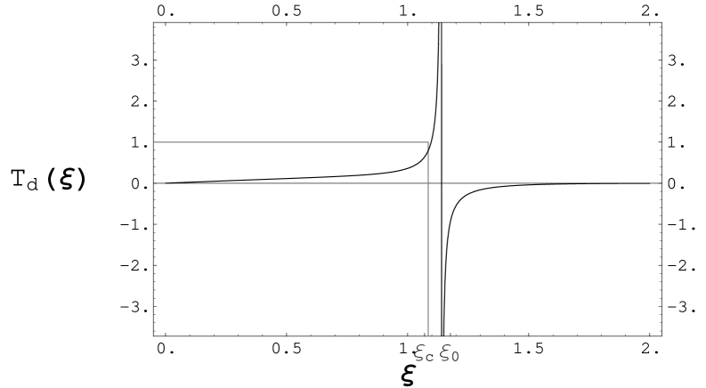
Figure 2: $T_{d}(\xi)$ as a function of $\xi$ for the case of negative renormalized zero-point energy for $d=4$.

Until now we studied the quantum bound for general dimensions based on the summations given by Eq. (40) and Eq. (41). Nevertheless we can find an upper bound function $T\,^{\prime}_{d}(\xi)$ of the function $T_{d}(\xi)$ which is more manageable. For this purpose, in a similar way as we have defined the function $R\,^{\prime}_{d}(\xi)$, let us define also the auxiliary functions $P\,^{\prime}_{d}(\xi)$ and $P\,^{\prime\prime}_{d}(\xi)$, that satisfy

$$P_{d}(\xi)<P\,^{\prime}_{d}(\xi)\,,$$ (45)

and

$$P_{d}(\xi)>P\,^{\prime\prime}_{d}(\xi)\,,$$ (46)

so that the specific entropy satisfies the following inequality

$$\frac{S}{E}<2\pi R\,T\,^{\prime}_{d}(\xi)\,,$$ (47)

where

$$T\,^{\prime}_{d}(\xi)=\frac{1}{\pi\sqrt{d-1}}\,\frac{\xi\,P\,^{\prime}_{d}(\xi)+R\,^{\prime}_{d}(\xi)}{\varepsilon_{d}^{(r)}+P\,^{\prime\prime}_{d}(\xi)}\,.$$ (48)

Without loss of generality we can choose as the auxiliary functions $P\,^{\prime}_{d}(\xi)$ and $P\,^{\prime\prime}_{d}(\xi)$ by the integrals

$$P\,^{\prime}_{d}(\xi)=\pi\,\int_{\Omega_{R}}d\Omega_{d-1}\int_{0}^{\infty}\,dr\,r^{d-1}\left(e^{\pi\,\xi\,r}-1\right)^{-1}$$ (49)

and

$$P\,^{\prime\prime}_{d}(\xi)=\pi\,\int_{\Omega_{R}}d\Omega_{d-1}\int_{1}^{\infty}\,dr\,r^{d-1}\left(e^{\pi\,\xi\,r}-1\right)^{-1}\,.$$ (50)

Performing these integrals [66], we obtain that $P\,^{\prime}_{d}(\xi)$ and $P\,^{\prime\prime}_{d}(\xi)$ are given by

$$P\,^{\prime}_{d}(\xi)=\pi S_{d-1}\Gamma(d)\zeta(d)\biggl{(}\frac{1}{\pi\xi}\biggr{)}^{d}$$ (51)

and

$$P\,^{\prime\prime}_{d}(\xi)=\pi S_{d-1}\Bigl{(}\Gamma(d)\zeta(d)-f(d)\Bigr{)}\biggl{(}\frac{1}{\pi\xi}\biggr{)}^{d}\,,$$ (52)

where the series $f(d)$ is given by

$$f(d)=\sum_{l=0}^{\infty}\frac{B_{l}}{(d+l-1)l!}.$$ (53)

To obtain an upper bound for the specific entropy in a generic Euclidean $d$-dimensional spacetime we have only to substitute Eq. (43), Eq. (51) and Eq. (52) into Eq. (48). We have that

$$T\,^{\prime}_{d}(\xi)=\frac{h_{1}(d)}{\varepsilon_{d}^{(r)}\,\xi^{d-1}+h_{2}(d)\,\xi^{-1}}\,,$$ (54)

where

$$h_{1}(d)=\frac{S_{d-1}}{\pi^{d}\sqrt{d-1}}\zeta(d)\biggl{(}\Gamma(d)+\Gamma(d-1)\biggr{)}\,,$$ (55)

and

$$h_{2}(d)=\frac{S_{d-1}}{\pi^{d-1}}\biggl{(}\Gamma(d)\,\zeta(d)-f(d)\biggr{)}\,.$$ (56)

It is interesting to study the behavior of the specific entropy for low and high temperatures. For the case of high temperatures, we get

$$\frac{S}{E}<2\pi R\,\frac{h_{1}(d)}{h_{2}(d)}\,\xi\,.$$ (57)

At high temperatures the dimension in the imaginary direction shrinks to zero and the system behaves like a classical system in $(d-1)$ dimensions where quantum fluctuations are absent. This behavior of the specific entropy increasing with $\beta$ in the high-temperature limit was obtained by Deutsch in Ref. [21]. Bekenstein using the condition $\beta\ll R$ (high temperature limit) also obtained the same behavior in Ref. [18]. Since the thermal energy can compensate the negative renormalized zero-point energy, the quantum bound holds.

When considering the low temperature behavior of the specific entropy, we can see that the problem of the sign of the renormalized zero-point energy can invalidate the quantum bound. In this limit we have

$$\frac{S}{E}<2\pi R\,\frac{h_{1}(d)}{\varepsilon_{d}^{(r)}}\xi^{1-d}\,.$$ (58)

Although some authors claim that the energy of the boundaries of such systems can compensate the negative renormalized-zero point energy yielding a net positive energy, for us this is still an open question that deserves further investigation. Note that although our results are based in a quite particular choice of the shape of the macroscopic boundaries that confine the field in the volume $\Omega$, it is tempting to think that, using some results from spectral geometry [73], the quantum bound could be generalized to more general geometries.

5 Conclusions and perspectives

In this paper we studied self-interacting scalar fields in the strong-coupling regime in equilibrium with a thermal bath, also in the presence of macroscopic boundaries. In the strong-coupling perturbative expansion we may split the problem of defining the generating functional in two parts: how to define precisely the independent-value generating functional and how to go beyond the independent-value approximation, taking into account the perturbation part. The presence of the spectral zeta-function allow us to introduce the boundary conditions in the problem. Using the Klauder representation for the independent-value generating functional, and up to the order $(g_{0})^{-\frac{2}{p}}$, we show that it is possible to obtain a quantum bound in the system defined by a self-interacting scalar field in the strong-coupling regime. We established a bound on information storage capacity of the strong-coupled system in a framework independent of gravitational physics.

We have shown that, in the strong-coupling regime, at low and intermediate temperatures $(\beta\approx L)$, the quantum bound depends on the sign of the renormalized zero-point energy given by $E_{0}^{(r)}$. For even spacetime dimensions $d$ and also for odd values satisfying the inequality $d\,>\,29$, $E_{0}^{(r)}$ is a negative quantity. Therefore the quantum bound is invalidated. For odd values of $d$, satisfying the inequality $d\,\leq\,29$, $E_{0}^{(r)}$ is a positive quantity. In this situation the specific entropy satisfies a quantum bound. Defining $\varepsilon_{d}^{(r)}$ as the renormalized zero-point energy for the free theory per unit length, we get the following functional dependencies. For low temperatures we get $\frac{S}{E}<2\pi R\,\frac{h_{1}(d)}{\varepsilon_{d}^{(r)}\xi^{\,d-1}}$, where $R$ is the radius of the smallest sphere circumscribing the system. For the case of high temperature, we get that the specific entropy always satisfies a quantum bound, given by $\frac{S}{E}<2\pi R\,\frac{h_{1}(d)}{h_{2}(d)}\,\xi$.

Before finishing, we would like to discuss whether the additive normalization energy is acceptable for an entropy-energy bound, in respect that at principle we expect that such rate must be independent of any additive normalization. Let us discuss briefly the normalization condition, since we have the ambiguity in the finite part of the renormalized zero-point energy. As we discussed, a merit of the zeta function method over the cut-off method is the fact that it is an analytic extension method, where we should introduce a mass parameter to keep the generalized zeta function of the problem a dimensionless quantity for all values of $s$. We would like to stress that this is a general feature of any method which is based in the principle of analytic continuation. The conclusions of the argument become obvious. We have to consider the effect of a change in the normalization scale. Therefore we have scaling properties. These scaling properties are given in Eq. (12). We proved that the spectral zeta-function in $s=0$ is zero and from Eq. (13) we have that $\zeta(s)|_{s=0}=B_{\frac{d}{2}}$. The conclusion is that in the compact region that we are confining the field $B_{\frac{d}{2}}=0$. Now we are able to discuss the ambiguity in the finite part of the renormalized quantities which belongs to the free theories, i.e., the zero-point energy. As we discussed, if we consider a change in the renormalization scale $\mu$, it can be shown that the Casimir energy defined in a $d$-dimensional spacetime associated with the scale $\mu$ and the scale $\mu^{\prime}$ are related by the expression given by Eq. (33). Since $B_{\frac{d}{2}}=0$, we can claim that our results are presented in a normalization independent way.

We would like to stress that without a proof that the spectral zeta-function in $s=0$ is zero, the correction coming from the boundaries and interaction at principle are not present in a normalized independent way, since we have an ambiguity in the zero-point energy. This ambiguity was discussed by many authors in distinct situations. For example, for the case of massive scalar field theory in a classical background field, Bordag, Mohideen and Mostepanenko [8] claim that, in the limit of infinite mass, quantum fluctuations must vanish, so the renormalized energy must vanish as well. This was also discussed in refs. [74] [75]. In a four dimensional spacetime, in the massless case, it was shown that there is no general normalization condition, if the $B_{2}$ coefficient is non-zero.

Although in the framework of analytic extension procedures there is no clear resolution at the present to the ambiguity for the zero-point energy if $B_{\frac{d}{2}}\neq\,0$, the global energy of the force between the hyperplanes has an unambiguous value. We should note that using an alternative procedure, the ambiguity of the additive normalization can be fixed in the following way: in the regularization procedure, using a exponential cut-off, with subtraction of configurations, if the boundaries go to infinity, the renormalized zero-point energy must be zero. Important arguments supporting this procedure are based in the demonstration that the expected value of the energy-momentum tensor in the vacuum state (since it is a state belonging to discrete spectrum, normalized to unit and Poincaré invariant) should be zero to ensure that the correct commutation relations of the Lie algebra are satisfied by the generators of the Poincaré group [76]. The conclusion is that, even after obtaining a finite result for the vacuum energy, we still have to use a physical argument to fix the value of the energy for some configuration. Therefore our results are acceptable for an entropy-energy bound, in respect that such rate must be uniquely defined after raising the ambiguity in the finite part of the renormalized zero-point energy.

There are some continuations for this paper. Still using the scalar field, the Bekenstein bound should be investigated assuming more general boundary conditions over the macroscopic boundaries that confine the field. Another interesting point is to investigate the Bekenstein bound in different quantum field models still using the strong-coupling expansion. For an alternative method to investigate the strong-coupling regime in quantum field theory, see for example Ref.[77]. The generalization of the Bekenstein bound in a theory with vector and spinor field is under investigation by the authors [78].

Appendix A Appendix: The Klauder representation for the independent value generating functional

To give meaning to the independent value generating functional $Q_{0}(\sigma,h)$, we are using the Klauder’s result as the formal definition of the independent-value generating functional derived for scalar fields in a $d$-dimensional Euclidean space. It is possible to show that the independent-value generating function can be written as

$$Q_{0}(\sigma,h)=\exp\Biggl{(}-\frac{1}{2V}\int\,d^{d}x\int_{-\infty}^{\infty}\frac{du}{|u|}\left(1-\cos(hu)\right)\exp\left(-\frac{1}{2}\,\sigma\,m_{0}^{2}\,u^{2}-\frac{g_{0}}{p\,!}\,u^{p}\right)\Biggl{)}.$$ (A.1)

There is no need to go into details of this derivation (see Ref. [44]). We would like to point out that in Klauder’s derivation for the free independent-value model a result was obtained which is well defined for all functions which are square integrable in $R^{\,n}$ i.e., $h(x)\,\,\in\,L^{2}(R^{\,n})$. Since we are assuming that $h=cte$, we have to normalize our expressions. In order to study $Q_{0}(\sigma,h)$ let us define $E(m_{0},\sigma,g_{0},h)$ given by

$$E(m_{0},\sigma,g_{0},h)=\int_{-\infty}^{\infty}\frac{du}{|u|}\left(1-\cos(hu)\right)\exp\left(-\frac{1}{2}\,\sigma\,m_{0}^{2}\,u^{2}-\frac{g_{0}}{p\,!}\,u^{p}\right).$$ (A.2)

Using a series representation for $\cos x$ and using the fact that the series obtained $(\sum_{k=1}^{\infty}c_{k}\,f_{k}(u)$) not only converges on the interval $[0,\infty)$, but also converges uniformly there, the series can be integrated term by term. It is not difficult to show that

$$E(m_{0},\sigma,g_{0},h)=2\sum_{k=1}^{\infty}\frac{(-1)^{k}}{(2k)!}h^{2k}\int_{0}^{\infty}du\,u^{2k-1}\exp\left(-\frac{1}{2}\,\sigma\,m_{0}^{2}\,u^{2}-\frac{g_{0}}{p\,!}\,u^{p}\right).$$ (A.3)

Now let us use the fact that the $\sigma$ parameter can be choose in such a way that the calculations becomes tractable. Let us choose $\sigma=0$. Therefore we have

$$E(m_{0},\sigma,g_{0},h)|_{\,\sigma=0}=2\sum_{k=1}^{\infty}\frac{(-1)^{k}}{2k!}h^{2k}\int_{0}^{\infty}du\,u^{2k-1}\exp(-\frac{g_{0}}{p\,!}\,u^{p}).$$ (A.4)

Let us use the following integral representation for the Gamma function [65]

$$\int_{0}^{\infty}\,dx\,x^{\nu-1}\exp(-\mu\,x^{p})=\frac{1}{p}\,\mu^{-\frac{\nu}{p}}\,\Gamma\left(\frac{\nu}{p}\right),\,\,\,\,\,\mbox{Re}(\mu)>0\,\,\,\,\,\,\,\mbox{Re}(\nu)>0\,\,\,\,p>0.$$ (A.5)

At this point it is clear that the $(g_{0}\,\varphi^{p})$ theory, for even $p>4$, can easily handle applying our method. Using the result given by Eq. (A.5) in Eq. (A.4) we have

$$E(m_{0},\sigma,g_{0},h)|_{\,\sigma=0}=\sum_{k=1}^{\infty}g(p,k)\frac{h^{2k}}{g_{0}^{\frac{2k}{p}}},$$ (A.6)

where the coefficients $g(p,k)$ are given by

$$g(p,k)=\frac{2}{p}\frac{(-1)^{k}}{(2k)!}(p\,!)^{\frac{2k}{p}}\Gamma(\frac{2k}{p}).$$ (A.7)

Substituting the Eq. (A.6) and Eq. (A.7) in Eq. (A.1) we obtain that the independent-value generating function $Q_{0}(\sigma,h)|_{\,\sigma=0}$ can be written as

$$Q_{0}(\sigma,h)|_{\,\sigma=0}=\exp\Biggl{[}-\frac{1}{2\Omega\beta}\,\int_{0}^{\beta}\,d\tau\int d^{d-1}x\,\sum_{k=1}^{\infty}\,g(p,k)\frac{h^{2k}}{g_{0}^{\frac{2k}{p}}}\Biggl{]}.$$ (A.8)

It is easy to calculate the second derivative for the independent-value generating function with respect to $h$. Note that $Q_{0}(\sigma,h)|_{{}_{\,h=\sigma=0}}=1$. Thus we have

$$\frac{\partial^{2}}{\partial\,h^{2}}\,Q_{0}(\sigma,h)|_{\,\sigma=0}=\left(-\frac{1}{2}\sum_{k=1}^{\infty}\,g(p,k)(2k)(2k-1)\frac{h^{2k-2}}{g_{0}^{\frac{2k}{p}}}\right)\exp\left(-\frac{1}{2}\sum_{k=1}^{\infty}\,g(p,k)\frac{h^{2k}}{g_{0}^{\frac{2k}{p}}}\right)+G(g_{0},p,h),$$ (A.9)

where $G(g_{0},p,h)$ is given by

$$G(g_{0},p,h)=\left(\sum_{k,\,q=1}^{\infty}\,g(p,k,q)\frac{h^{2k+2q-2}}{g_{0}^{\frac{2(k+q)}{p}}}\right)\exp\left(-\frac{1}{2}\sum_{k=1}^{\infty}\,g(p,k)\frac{h^{2k}}{g_{0}^{\frac{2k}{p}}}\right),$$ (A.10)

and $g(k,q)=k\,q\,g(k)g(q)$. We are interested in the case $h=0$, therefore the double series does not contribute to the Eq. (A.9), since $lim_{h\rightarrow 0}G(h)=0$. Using the fact that we are interested in the case $h=0$, we have the simple result that in the Eq. (A.9) only the term $k=1$ contributes. We get

$$\frac{\partial^{2}}{\partial\,h^{2}}\,Q_{0}(\sigma,h)|_{\,h=\sigma=0}=\frac{\Gamma(\frac{2}{p})}{2p\,g_{0}^{\frac{2}{p}}(p\,!)^{\frac{p}{2}}}.$$ (A.11)

Appendix B Appendix:  Proof that the value of the spectral zeta-function in the origin vanishes, i.e., $\zeta_{D}(s)|_{s=0}=0$

As we discussed before, to take into account the scaling properties we should have to introduce an arbitrary parameter $\mu$ with dimension of a mass to define all the dimensionless physical quantities and in particular make the change

$$\frac{1}{2}\frac{d}{ds}\,\zeta_{D}(s)|_{\,s=0}\rightarrow\frac{1}{2}\frac{d}{ds}\,\zeta_{D}(s)|_{\,s=0}-\frac{1}{2}\ln\bigg{(}\frac{1}{4\pi\mu^{2}}\bigg{)}\zeta_{D}(s)|_{\,s=0}.$$ (B.1)

In this appendix we have a proof that the spectral zeta-function in $s=0$ is zero, consequently there is no scaling in the theory. The Epstein zeta-function is defined by

$$Z_{p}\,(a_{1},...,a_{p}\,;2s)=\sum_{n_{1},...,\,n_{p}\,=-\infty}^{~{}~{}\infty\,\,,}\left((a_{1}\,n_{1})^{2}+...+(a_{p}\,n_{p})^{2}\right)^{-s}\,,$$ (B.2)

where the prime indicates that the term for which all $n_{i}=0$ is to be omitted. This summation is convergent only for $2s>p$. Nevertheless, we can find an integral representation which gives an analytic continuation for the Epstein zeta-function except for a pole at $p=2s$ [10]. This representation is given by

$$(\pi\,\eta)^{-s}\,\Gamma(s)\,Z_{p}\,(a_{1},...,a_{p}\,;2s)=$$

$$-\frac{1}{s}+\frac{2}{p-2s}+\eta^{-s}\int_{\eta}^{\infty}dx\,x^{s-1}\left(\vartheta(0,...,0;a_{1}^{2}\,x,...,a_{p}^{2}\,x)-1\right)$$

$$+\eta^{(2s-p)/2}\int_{1/\eta}^{\infty}dx\,x^{(p-2s)/2-1}\left(\vartheta(0,...,0;x/a_{1}^{2},...,x/a_{p}^{2})-1\right)\,,$$ (B.3)

where $\eta^{\,p/2}$ is the product of the $p\,^{\prime}s$ parameters $a_{i}$ given by $\eta^{\,p/2}=a_{1}...a_{p}$, and the generalized Jacobi function $\vartheta(z_{1},...,z_{p};x_{1},...,x_{p})$, is defined by

$$\vartheta(z_{1},...,z_{p}\,;x_{1},...,x_{p})=\prod_{i=1}^{p}\vartheta(z_{i};x_{i})\,,$$ (B.4)

with $\vartheta(z;x)$ being the Jacobi function, i.e.,

$$\vartheta(z;x)=\sum_{n=-\infty}^{\infty}e^{\pi(2nz-n^{2}x)}\,.$$ (B.5)

Using this integral expression for the Epstein zeta-function, given by Eq. (B.3), we can find that

$$Z_{p}(a_{1},...,a_{p}\,;2s)|_{s=0}=-1\,,$$ (B.6)

for any $p\geq 1$. To proceed, let us define the function $Z_{p}^{(q)}(a_{1},...,a_{p}\,;2s)$, given by

$$Z_{p}^{(q)}(a_{1},...,a_{p}\,;2s)=\sum_{n_{1},...,\,n_{q}=1}^{\infty}\,\,\sum_{n_{q+1},...,n_{p}\,=-\infty}^{\infty}\left((a_{1}\,n_{1})^{2}+...+(a_{p}\,n_{p})^{2}\right)^{-s}\,.$$ (B.7)

Using the result given in Eq. (B.6) we can show that, after performing the analytic continuation of the function $Z_{p}^{(q)}(a_{1},...,a_{p}\,;2s)$, the following property holds

$$Z_{p}^{(q)}(a_{1},...,a_{p};2s)|_{s=0}=0\,,$$ (B.8)

where this result is valid only for $0<q<p$. We can prove this property by induction. First, let us verify that for $q=1$ the above property hold. Therefore, assuming that is valid for $q$, we have only to show that is true for $q+1$. For $q=1$ we have that

$$Z_{p}(a_{1},...,a_{p}\,;2s)|_{\,s=0}=Z_{p}(a_{2},...,a_{p}\,;2s)|_{\,s=0}+2Z_{p}^{(1)}(a_{1},...,a_{p}\,;2s)|_{\,s=0}\,.$$ (B.9)

Since $p>1$ we can use the property given by Eq. (B.6), for the two first terms of Eq. (B.9) and verify that $Z_{p}^{(1)}(a_{1},...,a_{p}\,;2s)|_{s=0}=0$. The next step in the proof by induction is to assume the validity of this property for some $q$, i.e., $Z_{p}^{(q)}(a_{1},...,a_{p}\,;2s)|_{\,s=0}=0$, with $p$ being arbitrary, but satisfying the condition $0<q<p$, then we must verify the validity of this property for $q+1$, i.e., $Z_{p\,^{\prime}}^{(q+1)}(a_{1},...,a_{p\,^{\prime}}\,;2s)|_{\,s=0}=0$ with $p\,^{\prime}$ also being arbitrary but satisfying the condition $0<q+1<p\,^{\prime}$. From the following property

$$Z_{p\,^{\prime}}^{(q)}(a_{1},...,a_{p\,^{\prime}}\,;2s)|_{s=0}=Z_{p\,^{\prime}-1}^{(q)}(a_{1},...,a_{q},a_{q+2},...,a_{p\,^{\prime}};2s)|_{s=0}+2Z_{p\,^{\prime}}^{(q+1)}(a_{1},...,a_{p\,^{\prime}};2s)|_{\,s=0}\,,$$ (B.10)

since $0<q<p\,^{\prime}-1$ and using the assumption of the validity of this property for arbitrary $q$, given by Eq. (B.8), we can see that the two first terms in Eq. (B.10) vanish. Therefore we finally proved that $Z_{p\,^{\prime}}^{(q+1)}(a_{1},...,a_{p\,^{\prime}}\,;2s)|_{\,s=0}=0$. We are interested in a particular case of this property, given by

$$Z_{p}^{(p-1)}(a_{1},...,a_{p};2s)|_{s=0}=\left(\sum_{n_{1},...,\,n_{p-1}=1}^{\infty}\,\,\sum_{n_{p}=-\infty}^{\infty}\left((a_{1}\,n_{1})^{2}+...+(a_{p}\,n_{p})^{2}\right)^{-s}\right)\Bigg{|}_{\,s=0}=0\,.$$ (B.11)

Appendix C Acknowlegements

We would like to thanks M. I. Caicedo and J. Stephany for many helpful discussions. We are grateful to J. D. Bekenstein for useful comments that improved the presentation of the paper. N. F. Svaiter would like to acknowledge the hospitality of the Departamento de Fisica da Universidade Simon Bolivar, where part of this paper was carried out. This paper was partially supported by Conselho Nacional de Desenvolvimento Cientifico e Tecnológico do Brazil (CNPq).

References

- [1] A. Ajdari, B. Duplantier, D. Hone, L. Peliti and J. Prost, J. Phys. II France 2, 487 (1992).
- [2] M. L. Lyra, M. Kardar and N. F. Svaiter, Phys. Rev. E47, 3456 (1993).
- [3] M. Krech, ”The Casimir Effect in Critical Systems”, World Scientific, Singapure (1994).
- [4] J. G. Brankov, D. M. Danchev and M. S. Tonchev. ” Theory of Critical Phenomena in Finite Size Systems”, World Scientific, Singapure (2000).
- [5] H. B. G. Casimir, Proc. Kon. Ned. Akad. Wekf. 51, 793 (1948).
- [6] G. Plunien, B. Müller and W. Greiner, Phys. Rep. 134, 87 (1986).
- [7] A. A. Grib, S. G. Mamayev and V. M. Mostepanenko, ”Vacuum Quantum Effects in Strong Fields”, Friedman Laboratory Publishing. St. Petesburg (1994).
- [8] M. Bordag, U. Mohideen and V. M. Mostepanenko, Phys. Rep. 353, 1 (2001).
- [9] K. A. Milton, ”The Casimir Effect: Physical Manifestation of Zero-Point Energy”, World Scientific (2001).
- [10] J. Ambjorn and S. Wolfram, Ann. Phys. 147, 1 (1983).
- [11] F. Caruso, N. P. Neto, B. F. Svaiter and N. F. Svaiter, Phys. Rev. D43, 1300 (1991).
- [12] R. D. M. De Paola, R. B. Rodrigues and N. F. Svaiter, Mod. Phys. Lett. A34, 2353 (1999).
- [13] L. E. Oxman. N. F. Svaiter and R. L. P. G. Amaral, Phys. Rev. D72, 125007 (2005).
- [14] J. D. Bekenstein, Phys. Rev. D7, 2333 (1973).
- [15] J. D. Bekenstein, Phys. Rev. D23, 287 (1981).
- [16] J. D. Bekenstein, Phys. Rev. D30, 1669 (1984).
- [17] M. Schiffer and J. D. Bekenstein, Phys. Rev. D39, 1109 (1989).
- [18] J. D. Bekenstein, Phys. Rev. D49, 1912 (1994).
- [19] D. N. Page, Phys. Rev D26, 947 (1982).
- [20] D. Unwin, Phys. Rev. D26, 944 (1982).
- [21] D. Deutch, Phys. Rev. Lett. 48, 286 (1982).
- [22] W. G. Unruh, Phys. Rev. D42, 3596 (1990).
- [23] R. Bousso, J. High Energy Phys. 04, 035 (2004).
- [24] J. D. Bekenstein, Foundations of Physics 35, 1805 (2005).
- [25] M. Schiffer and J. D. Bekenstein, Physical Review D42, 3598 (1990).
- [26] R. Bousso, Bound States and the Bekenstein Bound ArXiv hep-th/0310148 (2003).
- [27] B. Huttner and S. M. Barnett, Phys. Rev. A46, 4306 (1992).
- [28] T. Gruner and D.-G. Welsch, Phys. Rev. A51, 3246 (1995).
- [29] T. Gruner and D.-G. Welsch, Phys. Rev. A53, 1818 (1996).
- [30] R. Matloob, Phys. Rev. A60, 50 (1999).
- [31] J. D. Bekenstein and E. I. Guendelman, Phys. Rev. D35, 716 (1987).
- [32] J. D. Bekenstein and M. Schiffer, Int. J. Mod. Phys. C1, 355 (1990).
- [33] K. Symanzik, Nucl. Phys. B190, 1 (1981).
- [34] C. D. Fosco and N. F. Svaiter, J. Math. Phys. 42, 5185, (2001).
- [35] M. I. Caicedo and N. F. Svaiter, J. Math. Phys. 45, 179 (2004).
- [36] N. F. Svaiter, J. Math. Phys. 45, 4524 (2004).
- [37] M. Aparicio Alcalde, G. F. Hidalgo and N. F. Svaiter, J. Math. Phys. 47, 052303 (2006).
- [38] J. R. Klauder, Acta Phys. Aust. 41, 237 (1975).
- [39] R. Menikoff and D. H. Sharp, J. Math. Phys. 19, 135 (1978).
- [40] J. R. Klauder, Ann. Phys. 117, 19 (1979).
- [41] S. Kovesi-Domokos, Il Nuovo Cim. 33A, 769 (1976).
- [42] C. M. Bender, F. Cooper, G. S. Guralnik and D. H. Sharp, Phys. Rev. D19, 1865 (1979).
- [43] N. F. Svaiter, Physica A345, 517 (2005).
- [44] J. R. Klauder, ”Beyond Conventional Quantization”, Cambridge University Press, Cambridge (2000).
- [45] S. W. Hawking, Comm. Math. Phys. 55, 133 (1977).
- [46] A. Voros, Comm. Math. Phys. 110, 439 (1987).
- [47] E. Elizalde, S. D. Odintsov, A. Romeo, A. A. Bytsenko and S. Zerbini, ”Zeta Regularization Techniques and Applications”, World Scientific, Singapure (1994).
- [48] K. Kirsten, ”Spectral Functions in Mathematics and Physics”, Chapman and Hall/CRC, Florida (2002).
- [49] N. F. Svaiter, Physica A386, 111 (2006).
- [50] R. Kubo, J. Phys. Soc. Jap. 12, 570 (1957).
- [51] P. C. Martin and J. Schwinger, Phys. Rev. 115, 1342 (1959).
- [52] N. F. Svaiter and B. F. Svaiter, Jour. Phys. A25, 979 (1992).
- [53] F. Caruso, R. De Paola and N. F. Svaiter, Int. Jour. Mod. Phys. A14, 2077 (1999).
- [54] L. H. Ford and N. F. Svaiter, Phys. Rev. 58, 065007-1 (1998).
- [55] J. S. Dowker, hep-th/0203026
- [56] J. S. Dowker and K. Kirsten, Anal. and Geom. 7, 641 (1999).
- [57] E. Elizalde and A. C. Tort, Phys. Rev. D66, 045033 (2002).
- [58] K. Kirsten and E. Elizalde, Phys. Lett B365, 72 (1996).
- [59] I. Brevik, K. A. Milton and S. D. Odinstov, Ann. Phys. 302, 120 (2002).
- [60] I. Brevik, K. A. Milton and S. D. Odinstov, hep-th/0210286.
- [61] J. G. Moss, Class. Quant. Grav 6, 759 (1989).
- [62] M. Bordag, E. Elizalde and K. Kirsten, J. Math. Phys. 37, 895 (1996).
- [63] S. K. Blau, M. Visser and A. Wipf, Nucl. Phys. B310, 163 (1988).
- [64] J. I. Kapusta, “Finite-temperature Field Theory”, Cambridge University Press (1989).
- [65] I. S. Gradshteyn and I. M. Ryzhik, ”Tables of Integrals, Series and Products”, Academic Press Inc., New York (1980).
- [66] A. P. Prudnikov, Yu. A. Brychkov, O. I. Marichev, ”Integrals and Series”, Vol. 1 and 2, Gordon and Breach Science Publishers (1986).
- [67] L.H. Ford, Phys. Rev. D21, 933 (1980).
- [68] K. Kirsten, J. Math. Phys. 32, 3008 (1991).
- [69] L. H. Ford and N. F. Svaiter, Phys. Rev. D51, 6981 (1995).
- [70] J. R. Ruggiero, A. H. Zimerman and A. Villani, Rev. Bras. Fis. 7, 663 (1977).
- [71] B. F. Svaiter and N. F. Svaiter, Phys. Rev. D47, 4581 (1993).
- [72] B. F. Svaiter and N. F. Svaiter, J. Math. Phys. 35, 1840 (1994).
- [73] L. A. Correa-Borbonet, “Bekenstein Bound and spectral geometry”, ArXiv hep-th/0705.2373 (2007).
- [74] M. Bordag, E. Elizalde, K. Kirsten and S. Leseduarte, Phys. Rev. D56, 4896 (1997).
- [75] M. Bordag, K. Kirsten and D. V. Vassilevich, Phys. Rev. D59, 085011 (1999).
- [76] Y. Takahashi and H. Shimodaire, Nuovo Cimento 62A, 255 (1969).
- [77] G. V. Efimov, “Strong-Coupling Regime in QFT”, Proceedings of the International Workshop on Quantum Systems, edited by A. O. Barut, I. D. Feranchuk, Ya. M. Shnir and L. M. Tomil’chik, World Scientific, Singapure (1994).
- [78] M. Aparicio Alcalde, G. Menezes and N. F. Svaiter, “Bekenstein Bound in Quantum Electrodynamics in the Strong Quantum Fluctuation Regime”, in preparation.