How to fix a broken symmetry: Quantum dynamics of symmetry restoration in a ferromagnetic Bose-Einstein condensate

Abstract

We discuss the dynamics of a quantum phase transition in a spin-1 Bose-Einstein condensate when it is driven from the magnetized broken-symmetry phase to the unmagnetized “symmetric” polar phase. We determine where the condensate goes out of equilibrium as it approaches the critical point, and compute the condensate magnetization at the critical point. This is done within a quantum Kibble-Zurek scheme traditionally employed in the context of symmetry-breaking quantum phase transitions. Then we study the influence of the nonequilibrium dynamics near a critical point on the condensate magnetization. In particular, when the quench stops at the critical point, nonlinear oscillations of magnetization occur. They are characterized by a period and an amplitude that are inversely proportional. If we keep driving the condensate far away from the critical point through the unmagnetized “symmetric” polar phase, the amplitude of magnetization oscillations slowly decreases reaching a non-zero asymptotic value. That process is described by the equation that can be mapped onto the classical mechanical problem of a particle moving under the influence of harmonic and “anti-friction” forces whose interplay leads to surprisingly simple fixed-amplitude oscillations. We obtain several scaling results relating the condensate magnetization to the quench rate, and verify numerically all analytical predictions.

I Introduction

Any symmetry breaking phase transition can be traversed in two opposite directions. The usual way is to start in the symmetric phase, and move into the phase with a broken symmetry. When this process happens on a finite timescale, critical slowing down will generally lead to the random local choices of the broken-symmetry vacua. This in turn can result in the formation of topological defects kibble ; zurek . They will appear with the density set by the size of the regions that choose the same broken-symmetry vacuum. That size – and, hence, the density of the resulting non-equilibrium structures – can be deduced from the critical scalings of the relaxation time and the healing length.

The obvious question that has not been addressed to date concerns traversing the transition from the phase in which the symmetry is broken to where it is restored. Such transition can be also induced on a finite timescale, which will again bring into the discussion the critical scalings. Now, however, they will determine remaining excitation of the system rather than the size of broken-symmetry regions.

We study here the dynamics of quantum phase transitions dorner ; bodzio ; spiny ; polkovnikov rather than their classical (thermodynamical) counterparts that have received extensive theoretical kibble ; zurek and experimental eksperymenty ; anderson attention (see kibble_today for a recent review). More precisely, we are interested in the dynamics of a ferromagnetic Bose-Einstein condensate (BEC) composed of spin-1 atoms ferro_ref . Such a condensate is studied experimentally by several groups nature_kurn ; ferro_exp_jacobi . Similar issues may also arise in an even more complex case of higher spin condensates pfau . The research on symmetry breaking in the spin-1 BEC has been the subject of the seminal paper of the Berkeley group nature_kurn . There the condensate was rapidly driven from the polar (symmetric) to the ferromagnetic (broken symmetry) phase by the decrease of a magnetic field. Formation of topological defects (e.g., vortices) was observed. This work has triggered several theoretical investigations ueda_numerics3D ; austen ; uwe ; ferro_bodzio ; ueda_1_6 ; girvin . In particular, vortex density after a slow quench was found through the extensive numerical simulations by Saito, Kawaguchi and Ueda ueda_1_6 to follow the scaling result obtained from the quantum Kibble-Zurek mechanism ferro_bodzio and the studies of the magnetization correlation functions austen ; ueda_1_6 .

Below we consider dynamics of a ferromagnetic condensate driven through a transition “in the opposite direction”: from the broken-symmetry phase to the polar phase. As in ferro_bodzio , we are interested in slow transitions that exhibit adiabatic-impulse behavior so that the condensate goes out of equilibrium close to the critical point. In this case the condensate excitation in the polar phase reflects the scalings of the critical regime. This scenario is supported by the following general discussion. Suppose that we change some dimensionless parameter $q$ to drive the system towards the critical point at $q_{c}$. Close to the phase boundary, the gap $\Delta$ in the excitation spectrum behaves as $\Delta_{0}(q_{c}-q)^{z\nu}$, where $z$ and $\nu$ are critical exponents sachdev , $q<q_{c}$, and $\Delta_{0}$ is a constant with dimension of energy. As long as the system is driven far enough from the critical point, the gap is large and the system excitation does not occur. The relevant “reaction time” for the system is given by

$$\frac{\hbar}{\Delta}=\tau.$$ (1)

The system undergoes adiabatic evolution when $\tau$ is small compared to the timescale on which changes occur in the Hamiltonian. That timescale, in turn, is characterized by how fast the “instantaneous” excitation gap changes, or in other words by how fast the system is driven. It is simply given by

$$\frac{\Delta}{\left|\frac{d\Delta}{dt}\right|},$$ (2)

having a proper dimension of time. Comparison of the timescales (1) and (2),

$$\frac{\hbar}{\Delta}=\frac{\Delta}{\left|\frac{d\Delta}{dt}\right|},$$

gives the location of the border between adiabatic – non-adiabatic behavior at some $q=q_{c}-\hat{q}$. Assuming, that $\frac{d}{dt}q(t)=\tau_{Q}^{-1}$ near a critical point ($\tau_{Q}^{-1}$ is the speed of transition between the phases) we get that

$$\hat{q}=\left(\frac{z\nu\hbar}{\Delta_{0}}\right)^{\frac{1}{1+z\nu}}\frac{1}{\tau_{Q}^{1/(1+z\nu)}}.$$ (3)

The qualitative picture of system dynamics is as follows. For $q_{c}-q(t)\gtrsim\hat{q}$ the system undergoes adiabatic evolution following instantaneous changes to its Hamiltonian. When $q_{c}-q(t)\lesssim\hat{q}$ the evolution ceases to be adiabatic and to a first approximation one can expect the impulse stage, where the state of the system does not change – remains “frozen”. As a result, system properties near the critical point are determined by its ground state at $q=q_{c}-\hat{q}$, where $\hat{q}$ is computed from the quench time $\tau_{Q}$ and the product of the critical exponents: Eq. (3). This approach was already successfully used to study the Landau-Zener dynamics bodzio , the dynamics of the quantum Ising model dorner , and the ferromagnetic condensate dynamics during the symmetry-breaking transitions from the polar to the broken-symmetry phase ferro_bodzio .

We begin our study in the next section, where we discuss the basics of a quantum phase transition in the mean-field model that we consider. Section III presents how the condensate gets excited when driven through the broken-symmetry phase. Section IV is devoted to studies of magnetization oscillations after quench. We point out the observables that contain the information about condensate excitation at the phase boundary. Section V determines the range of applicability of the Single Mode Approximation (SMA) used in Sections III and IV. Finally, Section VI provides the summary of the paper.

II The model

The energy of the ferromagnetic condensate placed in an external, homogeneous, magnetic field aligned in the $z$ direction is given in the mean-field approximation as

$${\cal E}[\Psi]=\int d{\bf r}\ \frac{\hbar^{2}}{2M}|\vec{\nabla}\Psi|^{2}+\frac{c_{0}}{2}\left(\Psi^{\dagger}\Psi\right)^{2}+Q\langle\Psi|F_{z}^{2}|\Psi\rangle+\frac{c_{1}}{2}\sum_{\alpha=x,y,z}\langle\Psi|F_{\alpha}|\Psi\rangle^{2},$$ (4)

where $F_{\alpha}$ is the standard spin-1 matrix, and $c_{0}>0$ and $c_{1}<0$ provide the strength of spin independent and spin-dependent interactions, respectively:

$$c_{0}=\frac{4\pi\hbar^{2}}{M}\frac{a_{0}+2a_{2}}{3},\ \ c_{1}=\frac{4\pi\hbar^{2}}{M}\frac{a_{2}-a_{0}}{3},$$

with $a_{S}$ being the s-wave scattering length in the total spin $S$ channel, $M$ is the atom mass, while $Q$ (proportional to square of magnetic field imposed on the condensate) is the prefactor of the quadratic Zeeman shift resulting from atom-magnetic field interactions. The linear Zeeman term is skipped in Eq. (4) because it has a trivial effect on condensate dynamics. Indeed, it only rotates the condensate magnetization around the $z$ axis with the Larmor frequency. This rotation, of course, can be removed from theoretical studies by going to a reference frame rotating with the Larmor frequency (Sec. II.A of Ref. ueda_numerics3D ).

The wave function has three condensate components, $\psi_{m}$, corresponding to $m=0,\pm 1$ projections of spin-1 onto the magnetic field:

$$\Psi=\left(\begin{array}[]{l}\psi_{1}\\ \psi_{0}\\ \psi_{-1}\end{array}\right),\ \int d{\bf r}\Psi^{\dagger}\Psi=N,$$ (5)

where $N$ is the total number of atoms. In subsequent calculations we will use the phases $\chi_{m}$ defined as: $\psi_{m}=|\psi_{m}|\exp(i\chi_{m})$.

The simplest meaningful approach to the dynamics of a ferromagnetic Bose-Einstein condensate is provided by the Single Mode Approximation where the translationally invariant mean-field approach is used. This simplification, while obviously inapplicable for symmetry-breaking phase transitions where the orientation of magnetization is explicitly position-dependent ferro_bodzio ; ueda_1_6 , can be successfully used for the transitions considered here where the system starts from a uniform broken-symmetry ground state (GS). The influence of inhomogeneities will be illustrated in Sec. V where we will compare simulations done with the SMA to full mean-field calculations. In the SMA both the gradient term and the density-density interaction term $\sim c_{0}$ are irrelevant and so are skipped in Secs. II-IV. These terms, however, reappear in the numerical calculations in Sec. V.

As the ferromagnetic condensate is described in the SMA by translationally invariant spinor (5), it is instructive to parametrize the coupling constant $Q$ from (4) by

$$Q=qn|c_{1}|,$$

where $n=\Psi^{\dagger}\Psi$ is the atom density, and $q$ is a dimensionless parameter proportional to the square of the magnetic field. This parameter will be changed to drive the condensate from one quantum phase to another.

The system longitudinal ($f_{z}$) and transverse ($f_{x}$ and $f_{y}$) magnetizations read

$$f_{\alpha}=\langle\Psi|F_{\alpha}|\Psi\rangle,\ \alpha=x,y,z.$$

We consider the $f_{z}=0$ case, i.e., $|\psi_{1}|=|\psi_{-1}|$. This condition is dynamically conserved during all the evolutions considered in Secs. III and IV because $\frac{d}{dt}\int d{\bf r}f_{z}({\bf r},t)=0$, which in the SMA reduces to $\frac{d}{dt}f_{z}(t)=0$. The $f_{x,y}$ components are conveniently combined to a complex transverse magnetization

$$f_{T}=f_{x}+if_{y}=\sqrt{2}(\psi_{1}^{*}\psi_{0}+\psi_{-1}\psi_{0}^{*})=2\sqrt{2}|\psi_{1}||\psi_{0}|\cos\left(\chi_{0}-\frac{\chi_{1}+\chi_{-1}}{2}\right)e^{i\phi},\ \ \phi=\frac{\chi_{-1}-\chi_{1}}{2}.$$ (6)

The quantum phases of the ferromagnetic condensate were recently discussed in ueda_spectrum . The condensate is in the polar phase when $q>2$. There the ground state is given by

$$\Psi=\sqrt{n}\left(\begin{array}[]{c}0\\ 1\\ 0\end{array}\right),$$

so that $f_{x}=f_{y}=0$. For $0\leq q<2$ the system is in the broken-symmetry phase where the GS spinor reads

$$\Psi=\sqrt{n}\left(\begin{array}[]{c}\sqrt{\frac{1}{4}-\frac{q}{8}}e^{i\chi_{1}}\\ \sqrt{\frac{1}{2}+\frac{q}{4}}e^{i(\chi_{1}+\chi_{-1})/2}\\ \sqrt{\frac{1}{4}-\frac{q}{8}}e^{i\chi_{-1}}\\ \end{array}\right),$$ (7)

and

$$f_{T}=n\sqrt{1-\frac{q^{2}}{4}}e^{i\phi}.$$ (8)

The system dynamics in the SMA is governed by jednostki

$$i\hbar\dot{\psi}_{1} = c_{1}|\psi_{0}|^{2}\psi_{1}+c_{1}\psi_{0}^{2}\psi_{1}^{*}e^{-2i\phi}+n|c_{1}|q\psi_{1}$$

$$i\hbar\dot{\psi}_{0} = 2c_{1}|\psi_{1}|^{2}\psi_{0}+2c_{1}\psi_{1}^{2}\psi_{0}^{*}e^{2i\phi}$$

$$\dot{\phi} = 0,$$ (9)

where $d/dt$ is denoted with a “dot” and we have used the identity $|\psi_{1}|=|\psi_{-1}|$ to arrive at Eqs. (II). The initial condition for time evolutions in Secs. III and IV is provided by the spinor state (7) taken at $q=0$. The last equation of (II) states that the orientation of the transverse magnetization on the $(x,y)$ plane is conserved throughout the evolution and so it is fixed by the initial conditions. This constraint prohibits full restoration of the symmetry in the state evolved from the broken-symmetry phase to the symmetric polar phase. In particular,

$$f_{x}(t)\sin(\phi)=f_{y}(t)\cos(\phi).$$

We will discuss below the dynamics driven by the variation of $q$ that can be achieved with a proper manipulation of the magnetic field imposed on the condensate. A linear increase of the magnetic field strength in time is well within the experimental capabilities nature_kurn . Due to the quadratic Zeeman coupling, it results in

$$q(t)=\frac{1}{8}\left(\frac{t}{\tau_{Q}}\right)^{2}.$$ (10)

This is the time dependence we will assume in all subsequent calculations. Close to the phase transition point, where $t=4\tau_{Q}-\delta t$, we have

$$q(\delta t)\approx 2-\frac{\delta t}{\tau_{Q}}.$$

For the transitions considered here the system will cease to adiabatically follow the ramp up of $q$ near a critical point where the above linearization holds: the familiar time-dependence from the Kibble-Zurek theory emerges near the phase boundary with $\tau_{Q}^{-1}$ providing the quench rate liniowe , or in other words, the speed in the parameter space of driving the system through the critical point.

III System excitation

For small perturbations around the GS of the broken-symmetry phase one finds three Bogolubov modes as in ueda_spectrum : two gapless modes and one gapped. We do not consider analytically the dynamics induced by the excitation of the gapless modes. Instead, we focus on the gapped mode and show that its excitation is responsible for changes of the magnitude of the system transverse magnetization during non-equilibrium dynamics. This mode in the long wavelength limit, obviously relevant for the SMA, has the energy gap ueda_spectrum

$$\Delta=2n|c_{1}|\sqrt{1-q^{2}/4}.$$ (11)

As we drive the system to the critical point changing $q(t)$ we expect qualitatively the following dynamics. First, for $q(t)$ small enough the evolution is adiabatic with respect to the gapped mode – far enough from the critical point the energy cost of exciting the gapped mode is too large. However, as the critical point is approached, the gap becomes too small to allow for adiabatic evolution and the system starts to populate the gapped mode: the non-adiabatic dynamics starts. Below we assume that the separation of the two regimes takes place at $q=2-\hat{q}$, and determine the location of $\hat{q}$ as a function of the quench rate. This can be done as in Sec. I. Comparison of the timescales (1) and (2) brings us to the (approximate) equation

$$\frac{\hbar}{\Delta(\hat{q})}=\left.\frac{\Delta}{|\dot{\Delta}|}\right|_{\hat{q}}.$$ (12)

This equation is illustrated in Fig. 1. Its solution in the slow transition limit, $\hat{q}\ll 1$, gives

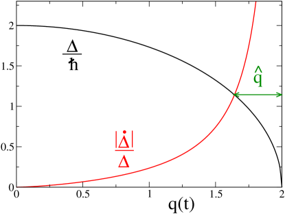
Figure 1: (color) Illustration of Eq. (12) in units of $\tau_{0}^{-1}$ (13) on the vertical axis. The plot is for $\tau_{Q}/\tau_{0}=1$.

$$\hat{q}\cong\frac{1}{4^{2/3}}\left(\frac{\tau_{0}}{\tau_{Q}}\right)^{2/3},\ \ \tau_{0}=\frac{\hbar}{n|c_{1}|}.$$ (13)

This, of course, corresponds to (3) with $z\nu=1/2$ and $\Delta_{0}=2n|c_{1}|$. A simple estimation of the constant $\tau_{0}$ by the peak density in the Berkeley experiment, $2.8\times 10^{14}cm^{-3}$, gives $\tau_{0}\approx 16ms$. In this section and Sec. IV all the results can be obtained without assuming any particular value of $\tau_{0}$.

Qualitatively, prediction (13) is in agreement with what we expect: the slower the quench is (the larger $\tau_{Q}$ is), the closer to the critical point the condensate can be driven adiabatically.

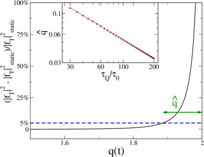
Figure 2: (color) Departures of the transverse magnetization from the static prediction during evolution in the broken-symmetry phase. $|f_{T}|^{2}_{\rm static}$ refers to the squared modulus of (8). We arbitrarily define that when these departures exceed $5\%$, the system leaves the adiabatic regime and starts the non-equilibrium dynamics (other reasonable thresholds $<10\%$ give the same scaling result). The inset shows the result of power law fit pointing to $\hat{q}=1.05\times(\tau_{0}/\tau_{Q})^{0.651\pm 0.001}$, which compares well to theoretical prediction (13). The fit is presented as a solid line, while numerics comes as pluses. Note the log-log scale on the inset. The fit was done for $\tau_{Q}/\tau_{0}=30\cdots 200$. The larger $\tau_{Q}$’s are taken to the fit, the closer scaling exponent approaches $2/3$. On the main plot we have a simulation for $\tau_{Q}/\tau_{0}=30$.

Quantitatively, solution (13) turns out to be remarkably accurate in the wide range of quench times $\tau_{Q}$ as depicted in Fig. 2. In that plot we define the instant $\hat{q}$ to be the distance from a critical point when the departure of system transverse magnetization from a static (ground state) prediction starts exceeding some threshold, e.g., $5\%$ of the instantaneous GS value. From the fit there we get that

$$\hat{q}=1.05\times\left(\frac{\tau_{0}}{\tau_{Q}}\right)^{0.651\pm 0.001}$$

in excellent agreement with (13) with respect to the scaling exponent. The prefactor, which obviously depends on the threshold used for the numerical determination of $\hat{q}$ is of the same order as in (13). Additional details are seen in Fig. 2. The error in the determination of the scaling exponent is one standard deviation coming from a linear fit on a log-log plot. All fitting errors in this paper are determined in this way.

Let’s look at the system magnetization at the critical point. To proceed further it is convenient to define the condensate energy density as

$$E=-\frac{|c_{1}|}{2}|f_{T}|^{2}+2n|c_{1}|q|\psi_{1}|^{2},$$ (14)

which is equal in the SMA to the contribution of the last two terms in Eq. (4) to the condensate energy per volume (the first two terms in Eq. (4) are unimportant in the SMA as the gradient term equals zero while the density-density interaction term $\sim c_{0}$ is a constant). In Fig. 3 we observe that $|f_{T}|^{2}\sim\tau_{Q}^{-2/3}$ and $E\sim\tau_{Q}^{-4/3}$. Putting these two scalings into Eq. (14) we see that

$$|\psi_{1}|^{2}=\frac{|f_{T}|^{2}}{8n}$$

at the critical point in the leading, i.e., $\tau_{Q}^{-2/3}$, order in the quench rate.

It is now interesting to ask whether there is any relation between the condensate magnetization at the point where the system goes out of equilibrium, $q=2-\hat{q}$, and the condensate magnetization at the critical point, $q=2$. The condensate magnetization at $q=2-\hat{q}$ equals (in the slow transition limit where $\hat{q}\ll 1$)

$$|f_{T}|^{2}/n^{2}=1-(2-\hat{q})^{2}/4\approx\hat{q}\sim\tau_{Q}^{-2/3}$$

so $|f_{T}(q=2-\hat{q})|^{2}$ scales with the quench rate in the same way as $|f_{T}(q=2)|^{2}$. This resembles the adiabatic-impulse simplification of dynamics bodzio ; dorner , where it is assumed that the evolution of a system undergoing a phase transition is either adiabatic or impulse, and the impulse stage implies no changes in the state of the system. Here this simple picture gives a correct scaling of the system magnetization at the critical point from the value of $\hat{q}$ – the location where the system leaves the adiabatic regime. This is a good approximation despite the fact that the condensate does not enter an ideal “impulse” regime. Indeed, the wave-function is not “frozen” and does change from $q=2-\hat{q}$ to $q=2$. Remarkably, however, these changes are such that instead of getting magnetization equal to $|f_{T}(q=2-\hat{q})|^{2}$ at the critical point (ideal impulse dynamics) we get $const\cdot|f_{T}(q=2-\hat{q})|^{2}$, where the constant is $\tau_{Q}$-independent. This character of condensate evolution toward a critical point is universal with respect to quench time. It is depicted in Fig. 4.

Now we would like to address how these critical scalings can be experimentally observed. One obvious way is to watch the condensate dynamics at different times as was done in the Berkeley experiment nature_kurn . Another approach involving interesting physics would be to stop a change of $q$ and watch subsequent magnetization dynamics. This approach will be discussed in the next section.

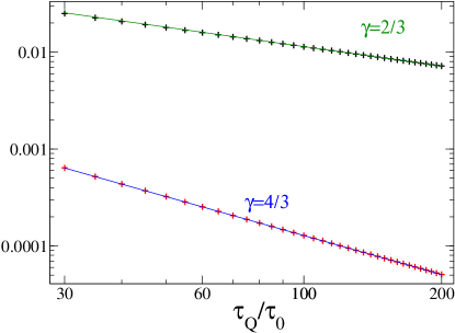
Figure 3: (color) Scaling of the condensate properties at the critical point. The upper data presents $|f_{T}|^{2}/n^{2}$, where $f_{T}$ is the transverse magnetization, while the lower data is for $E/n^{2}|c_{1}|$, where $E$ (energy density) is given by (14). The pluses come from numerics, while the solid lines present the curves $\sim(\tau_{0}/\tau_{Q})^{\gamma}$ with $\gamma=2/3$ ($4/3$) for the upper (lower) data. This confirms that at the critical point $|f_{T}|^{2}\sim\tau_{Q}^{-2/3}$, while $E\sim\tau_{Q}^{-4/3}$.

Figure 4: (color) Illustration of the scaling of departures of the condensate transverse magnetization, $|f_{T}|^{2}$, from the static prediction, $|f_{T}|^{2}_{\rm static}$, given by the squared modulus of (8). The solid black line is for $\tau_{Q}/\tau_{0}=30$, while red dots show data for $\tau_{Q}/\tau_{0}=60$. The plot shows that the departures of the transverse magnetization from a GS prediction near a critical point scale as $\tau_{Q}^{-2/3}$ after rescaling of the distance from the critical point, $2-q$, by a $\tau_{Q}^{2/3}$ factor.

IV Dynamics of magnetization after the quench

Suppose that one stops driving the system at some $q\geq 2$ and lets it evolve freely, which leads to magnetization oscillations. We would like to investigate here whether the information about the system excitation at the critical point can be extracted from the amplitude and/or period of these oscillations. In other words, we want to find out what are the signatures of the nonequilibrium dynamics in the broken-symmetry phase that may be observable in the polar phase. This problem is of both experimental and theoretical interest.

IV.1 Quench stops at the critical point

Suppose the condensate is driven from $q=0$ to the critical point with (10). The critical point is reached at $t=4\tau_{Q}$ and then $q(t\geq 4\tau_{Q})=2$, i.e., free (without any driving) evolution takes place. The evolution of magnetization for such a problem is presented in Fig. 5, where periodic oscillations are easily seen. Our aim is to describe them and show that both their amplitude and their period contain information on how the condensate was excited at the critical point.

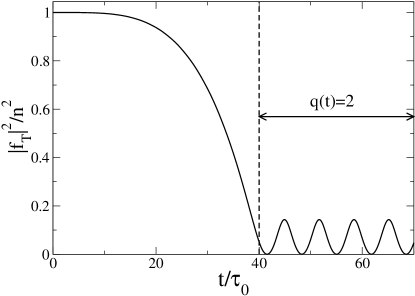
Figure 5: Time evolution of the magnetization during the quench that stops at the critical point. This plot is for $\tau_{Q}/\tau_{0}=10$. The critical point is reached at $t/\tau_{0}=4\tau_{Q}/\tau_{0}=40$, so $q(t\leq 40\tau_{0})$ is given by (10) while $q(t>40\tau_{0})=2$. The system excitation due to approaching the critical point is visible from the nonzero magnetization at $t/\tau_{0}\geq 40$: if the evolution would be adiabatic, the condensate magnetization at the critical point would be zero and no magnetization oscillations would be present on the plot.

In this case one can derive the following equation for the evolution of the magnetization:

$$\ddot{f}_{T}(t)=-\left(\frac{4|c_{1}|}{\hbar^{2}}E+2\frac{|c_{1}|^{2}}{\hbar^{2}}|f_{T}(t)|^{2}\right)f_{T}(t),$$ (15)

where $E$ is the system energy density (14) at the critical point (in fact, also at any other time since lack of parameter changes results in energy conservation). This equation can be obtained straightforwardly from Eqs. (6) and (II). It is an interesting equation: in the limit of slow transition, when the amplitude of oscillations becomes very small, the nonlinear term dominates the physics rather than being negligible compared to the $\sim E$ term promoting harmonic oscillations. Indeed, from Sec. III we see that $|c_{1}|E/|c_{1}|^{2}|f_{T}|^{2}\sim(\tau_{0}/\tau_{Q})^{2/3}\ll 1$ for slow enough quench.

The exact solution reads

$$f_{T}(t)=A\,{\rm cn}\left(\frac{|Ac_{1}|}{\hbar\kappa}t+\theta,\kappa\right),$$ (16)

where $\rm cn$ is the Jacobi cosine whittaker ,

$$\kappa=\sqrt{\frac{\alpha}{1+\alpha}}\frac{1}{\sqrt{2}},\ \ \alpha=\frac{|c_{1}|}{2E}|A|^{2},$$

and $A$ and $\theta$ are given by initial conditions. They both might be found from a fit to experimental data. In particular, $|A|^{2}$ is given by the amplitude of free $|f_{T}|^{2}$ oscillations, because the Jacobi cosine (16) oscillates periodically between $\pm 1$.

The Jacobi cosine was formerly used in the spin-1 condensate context in ferro_exp_jacobi ; cn . It is periodic – ${\rm cn}(x,\kappa)={\rm cn}(x+4K(\kappa),\kappa)$ – where $K(\kappa)$ is the complete elliptic integral of the first kind. In the time domain this periodicity translates into

$$\Delta t=4\kappa\left|\frac{\hbar}{Ac_{1}}\right|K(\kappa).$$ (17)

To simplify this expression we note that from the fact that the Jacobi cosine in (16) is bounded by $\pm 1$, $f_{T}$ and $A$ are of the same order and so we expect $|A|\sim\tau_{Q}^{-1/3}$. Moreover, as $E\sim\tau_{Q}^{-4/3}$ we get that in the limit of large $\tau_{Q}$ (slow transitions) $\alpha\sim(\tau_{Q}/\tau_{0})^{2/3}\gg 1$ and so $\kappa\to 1/\sqrt{2}$. This last result allows us to write

$$\Delta t=\frac{\Gamma(1/4)^{2}}{\sqrt{2\pi}}\left|\frac{\hbar}{Ac_{1}}\right|.$$ (18)

This finding is quite interesting: the periodicity is amplitude-dependent unlike in the harmonic oscillator case. This simple result predicting the inverse proportionality of the period and the amplitude of oscillations is accurate to about $1\%$ for experimentally relevant quenches as depicted in inset (a) of Fig. 6.

The numerical results on the oscillation period $\Delta t$ when the quench stops at $q=2$ are presented in Fig. 6. From the fit we see that $\Delta t$ scales as $\tau_{Q}^{1/3}$ in accordance with expression (18) supplemented with the above observation that $|A|\sim\tau_{Q}^{-1/3}$ (proven numerically in the inset (b) of Fig. 6).

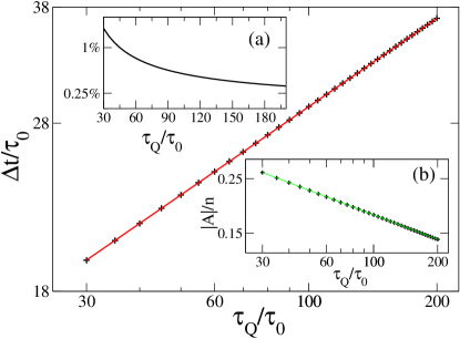
Figure 6: (color) Here we show the properties of the system when the change of $q$ stops at the critical point and then there is a free evolution going on. Note that there is a logarithmic scale on the vertical and horizontal axes of the main plot and the inset (b). Main plot: the periodicity interval $\Delta t$ of $f_{x,y}(t)$ during free oscillations. The fit (red line) to numerics (pluses) gives $\Delta t\sim\tau_{Q}^{0.3350\pm 0.0001}$. Inset (a): the difference between (18) and (17) divided by (17), i.e., relative departures of the approximate formula for oscillation period from the exact result. The approximate formula (18) overestimates the exact result by about one percent in a wide range of $\tau_{Q}/\tau_{0}$’s. Inset (b): dependence of $|A|$ from (16) on quench time $\tau_{Q}$. The fit (green line) to numerics (pluses) gives $|A|\sim\tau_{Q}^{-0.3304\pm 0.0001}$ in agreement with adiabatic - impulse simplification of the condensate dynamics.

IV.2 Quench stops after passing the critical point

According to our numerical simulations there are three stages of such evolution depicted in Fig. 7: (i) the system is driven to the critical point through the entire broken symmetry phase and its magnetization at the critical point scales as $|f_{T}|^{2}\sim\tau_{Q}^{-2/3}$ (only barely noticeable magnetization oscillations are present – see Ref. liniowe ); (ii) the condensate is driven by a change of $q$, Eq. (10), in the polar phase and we observe there damped magnetization oscillations; (iii) the free evolution after we stop ramping up $q(t)$ takes place and periodic magnetization oscillations appear. These oscillations are described by

$$\ddot{f}_{T}=-\left[\tau_{0}^{-2}q(q-2)+4\frac{|c_{1}|}{\hbar^{2}}E+2\frac{|c_{1}|^{2}}{\hbar^{2}}|f_{T}(t)|^{2}\right]f_{T},$$ (19)

where again $\dot{E}=0$ and Eqs. (6) and (II) have been employed in derivation of (19). The exact solution in terms of the Jacobi cosine function exists and has form (16) with

$$\alpha=\frac{|Ac_{1}|^{2}}{q(q-2)\hbar^{2}/2\tau_{0}^{2}+2E|c_{1}|}.$$

Now, in the limit of fixed $q>2$ and large $\tau_{Q}$ (slow transition) we have a different behavior of the Jacobi cosine than above. Namely, now $\alpha\sim(\tau_{0}/\tau_{Q})^{2/3}\ll 1$ which results in $\kappa\to 0$ and ${\rm cn(\bullet,\kappa)}\to\cos(\bullet)$. In this limit the last two terms in (19) can be neglected and the Jacobi cosine turns into a normal cosine function: harmonic oscillations show up with a repetition period

$$\Delta t=\frac{2\pi\tau_{0}}{\sqrt{q(q-2)}}.$$ (20)

Naturally, the transition between Jacobi cosine oscillations and typical harmonic dynamics is gradual and can be traced quantitatively with the exact solution (16). We can compare (20) to the numerics. For the evolutions where the increase of $q$ stops at $q=3$, as is the case in Fig. 7, we get from (20) that $\Delta t=2\times 1.814\tau_{0}$, while from numerics we obtain $2\times 1.804\tau_{0}$ for $\tau_{Q}/\tau_{0}=30$ and $2\times 1.812\tau_{0}$ for $\tau_{Q}/\tau_{0}=200$ (notice that $|f_{T}|^{2}$ oscillates with $1/2$ of the period (20) and so our numerical results extracted from $|f_{T}|^{2}$ oscillations were multiplied by a factor of two). As we see, the larger $\tau_{Q}$, the better the agreement because the nonlinear corrections become smaller. This is in fact bad news: as (20) is $\tau_{Q}$-independent, we can no longer use repetition period $\Delta t$ to investigate the dynamics of the quantum phase transition.

Fortunately, however, behavior of the amplitude of free magnetizations oscillations provides an easily visible signature of the non-equilibrium dynamics. As shown in the inset of Fig. 7, the amplitude of $|f_{T}|^{2}$ scales as $\tau_{Q}^{-1}$. This scaling results from two observations. First, the driving in the polar phase starting from $q=2$ and proceeding to $q\gtrsim 3$ damps the amplitude of $|f_{T}|^{2}$ by a factor of $\tau_{Q}^{-1/3}$. We have verified this numerically by simulating different evolutions that begin from a fixed, $\tau_{Q}$ independent, state. Second, the scaling of $|f_{T}|^{2}$ at the phase boundary is $\tau_{Q}^{-2/3}$. Combining these two results one easily justifies $\tau_{Q}^{-1}$ scaling from the numerics.

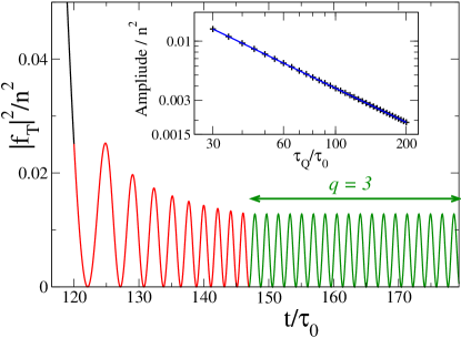
Figure 7: (color) Dynamics of the system driven by the change of $q(t)$ given by (10) until the point $q=3$, and then undergoing a free evolution with $q$ time independent. The main plot shows data for $\tau_{Q}/\tau_{0}=30$. The free evolution starts at $t/\tau_{0}=\sqrt{24}\tau_{Q}/\tau_{0}\approx 147$. Different stages of evolution are encoded in colors: black (evolution in broken-symmetry phase), red (dynamics in polar phase induced by change of $q$), green (free dynamics in the polar phase, $\dot{q}=0$). Inset: the scaling of the amplitude of $|f_{T}(t)|^{2}$ oscillations during free evolution at $q=3$ (depicted in green). Pluses come from numerics, while the line is the fit corresponding to $\sim\tau_{Q}^{-1.0013\pm 0.0001}$ scaling.

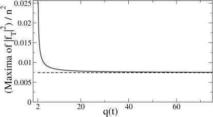
Figure 8: Maxima of the system magnetization, $|f_{T}|^{2}$, during an uninterrupted driving through the polar phase with $q(t)$ given by (10). The solid line comes from numerics and provides the upper envelope for oscillations of $|f_{T}(t)|^{2}$. The data is for one run with $\tau_{Q}/\tau_{0}=30$. The dashed line is the asymptotic (large $q$) value for the solid line. It is obtained from a linear fit $({\rm Maxima\ of\ }|f_{T}|^{2})/n^{2}=a+b\frac{1}{q}$ for $q\sim 100$ data. The fit gives $a\approx 0.0074$ plotted as a dashed line. Additionally, we have verified numerically, that for different $\tau_{Q}$’s the following scaling holds: $a\sim\tau_{Q}^{-1}$, which can be explained in the same way as the fitting result from the inset of Fig. 7.

Finally, we comment on what happens when the system is continuously driven through the polar phase. Combining Eqs. (6) and (II) one easily arrives at

$$\ddot{f}_{T}=-\tau_{0}^{-2}q(t)(q(t)-2)f_{T}-8\frac{n|c_{1}|^{2}}{\hbar^{2}}q(t)|\psi_{1}(t)|^{2}f_{T}+\frac{\dot{q}(t)}{q(t)}\dot{f}_{T},$$ (21)

that has to be solved with initial conditions given at instant $t_{i}$ by $f_{T}(t_{i})$ and $\dot{f}_{T}(t_{i})=iq\sqrt{2}\tau_{0}^{-1}(\psi_{1}^{*}\psi_{0}-\psi_{-1}\psi_{0}^{*})|_{t_{i}}$. Two remarks are in order. First, the same initial conditions apply to (15) and (19). Second, equation (21) is no longer self-consistent: an additional equation for $\psi_{1}(t)$ dynamics has to be solved simultaneously unless the term $\sim|\psi_{1}(t)|^{2}$ is negligible.

As we have observed in Fig. 7 the magnetization oscillations are damped when the system is driven in the polar phase. It turns out, however, that when we continue driving the condensate, the amplitude of magnetization oscillations reaches some nonzero asymptotic value, scaling as $\tau_{Q}^{-1}$, instead of decreasing to zero. This is supported by Fig. 8 and the following analysis. First, we assume that $q(t)\gg 2$ such that it is safe to approximate $q(t)(q(t)-2)$ by $q(t)^{2}$. Second, we neglect the second term in (21) as it is small compared to the first one in the slow transition limit. After that we end up with the following equation that can be solved exactly

$$\ddot{f}_{T}=-\tau_{0}^{-2}q(t)^{2}f_{T}+\frac{\dot{q}(t)}{q(t)}\dot{f}_{T}.$$ (22)

This is precisely a driven harmonic oscillator with anti-friction since $\dot{q}(t)/q(t)$ is positive in our case. In a classical mechanical picture we may imagine that (22) describes a particle in a harmonic potential under the influence of a force that acts along its velocity. Such a force fights the tendency to squeeze particle motion due to increase of the frequency of the harmonic oscillator. Interestingly, it turns out that the particle perfectly maintains the amplitude of its motion because the exact solution of (22), constrained by $\dot{\phi}=0$ from (II), is

$$f_{T}=C\cos\left(\frac{1}{\tau_{0}}\int dtq(t)+\theta\right),\ \ \dot{C}=0.$$

Additionally, we stress the fact that this solution is valid for any smooth $q(t)$ dependence and not just (10). In particular, in the opposite limit when $q(t)$ decreases in time the “anti-friction” term works as a special friction term that slows the particle down so that it oscillates with constant amplitude instead of spreading out.

This phenomenon can be qualitatively explained as follows. As it happens at $q(t)\gg 2$ we can safely assume that the magnon modes of the system do not become excited any more during driving. This is so because they have energy gap that becomes large far away from the critical point. These modes are responsible for the scattering of atoms between $m=0$ and $m=\pm 1$ condensate components ueda_spectrum . In the absence of that process the populations of $m=0,\pm 1$ sublevels should be constant, which implies that

$$|f_{T}|^{2}=8|\psi_{1}|^{2}|\psi_{0}|^{2}\cos^{2}\left(\chi_{0}-\frac{\chi_{1}+\chi_{-1}}{2}\right)$$

will undergo fixed amplitude oscillations induced by rotation of the condensate phases.

V Dynamics in a slightly inhomogeneous system

In this section we would like to compare the results obtained from a Single Mode Approximation enforcing the translational symmetry onto wave-function of the system to the more experimentally relevant inhomogeneous (“disordered”) problem. To this aim we assume that the atom cloud is placed in a box-like trap and impose density and phase fluctuations onto it. These may come from experimental imperfections and quantum fluctuations.

The results presented here come from numerics done in a one-dimensional configuration and so we present an explicitly 1D description below unless stated otherwise. We consider untrapped system: atoms in the box as in the experiment raizen done with spinless bosons. We estimate the parameters for these 1D simulations as in ferro_bodzio taking into account the experimental setup of nature_kurn . Below $L\approx 400\mu m$ is the size of the box keeping $N=2\times 10^{6}$ atoms confined along the $z$ direction.

We introduce disorder by modifying the initial wave function at $q(t=0)=0$ in the following way:

$$\Psi\approx\sqrt{n}\left(\begin{array}[]{c}\frac{1}{2}\phi_{1}(z)e^{i\chi_{1}}\\ \frac{1}{\sqrt{2}}\phi_{0}(z)e^{i(\chi_{1}+\chi_{-1})/2}\\ \frac{1}{2}\phi_{-1}(z)e^{i\chi_{-1}}\end{array}\right),\ \int_{0}^{L}dz|\Psi|^{2}=N,$$

where the mode amplitude is proportional to:

$$\phi_{m}=\sqrt{1+\delta\sum_{n=1}^{\kappa}e^{i\eta_{n}^{(m)}}r_{n}^{(m)}\exp\left(-\frac{(z-z_{n}^{(m)})^{2}}{\sigma^{2}}\right)}.$$ (23)

There $\delta$ gives the strength of the disorder, $\eta^{(m)}_{n},\chi_{\pm 1}\in[0,2\pi)$ are random phases, $r_{n}^{(m)}\in[0,1]$ are random amplitudes, and $z_{n}^{(m)}\in[0,L]$ are random positions of gaussian disturbances. All these parameters are generated with uniform probability density. We have chosen $\sigma$ to be equal to the spin healing length $\xi_{s}$ and assumed that the average spacing between Gaussian perturbations is $2\xi_{s}$. The spin healing length in the experiment nature_kurn is $2.4\mu m$, so that $\kappa$, the number of Gaussians in (23), is about $80$ ($L/2\xi_{s}$). The meaning of $\delta$ is that it provides a characteristic relative-to-background size of density variations. A typical disordered pattern in (23) is depicted in Fig. 9. Now our goal is to answer what is the range of the $\delta$ parameter that allows for observation of qualitatively the same physics as in the homogeneous system described in Secs. III and IV.

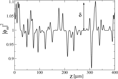
Figure 9: Plot of $|\phi_{m}(z)|^{2}$ for a typical realization of disorder (23). The parameter $\delta=10\%$.

To look at the dynamics in the broken-symmetry phase, we have done calculations for different $\delta\in(0,0.2)$. For each $\delta$ we randomly generate many-times the pattern (23) and evolve the system to the critical point at different quench times $\tau_{Q}$. The patterns are independently generated for every evolution, which shall resemble the experimental situation where the structure of “imperfections” fluctuates from run to run. Then for each pair $(\delta,\tau_{Q})$ we average the mean system magnetization over $N_{r}=30$ runs,

$$\langle|f_{T}|^{2}\rangle=\frac{1}{N_{r}}\sum_{i=1}^{N_{r}}\frac{1}{L}\int_{0}^{L}dz|f_{T}^{(i)}(z,t)|^{2},$$

where $f_{T}^{(i)}(z,t)$ is the condensate transverse magnetization in the $i$-th run.

We look at two quantities: the distance $\hat{q}(\tau_{Q})$ from the critical point where the system starts the non-adiabatic evolution due to approaching the critical point, and the scaling of the condensate magnetization at the critical point. Both are defined in the same way as in Sec. III except that now we use $\langle|f_{T}|^{2}\rangle$ instead of $|f_{T}|^{2}$. Our results suggest that the scaling exponents in the disordered system can match the SMA predictions within a few percent accuracy for $\delta\lesssim 2\%$. Quantitatively, as we see in Table 1, the scaling exponent $\lambda$ given by $\hat{q}\sim\tau_{Q}^{-\lambda}$ stays reasonably close to the $2/3$ value for the homogeneous system for $\delta$ as large as $3\%$. For larger $\delta$, e.g., $\delta=5\%$ the numerical data clearly departs from the power law. The scaling exponent $\sigma$, defined at the critical point as $\langle|f_{T}|^{2}\rangle\sim\tau_{Q}^{-\sigma}$, deviates noticeably from the SMA prediction already for $\delta=2\%$ (Table 1). For larger $\delta$, e.g., $\delta=3\%$ numerics does not follow the power law anymore.

	$\lambda$	$\sigma$
$\delta=0.5\%$	$0.65\pm 0.01$	$0.650\pm 0.001$
$\delta=1\%$	$0.67\pm 0.01$	$0.647\pm 0.001$
$\delta=2\%$	$0.65\pm 0.01$	$0.60\pm 0.02$
$\delta=3\%$	$0.64\pm 0.02$

Table 1: The scaling exponents $\lambda$, $\hat{q}\sim\tau_{Q}^{-\lambda}$, and $\sigma$, $\langle|f_{T}|^{2}\rangle$ at the critical point $\sim\tau_{Q}^{-\sigma}$. The values and errors (one standard deviation) come from a linear fit on a log-log plot to data in the range of $\tau_{Q}=74ms\cdots 1.1s$. The Single Mode Approximation ($\delta=0$) points to $\lambda,\sigma\approx 2/3$. The definition of $\hat{q}$ is the same as in Fig. 2 except $\langle|f_{T}|^{2}\rangle$ is used instead of $|f_{T}|^{2}$.

There are at least two reasons for discrepancies between disordered and homogeneous results. First and most importantly, the presence of disorder perturbs magnetization affecting determination of both exponents from Table 1. Even when these departures from a GS are relatively small compared to the GS magnetization when the system starts time evolution at $q=0$, they can be significant when compared to the condensate magnetization close to or at the critical point where scaling exponents are determined. Second, our prediction of the scaling exponents is based on translationally invariant theory, i.e., momentum $k=0$ problem, while the introduction of disorder leads to population of $k\neq 0$ modes. A more involved description with the gap $\Delta$ (11) being a function of $k$ should be used when the population of $k\neq 0$ modes becomes significant.

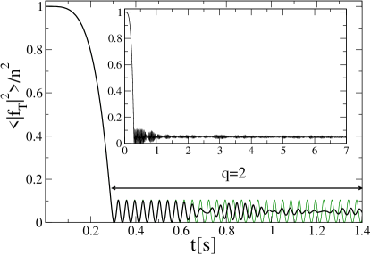
Figure 10: (color) Dynamics of the transverse magnetization in the inhomogeneous system during a quench with $\tau_{Q}=74ms$. The change of $q(t)$ stops at the critical point: $q(t\geq 4\tau_{Q}\approx 0.3s)=2$. The thick black line is for $\delta=1\%$. The thin green line presents $\delta=0$ result, i.e., the Single Mode Approximation outcome. The inset shows long time behavior of the black thick curve from the main plot. The initial state for that evolution is the same as in Fig. 11.

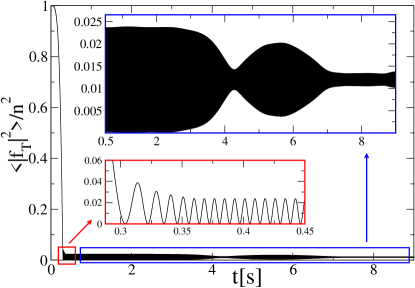
Figure 11: (color) Dynamics of the transverse magnetization in the inhomogeneous system during a quench with $\tau_{Q}=74ms$. The change of $q(t)$ stops at $3$ in the polar phase, $q(t\geq\sqrt{24}\tau_{Q}\approx 0.36s)=3$, and $\delta=1\%$. The insets show enlarged data from the main plot corresponding to the regions depicted with boxes. The period of oscillations is so small that individual oscillations are not resolved in the main plot and the upper inset. The lower inset does not show the SMA result as it is practically indistinguishable from the inhomogeneous calculation. Arrows indicate which inset belongs to what box. The initial state for that evolution is the same as in Fig. 10.

Now we would like to look at the system dynamics in the polar phase. In Sec. IV we have observed that the transverse magnetization undergoes periodic oscillations in a homogeneous problem after stop of driving. Now we see dephasing dynamics spoiling this picture after a time inversely proportional to the disorder magnitude and the quench time $\tau_{Q}$. The latter observation results from the fact that the slower we go at fixed $\delta$, the more significant the disorder is compared to the system magnetization in the polar phase.

Fig. 10 presents the evolution with $\tau_{Q}=74ms$ and $\delta=1\%$. The change of $q$ stops at the critical point there. For these parameters the scaling exponents are very close to the Single Mode Approximation result (see Table 1). As is illustrated in Fig. 10, however, dephasing takes place after about $7-9$ oscillations. To observe more magnetization oscillations closely following the SMA result, for twice that time, $\delta$ has to be about one order of magnitude smaller. Therefore, the system dynamics is quite sensitive to inhomogeneities when the condensate is left at the critical point. This should result from the coupling between different $k$ modes due to nonlinear terms in the evolution equation.

Fig. 11 presents the evolution where driving stops at $q=3$ (similarly as in Fig. 7). The parameters and the initial state taken for this simulation are the same as in Fig. 10. This time the undriven dynamics takes place in the regime where nonlinear couplings are small. As a result, the dephasing occurs after hundreds of oscillations even though the disorder amplitude, $\delta=1\%$, is the same as in Fig. 10.

To explain dephasing when the evolution stops away from a critical point, we can linearize the coupled Gross-Pitaevskii equations. Below we do it in an explicitly 3D configuration to use the same notation as in Secs. III and IV (the 1D result is qualitatively the same). We assume that

$$\Psi=\sqrt{n}\left(\begin{array}[]{c}\delta\psi_{1}({\bf r},t)\\ 1+\delta\psi_{0}({\bf r},t)\\ \delta\psi_{-1}({\bf r},t)\end{array}\right)\exp\left(-i\frac{\mu}{\hbar}t\right)$$

where the chemical potential is $\mu=nc_{0}$, $|\delta\psi_{m}|\ll 1$, and $\int d{\bf r}(\delta\psi_{0}+\delta\psi_{0}^{*})\equiv 0$ to keep $\int d{\bf r}\Psi^{\dagger}\Psi=N+O(\delta\psi^{2}_{m})$. In leading order

$$f_{T}=\sqrt{2}n(\delta\psi^{*}_{1}+\delta\psi_{-1}),$$

and its dynamics at fixed $q$ is given by

$$\ddot{f}_{T}=-\frac{\hbar^{2}}{4M^{2}}\nabla^{4}f_{T}+(q-1)\frac{n|c_{1}|}{M}\nabla^{2}f_{T}-\tau_{0}^{-2}q(q-2)f_{T},$$

where the last term is known from (19). That can be solved by the substitution $f_{T}\sim\cos({\bf kr}-\omega(k)t)$, giving

$$\hbar\omega(k)=\sqrt{\epsilon_{k}^{2}+\epsilon_{k}2(q-1)n|c_{1}|+n^{2}|c_{1}|^{2}q(q-2)},$$

where $\epsilon_{k}=\hbar^{2}k^{2}/2M$. When disorder is present, different $k$ modes will be occupied and they will oscillate at different frequencies $\omega(k)$, which will result in the dephasing observed in Fig. 11. The expression for $\omega(k)$ shall not be used at $q=2$, where linearized theory fails as was shown within the SMA in Sec. IV.

VI Summary

We have analyzed transitions from the broken-symmetry phase to the polar phase occurring on the finite timescale $\tau_{Q}$. Our focus was on slow transitions, when the condensate goes out of equilibrium near a critical point. We have presented a simple theory predicting that the evolution will cease to be adiabatic before reaching the polar phase at the distance $\sim\tau_{Q}^{-2/3}$ from the critical point. This result was found to be in excellent agreement with numerics. Applying the basic assumptions of the adiabatic-impulse approach dorner ; bodzio , which originates from the Kibble-Zurek theory of nonequilibrium dynamics of classical phase transitions kibble ; zurek , we have explained why the transverse magnetization of the condensate driven to the critical point scales as $\tau_{Q}^{-2/3}$ as well. Subsequently we have analyzed how the latter result can be experimentally extracted from the observation of magnetization oscillations. Three cases were considered. First, we have studied what happens when the quench stops at the critical point and the system follows free evolution. It was shown that the periodic oscillations appear with the repetition period coupled to the amplitude of transverse magnetization oscillations. The repetition period was found to scale as $\tau_{Q}^{1/3}$, where the exponent was directly related to the scaling of the transverse magnetization at the critical point. That nonlinear dynamics was exactly described within the mean-field approach in terms of Jacobi elliptic functions. Second, we have studied what happens when the system is driven into the polar phase, and then undergoes a free evolution. In that case we have shown that its excitation at the critical point can be easily extracted from the scaling of the amplitude of the free magnetization oscillations given by $\tau_{Q}^{-1}$. Third, we have studied what happens when the condensate is driven without any interruptions not only in the broken-symmetry phase, but also in the polar phase. In this case the amplitude of driven magnetization oscillations reaches a non-zero asymptotic value: the condensate magnetization is described as an unusual harmonic oscillator with anti-friction term that perfectly cancels the squeezing induced by the increase of the harmonic oscillator frequency.

All the above results were obtained within a translationally invariant Single Mode Approximation whose range of applicability was determined by introducing a controlled disorder into an initial wave function. We have found out that the amount of disorder has to be quite small to have the homogeneous system predictions applicable.

Future extensions of this work will include studies of quantum phase transitions dynamics in a harmonically trapped ferromagnetic condensate and investigations of the role of quantum fluctuations on the condensate dynamics.

VII Acknowledgments

We gratefully acknowledge the support of the U.S. Department of Energy through the LANL/LDRD Program for this work.

References

- (1) T.W.B. Kibble, J. Phys. A 9, 1387 (1976); Phys. Rep. 67, 183 (1980).
- (2) W.H. Zurek, Nature (London) 317, 505 (1985); Acta Phys. Pol. B 24, 1301 (1993); Phys. Rep. 276, 177 (1996).
- (3) W.H. Zurek, U. Dorner, and P. Zoller, Phys. Rev. Lett. 95, 105701 (2005).
- (4) J. Dziarmaga, Phys. Rev. Lett. 95, 245701 (2005); R.W. Cherng and L.S. Levitov, Phys. Rev. A 73, 043614 (2006); L. Cincio, J. Dziarmaga, M. M. Rams, and W. H. Zurek, Phys. Rev. A 75, 052321 (2007); P. Calabrese and J. Cardy, J. Stat. Mech. P06008 (2007); A. Fubini, G. Falci, and A. Osterloh, New J. Phys. 9, 134 (2007); V. Mukherjee, U. Divakaran, A. Dutta, and D. Sen, Phys. Rev. B 76, 174303 (2007); T. Caneva, R. Fazio, and G.E. Santoro, Phys. Rev. B 76, 144427 (2007).
- (5) B. Damski, Phys. Rev. Lett. 95, 035701 (2005); B. Damski and W.H. Zurek, Phys. Rev. A 73, 063405 (2006).
- (6) A. Polkovnikov, Phys. Rev. B 72, 161201(R) (2005).
- (7) I. Chuang et al., Science 251, 1336 (1991); M.J. Bowick et al., ibid. 263, 943 (1994); C. Bauerle et al., Nature (London) 382, 332 (1996); V.M.H. Ruutu et al., ibid. 382, 334 (1996); A. Maniv, E. Polturak, and G. Koren, Phys. Rev. Lett. 91, 197001 (2003); S. Ducci et al., ibid. 83, 5210 (1999); R. Monaco et al., ibid. 96, 180604 (2006); S. Casado et al., Eur. Phys. J. Special Topics 146, 87 (2007).
- (8) D.R. Scherer, C.N. Weiler, T.W. Neely, and B. P. Anderson, Phys. Rev. Lett. 98, 110402 (2007).
- (9) T.W.B. Kibble, Physics Today 60, 47 (2007).
- (10) T.-L. Ho, Phys. Rev. Lett. 81, 742 (1998); T. Ohmi and K. Machida, J. Phys. Soc. Jpn. 67, 1822 (1998); D.M. Stamper-Kurn and W. Ketterle, in Coherent Atomic Matter Waves, Proceedings of the Les Houches Summer School, Course LXXII, 1999, edited by R. Kaiser, C. Westbrook and F. David (Springer, New York, 2001).
- (11) L.E. Sadler, J.M. Higbie, S.R. Leslie, M. Vengalattore, and D.M. Stamper-Kurn, Nature (London) 443, 312 (2006).
- (12) J. Kronjäger, C. Becker, M. Brinkmann, R. Walser, P. Navez, K. Bongs, and K. Sengstock; M.-S. Chang, Q. Qin, W. Zhang, L. You, and M.S. Chapman, Nature Physics 1, 111 (2005).
- (13) L. Santos and T. Pfau, Phys. Rev. Lett. 96, 190404 (2006).
- (14) H. Saito, Y. Kawaguchi, and M. Ueda, Phys. Rev. A 75, 013621 (2007).
- (15) A. Lamacraft, Phys. Rev. Lett. 98, 160404 (2007).
- (16) M. Uhlmann, R. Schützhold, and U.R. Fischer, Phys. Rev. Lett. 99, 120407 (2007).
- (17) B. Damski and W.H. Zurek, Phys. Rev. Lett. 99, 130402 (2007).
- (18) H. Saito, Y. Kawaguchi, and M. Ueda, Phys. Rev. A 76, 043613 (2007).
- (19) G.I. Mias, N.R. Cooper, and S.M. Girvin, Phys. Rev. A 77, 023616 (2008).
- (20) S. Sachdev, Quantum Phase Transitions (Cambridge University Press, Cambridge UK, 2001).
- (21) K. Murata, H. Saito, and M. Ueda, Phys. Rev. A 75, 013607 (2007).
- (22) It is instructive here to note that after the rescaling and , where is defined in Eq. (13), we arrive at dimensionless description where none of the following quantities explicitly appears: , , , . Therefore, as long as the SMA is used, all the results are obtained without specifying the system-dependent parameters , , .
- (23) By choosing magnetic field strength one gets . In this case, however, the system gets slightly excited right at the start of the evolution as a result of a fairly abrupt switch of (e.g., ). As a result, the magnetization noticeably oscillates around the ground state prediction in the entire broken-symmetry phase for intermediate quench rates. The same effect shows up for (10), but to much smaller extent.
- (24) E.T. Whittaker and G.N. Watson, A Course of Modern Analysis, Sec. XXII of Fourth Edition (Cambridge University Press, Cambridge, 2003).
- (25) W. Zhang, D.L. Zhou, M.-S. Chang, M.S. Chapman, and L. You, Phys. Rev. A 72, 013602 (2005).
- (26) T.P. Meyrath, F. Schreck, J.L. Hanssen, C.-S. Chuu, and M.G. Raizen, Phys. Rev. A 71, 041604(R) (2005).