1 Introduction

Models of intersecting branes (see [1] for an overview) have been under an intense theoretical scrutiny in the last several years. The motivations for studying this class of theories are manifolds, being them obtained from special vacua of string theory, for instance from the orientifold construction [2, 3, 4]. Their generic gauge structure is of the form $SU(3)\times SU(2)\times U(1)_{Y}\times U(1)^{p}$, where the symmetry of the Standard Model (SM) is enlarged with a certain number of extra abelian factors $(p)$. Several phenomenological studies [5, 6, 7, 8, 9, 10] have allowed to characterize their general structure, whose string origin has been analyzed at an increasing level of detail [11, 12] down to more direct issues, connected with their realization as viable theories beyond the SM. Related studies of the Stückelberg field [13] in a non-anomalous context have clarified this mechanism of mass generation and analyzed some of its implications at colliders both in the SM and in its supersymmetric extensions.

In scenarios with extra dimensions where the interplay between anomaly cancellations in the bulk and on the boundary branes is critical for their consistency, very similar models could be obtained following the construction of [14], with a suitable generalization in order to generate at low energy a non abelian gauge structure.

Specifically, the role played by the extra $U(1)$’s at low energy in theories of this type after electroweak symmetry breaking has been addressed in [5, 6, 7], where some of the quantum features of their effective action have been clarified. These, for instance, concern the phases of these models, from their defining phase, the Stückelberg phase, being the anomalous $U(1)$ broken at low energy but with a gauge symmetry restored by shifting (Stückelberg) axions, down to the electroweak phase - or Higgs-Stückelberg phase, (HS) - where the vev’s of the Higgs of the SM combine with the Stückelberg axions to produce a physical axion [5] and a certain number of goldstone modes. The axion in the low energy effective action is interesting both for collider physics and for cosmology [8], working as a modified Peccei-Quinn (PQ) axion. In this respect some interesting proposals to explain an anomaly in gamma ray propagation as seen by MAGIC [15] using a pseudoscalar (axion-like) has been presented recently, while more experimental searches of effects of this type are planned for the future by several collaborations using Cerenkov telescopes (see [15] for more details and references). Other interesting revisitations of the traditional Weinberg-Wilczek axion [16] to evade the astrophysical constraints and in the context of Grand Unification/mirror worlds [17] may well deserve attention in the future and be analyzed within the framework that we outline below. At the same time, comparisons between anomalous and non anomalous string constructions of models with extra $Z^{\prime}$s should also be part of this analysis [18].

The presence of axion-like particles in effective theories is, in general, connected to an anomalous gauge structure, but for reasons which may be rather different and completely unrelated, as discussed in [8]. For the rest, though, the study of the perturbative expansion in theories of this type is rather general and shows some interesting features that deserve a careful analysis. In [6, 7] several steps in the analysis of the perturbative expansion have been performed. In particular it has been shown how to organize the loop expansion in a gauge-invariant way in $1/M_{1}$, where $M_{1}$ is the Stückelberg mass. A way to address this point is to use a typical $R_{\xi}$ gauge and follow the pattern of cancellation of the gauge parameter in order to characterize it. This has been done up to 3-loop level in a simple $U(1)\times U(1)$ model where one of the two $U(1)$’s is anomalous.

The Stückelberg symmetry is responsible for rendering the anomalous gauge bosons massive (with a mass $M_{1}$) before electroweak symmetry breaking. A second scale $M$ controls the interaction of the axions with the gauge fields but is related to the first by a condition of gauge invariance in the effective action [8]. In general, for a theory with several $U(1)$’s, there is an independent mass scale for each Stückelberg field.

In the case of a complete extension of the SM incorporating anomalous $U(1)$’s, all the neutral current sectors, except for the photon current, acquire an anomalous contribution that modifies the trilinear (chiral) gauge interactions. For the $Z$ gauge boson this anomalous component decouples as $M_{1}$ gets large, though it remains unspecified. For instance, in theories containing extra dimensions it could even be of the order of 10 TeV’s or so, in general being of the order of $1/R$, where $R$ is the radius of compactification. In other constructions [4] based on toroidal compactifications with branes wrapping around the extra dimensions, their masses and couplings are expressed in terms of a string scale $M_{s}$ and of the integers characterizing the wrappings [9]. Beside the presence of the extra neutral currents, which are common to all the models with extra abelian gauge structures, here, in addition, the presence of chiral anomalies leaves some of the trilinear interactions to contribute even in the massless fermion (chiral) limit, a feature which is completely absent in the SM, since in the chiral limit these vertices vanish.

As we are going to see, the analysis of these vertices is quite delicate, since their behaviour is essentially controlled by the mass differences within a given fermion generation [7], and for this reason they are sensitive both to spontaneous and to chiral symmetry breaking. The combined role played by these sources of breaking is not unexpected, since any pseudoscalar induced in an anomalous theory feels both the structure of the QCD vacuum and of the electroweak sector, as in the case of the Peccei-Quinn (PQ) axion. In this work we are going to proceed with a general analysis of these vertices, extending the discussion in [7]. Our analysis here is performed at a field theory level, leaving the phenomenological discussion to a companion work. Our analysis is organized as follows.

After a brief summary on the structure of the effective action, which has been included to make our treatment self-contained, we analyze the Slavnov-Taylor identities of the theory, focusing our attention on the trilinear gauge boson vertices. Then we characterize the structure of the $Z\gamma\gamma$ and $ZZ\gamma$ vertices away from the chiral limit, extending the discussion presented in [7]. In particular we clarify when the CS terms can be absorbed by a re-distribution of the anomaly before moving away from the chiral limit. In models containing several anomalous $U(1)$’s different theories are identified by the different partial anomalies associated to the trilinear gauge interactions involving at least three extra $Z^{\prime}$s. In this case the CS terms are genuine components which are specific for a given model and are accompanied by a specific set of axion counterterms. Symmetric distributions of the partial anomalies are sufficient to exclude all the CS terms, but these particular assignments may not be general enough.

Away from the chiral limit, we show how the mass dependence of the vertices is affected by the external Ward identity, which is a generic feature of anomalous interactions for nonzero fermion masses. This point is worked out using chiral projectors and counting the mass insertions into each vertex. On the basis of this study we are able to formulate general and simple rules which allow to handle quite straightforwardly all the vertices of the theory. We conclude with some phenomenological comments concerning the possibility of future studies of these theories at the LHC. In an appendix we present the Faddeev-Popov lagrangean of the model, which has not been given before, and that can be useful for further studies of these theories.

1.1 Construction of the effective action

The construction of the effective action, from the field theory point of view, proceeds as follows [5, 7].

One introduces a set of counterterms in the form of CS and WZ operators and requires that the effective action is gauge invariant at 1-loop. Each anomalous $U(1)$ is accompanied by an axion, and every gauge variation of the anomalous gauge field can be cancelled by the corresponding WZ term. The remaining anomalous gauge variations are cancelled by CS counterterms. A list of typical vertices and counterterms is shown in Fig. 1.

Figure 1: Counterterms allowed in the low energy effective action in the chiral limit: anomalous contributions (A), CS interaction (B), WZ term (C) and $B-b$ mixing contribution (D). In particular the bilinear mixing of the axions with the gauge fields is vanishing only for on-shell vertices and is removed in the $R_{\xi}$ gauge in the WZ case. A discussion of this term and its role in the GS mechanism can be found in [20].

We consider the simplest anomalous extension of the SM with a gauge structure of the form $SU(3)\times SU(2)\times U(1)_{Y}\times U(1)_{B}$ model with a single anomalous $U(1)_{B}$. The anomalous contributions are those involving the $B$ gauge boson and involve the trilinear (triangle) vertices $BBB$, $BYY,$ $BBY,$ $BWW$ and $BGG$, where $W$’s and the $G$’s are the $SU(2)$ and $SU(3)$ gauge bosons respectively. All the remaining trilinear interactions mediated by fermions are anomaly-free and therefore vanish in the massless limit. Therefore the axion ($b$) associated to $B$ appears in abelian counterterms of the form $bF_{B}\wedge F_{B},bF_{B}\wedge F_{Y},bF_{Y}\wedge F_{Y}$ and in the analogous non-abelian ones $bTrW\wedge W$ and $bTrG\wedge G$. In the absence of a kinetic term for the axion $b$, its role is unclear: it allows to “cancel” the anomaly but can be gauged away. As emphasized by Preskill [19], the role of the WZ term is, at this stage, just to allow a consistent power counting in the perturbative expansion, hinting that an anomalous theory is non-renormalizable, but, for the rest, unitary below a certain scale. Theories of this type are in fact characterized by a unitarity bound since local a counterterm is not sufficient to erase the bad high energy behaviour of the anomaly [20]. Although the structure of the vertices constructed in this work is identified using the WZ effective action at the lowest order (using only the axion counterterm), their extension to the Green-Schwarz case is straightforward. In this second case the vertices here defined need to be modified with the addition of extra massless poles on the external gauge lines.

The b field remains unphysical even in the presence of a Stückelberg mass term for the B field, $\sim(\partial b-MB)^{2}$ since the gauge freedom remains and it is then natural to interpret $b$ as a Nambu-Goldstone mode. In a physical gauge it can be set to vanish.

Things change drastically when the B field mixes with the other scalars of the Higgs sector of the theory. In this case a linear combination of $b$ and the remaining CP-odd phases (goldstones) of the Higgs doublets becomes physical and is called the axi-Higgs. This happens only in specific potentials characterized also by a global $U(1)_{PQ}$ symmetry ($V_{PQ}$) [5] which are, however, sufficiently general. In the absence of Higgs-axion mixing the CP odd goldstone modes of the broken theory, after electroweak symmetry breaking, are just linear combinations of the Stückelberg and of the goldstone mode of the Higgs potential and no physical axion appears in the spectrum. For potentials that allow a physical axion, even in the massless case, the axion mass can be lifted by the QCD vacuum due to instanton effects exactly as for the Peccei-Quinn axion, but now the spectrum allows an axion-like particle.

1.2 Anomaly cancellation in the interaction eigenstate basis, CS terms and regularizations

The anomalies of the model are cancelled in the interaction eigenstate basis of $(b,A_{Y},B,W)$ and the CS and WZ terms are fixed at this stage. The B field is massive and mixes with the axion, but the gauge symmetry is still intact. The Ward identities of the theory for the triangle diagrams assume a nontrivial form due to the $B\partial b$ mixing. In the case of on-shell trilinear vertices one can show that these mixing terms vanish.

The CS counterterms are necessary in order to cancel the gauge variations of the $Y,W$ and $G$ gauge bosons in anomalous diagrams involving the interaction with $B$. These are the diagrams mentioned before. The role of these terms is to render vector-like at 1-loop all the currents which become anomalous in the interaction with the $B$ gauge boson. For instance, in a triangle such as $YBB$, the $A_{Y}B\wedge F_{B}$ CS term effectively “moves” the chiral projector from the Y vertex to the B vertex symmetrically on the two B’s, assigning the anomalies to the B vertices. These will then be cancelled by the axion $b$ via a suitable WZ term ($bF_{B}\wedge F_{Y}$).

The effective action has the structure given by

$${\mathcal{S}} = {\mathcal{S}}_{0}+{\mathcal{S}}_{an}+{\mathcal{S}}_{WZ}+{\mathcal{S}}_{CS}$$ (1)

where ${\mathcal{S}}_{0}$ is the classical action. It is a canonical gauge theory with dimension-4 operators whose explicit structure can be found in [7]. In Eq. (1) the anomalous contributions coming from the 1-loop triangle diagrams involving abelian and non-abelian gauge interactions are summarized by the expression

$${\mathcal{S}}_{an} = \frac{1}{2!}\langle T_{BWW}BWW\rangle+\frac{1}{2!}\langle T_{BGG}BGG\rangle+\frac{1}{3!}\langle T_{BBB}BBB\rangle$$ (2)

$$+\frac{1}{2!}\langle T_{BYY}BYY\rangle+\frac{1}{2!}\langle T_{YBB}YBB\rangle,$$

where the symbols $\langle\rangle$ denote integration [6]. In the same notations the Wess Zumino (WZ) counterterms are given by

$${\mathcal{S}}_{WZ} = \frac{C_{BB}}{M}\langle bF_{B}\wedge F_{B}\rangle+\frac{C_{YY}}{M}\langle bF_{Y}\wedge F_{Y}\rangle+\frac{C_{YB}}{M}\langle bF_{Y}\wedge F_{B}\rangle$$ (3)

$$+\frac{F}{M}\langle bTr[F^{W}\wedge F^{W}]\rangle+\frac{D}{M}\langle bTr[F^{G}\wedge F^{G}]\rangle,$$

and the gauge dependent CS abelian and non abelian counterterms [12] needed to cancel the mixed anomalies involving a B line with any other gauge interaction of the SM take the form

$${\mathcal{S}}_{CS} = +d_{1}\langle BY\wedge F_{Y}\rangle+d_{2}\langle YB\wedge F_{B}\rangle$$ (4)

$$+c_{1}\langle\epsilon^{\mu\nu\rho\sigma}B_{\mu}C^{SU(2)}_{\nu\rho\sigma}\rangle+c_{2}\langle\epsilon^{\mu\nu\rho\sigma}B_{\mu}C^{SU(3)}_{\nu\rho\sigma}\rangle.$$

Explicitly

$$\langle T_{BWW}BWW\rangle \equiv \int dx\,dy\,dzT^{\lambda\mu\nu,ij}_{BWW}(z,x,y)B^{\lambda}(z)W^{\mu}_{i}(x)W^{\nu}_{j}(y)$$ (5)

and so on.

The non-abelian CS forms are given by

$$C^{SU(2)}_{\mu\nu\rho} = \frac{1}{6}\left[W^{i}_{\mu}\left(F^{W}_{i,\,\nu\rho}+\frac{1}{3}\,g_{2}\,\varepsilon^{ijk}W^{j}_{\nu}W^{k}_{\rho}\right)+cyclic\right],$$ (6)

$$C^{SU(3)}_{\mu\nu\rho} = \frac{1}{6}\left[G^{a}_{\mu}\left(F^{G}_{a,\,\nu\rho}+\frac{1}{3}\,g_{3}\,f^{abc}G^{b}_{\nu}G^{c}_{\rho}\right)+cyclic\right].$$ (7)

In our conventions, the field strengths are defined as

$$F^{W}_{i,\,\mu\nu} = \partial_{\mu}W^{i}_{\nu}-\partial_{\nu}W^{i}_{\mu}-g_{2}\varepsilon_{ijk}W^{j}_{\mu}W^{k}_{\nu}=\hat{F}^{W}_{i,\,\mu\nu}-g_{2}\varepsilon_{ijk}W^{j}_{\mu}W^{k}_{\nu}$$ (8)

$$F^{G}_{a,\,\mu\nu} = \partial_{\mu}G^{a}_{\nu}-\partial_{\nu}G^{a}_{\mu}-g_{3}f_{abc}G^{b}_{\mu}G^{c}_{\nu}=\hat{F}^{G}_{a,\,\mu\nu}-g_{3}f_{abc}G^{b}_{\mu}G^{c}_{\nu},$$ (9)

whose variations under non-abelian gauge transformations are

$$\delta_{SU(2)}C^{SU(2)}_{\mu\nu\rho} = \frac{1}{6}\left[\partial_{\mu}\theta^{i}\,(\hat{F}^{W}_{i,\,\nu\rho})+cyclic\right],$$ (10)

$$\delta_{SU(3)}C^{SU(3)}_{\mu\nu\rho} = \frac{1}{6}\left[\partial_{\mu}\vartheta^{a}\,(\hat{F}^{G}_{a,\,\nu\rho})+cyclic\right],$$ (11)

where $\hat{F}$ denotes the “abelian” part of the non-abelian field strength.

Coming to the formal definition of the effective action, interpreted as the generator of the 1-particle irreducible diagrams with external classical fields, this is defined, as usual, as a linear combination of correlation functions with an arbitrary number of external lines of the form $A_{Y},B,W,G$, that we will denote conventionally as $\mathcal{W}(Y,B,W)$. It is given by

$$W[Y,B,W,G] = \sum^{\infty}_{n_{1}=1}\sum^{\infty}_{n_{2}=1}\frac{i^{\,n_{1}+n_{2}}}{n_{1}!n_{2}!}\int dx_{1}...dx_{n_{1}}dy_{1}...dy_{n_{2}}T^{\lambda_{1}...\lambda_{n_{1}}\mu_{1}...\mu_{n_{2}}}(x_{1}...x_{n_{1}},y_{1}...y_{n_{2}})$$

$$\hskip 99.58464ptB^{\lambda_{1}}(x_{1})...B^{\lambda_{n_{1}}}(x_{n_{1}})A_{Y\mu_{1}}(y_{1})...A_{Y\mu_{n_{2}}}(y_{n_{2}})+...$$

where we have explicitly written only its abelian part and the ellipsis refer to the additional non abelian or mixed (abelian/non-abelian) contributions. We will be using the invariance of the effective action under re-parameterizations of the external fields to obtain information on the trilinear vertices of the theory away from the chiral limit. Before coming to that point, however, we show how to fix the structure of the counterterms exploiting its BRST symmetry. This will allow to derive simple STI’s for the action involving the anomalous vertices.

2 BRST conditions in the Stückelberg and HS phases

We show in this section how to fix the counterterms of the effective action by imposing directly the STI’s on its anomalous vertices in the two broken phases of the theory, thereby removing the Higgs-axion mixing of the low energy effective theory. As we have already mentioned, the lagrangean of the Stückelberg phase contains a coupling of the Stückelberg field to the gauge field which is typical of a goldstone mode. In [6, 7] this mixing has been removed and the WZ counterterms have been computed in a particular gauge, which is a typical $R_{\xi}$ gauge with $\xi=1$. Here we start by showing that this way of fixing the counterterms is equivalent to require that the trilinear interactions of the theory in the Stückelberg phase satisfy a generalized Ward identity (STI).

After electroweak symmetry breaking, in general one would be needing a second gauge choice, since the new breaking would again re-introduce bilinear derivative couplings of the new goldstones to the gauge fields. So the question to ask is if the STI’s of the first phase, which fix completely the counterterms of the theory and remove the b-B mixing, are compatible with the STI’s of the second phase, when we remove the coupling of the gauge bosons to their goldstones. The reason for asking these questions is obvious: it is convenient to fix the counterterms once and for all in the effective lagrangeans and this can be more easily done in the Stückelberg phase or in the HS phase depending on whether we need the effective action either expressed in terms of interactions or of mass eigenstates respectively. In both cases we need generalized Ward identities which are local. The presence of bilinear mixings on the external lines of the 3-point functions would render the analysis of these interactions more complex and essentially non-local.

This point is also essential in our identification of the effective vertices of the physical gauge bosons since, as we will discuss below, the definition of these vertices is entirely based on the possibility of parameterizing the anomalous effective action, at the same time, in the interaction base and in the mass eigenstate basis. We need these mixing terms to disappear in both cases. This happens, as we are going to show, if both in the Stückeberg phase and in the HS phase we perform a gauge choice of $R_{\xi}$ type (we will choose $\xi=1$). These technical points are easier to analyze in a simple abelian model, following the lines of [6]. In this model the $B$ is a vector-axial vector (${\bf V-A}$) anomalous gauge boson and $A$ is vector-like and anomaly-free.

We will show that in this model we can fix the counterterms in the first phase, having removed the b-B mixing and then proceed to determine the effective action in the HS phase, with its STI’s which continue to be valid also in this phase.

Let’s illustrate this point in some detail. We recall that for an ordinary (non abelian) gauge theory in the exact (non-broken) phase the derivation of the conditions of BRST invariance follow from the well known BRST variations in the $R_{\xi}$ gauge

$$\delta_{BRST}\,A_{\mu}^{a} \equiv sA_{\mu}^{a}=\omega\mathcal{D}_{\mu}^{ab}c_{b}$$ (12)

$$\delta_{BRST}\,c^{a} \equiv sc^{a}=-\frac{1}{2}\omega gf^{abc}c_{b}c_{c}$$ (13)

$$\delta_{BRST}\,\bar{c}\,^{a} \equiv s\bar{c}\,^{a}=\frac{\omega}{\xi}\partial_{\mu}A^{\mu\,a}.$$ (14)

These involve the nonabelian gauge field $A_{\mu}^{a}$, the ghost ($c^{a}$) and antighost ($\bar{c}^{a}$) fields, with $\omega$ being a Grassmann parameter. We will be interested in trilinear correlators whose STI’s are arrested at 1-loop level and which involve anomalous diagrams. For instance we could use the invariance of a specific correlator ($\bar{c}AA$ ) under a BRST transformation in order to obtain the generalized WI’s for trilinear gauge interactions

$$s\,\langle 0|T\,\bar{c}^{a}(x)A^{b}_{\nu}(y)A^{c}_{\rho}(z)|0\rangle=0.$$ (15)

These are obtained from the relations (14) rather straightforwardly

$$s\,\langle 0|T\,\bar{c}^{a}(x)A^{b}_{\nu}(y)A^{c}_{\rho}(z)|0\rangle = \langle 0|T\,(s\bar{c}^{a}(x))A^{b}_{\nu}(y)A^{c}_{\rho}(z)|0\rangle+$$

$$+\langle 0|T\,\bar{c}^{a}(x)(sA^{b}_{\nu}(y))A^{c}_{\rho}(z)|0\rangle + \langle 0|T\,\bar{c}^{a}(x)A^{b}_{\nu}(y)(sA^{c}_{\rho}(z))|0\rangle=0.$$

In fact, by using Eqs. (12) and (14) we obtain

$$s\,\langle 0|T\,\bar{c}^{a}(x)A^{b}_{\nu}(y)A^{c}_{\rho}(z)|0\rangle = \frac{1}{\xi}\langle 0|T\,\omega\partial_{\mu}A^{\mu\,a}A^{b}_{\nu}(y)A^{c}_{\rho}(z)|0\rangle+$$

$$+\langle 0|T\,\bar{c}^{a}(x)\omega\mathcal{D}_{\nu}^{bl}c_{l}(y)A^{c}_{\rho}(z)|0\rangle + \langle 0|T\,\bar{c}^{a}(x)A^{b}_{\nu}(y)\omega\mathcal{D}_{\rho}^{cm}c_{m}(z)|0\rangle=0.$$

Choosing $\xi=1$ we get

$$\frac{\partial}{\partial x^{\mu}}\langle 0|T\,A^{\mu\,a}(x)A^{b}_{\nu}(y)A^{c}_{\rho}(z)|0\rangle$$

$$+ \langle 0|T\,\bar{c}^{a}(x)[\delta^{bl}\partial_{\nu}-gf^{bld}A_{\nu\,d}(y)]c_{l}(y)A^{c}_{\rho}(z)|0\rangle$$

$$+ \langle 0|T\,\bar{c}^{a}(x)A^{b}_{\nu}(y)[\delta^{cm}\partial_{\rho}-gf^{cmr}A_{\rho\,r}(z)]c_{m}(z)|0\rangle=0.$$

The two fields $A_{\nu\,d}(y)c_{l}(y)$ e $A_{\rho\,r}(z)c_{m}(z)$ on the same spacetime point do not contribute on-shell and integrating by parts on the second and third term we obtain

$$\frac{\partial}{\partial x^{\mu}}\langle 0|T\,A^{\mu\,a}A^{b}_{\nu}(y)A^{c}_{\rho}(z)|0\rangle-\frac{\partial}{\partial y^{\nu}}\langle 0|T\,\bar{c}^{a}(x)c^{b}(y)A^{c}_{\rho}(z)|0\rangle-\frac{\partial}{\partial z^{\rho}}\langle 0|T\,\bar{c}^{a}(x)A^{b}_{\nu}(y)c^{c}(z)|0\rangle=0,$$

(19)

which is described diagrammatically in Fig. 2.

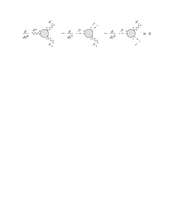
Figure 2: Graphical representation of Eq. (19) at any perturbative order.

Let’s now focus our attention on the A-B model of [6] where we have an anomalous generator $Y_{B}$. This model describes quite well many of the properties of the abelian sector of the general model discussed in [7] with a single anomalous $U(1)$. It is an ordinary gauge theory of the form $U(1)_{A}\times U(1)_{B}$ with $B$ made massive at tree level by the Stückelberg term

$$\mathcal{L}_{St}=\frac{1}{2}(\partial_{\mu}b+M_{1}B_{\mu})^{2}.$$ (20)

This term introduces a mixing $M_{1}B_{\mu}\partial^{\mu}b$ which signals the presence of a broken phase in the theory. Introducing the gauge fixing lagrangean

$$\mathcal{L}_{gf}=-\frac{1}{2\xi_{B}}(\mathcal{F}^{S}_{B}[B_{\mu}])^{2},$$ (21)

$$\mathcal{F}^{S}_{B}[B_{\mu}]\equiv\partial_{\mu}B^{\mu}-\xi_{B}M_{1}b,$$ (22)

we obtain the partial contributions (mass term plus gauge fixing term) to the total action

$$\mathcal{L}_{St}+\mathcal{L}_{gf}=\frac{1}{2}\biggl{[}(\partial_{\mu}b)^{2}+M_{1}^{2}B_{\mu}B^{\mu}-(\partial_{\mu}B^{\mu})^{2}-\xi_{B}M_{1}^{2}b^{2}\biggr{]}$$ (23)

and the corresponding Faddeev-Popov lagrangean

$$\mathcal{L}_{FP}=\bar{c}_{B}\,\frac{\delta\mathcal{F}_{B}}{\delta\theta_{B}}\,c_{B}=\bar{c}_{B}\,\biggl{[}\partial_{\mu}\frac{\delta B^{\mu}}{\delta\theta_{B}}-\xi_{B}M_{1}\,\frac{\delta b}{\delta\theta_{B}}\,\biggr{]}c_{B},$$ (24)

with $c_{B}$ and $\bar{c}_{B}$ are the anticommuting ghost/antighosts fields. It can be written as

$$\mathcal{L}_{FP}=\bar{c}_{B}\,(\square+\xi_{B}M_{1}^{2})\,c_{B},$$ (25)

having used the shift of the axion under a gauge transformation

$$\delta b=-M_{1}\theta.$$ (26)

In the following we will choose $\xi_{B}=1$. The anomalous sector is described by

$$\mathcal{S}_{an} = \mathcal{S}_{1}+\mathcal{S}_{3}$$

$$\mathcal{S}_{1} = \int dx\,dy\,dz\,\left(\frac{g_{B}\,g^{2}_{A}}{2!}\,T_{\bf AVV}^{\lambda\mu\nu}(x,y,z)B_{\lambda}(z)A_{\mu}(x)A_{\nu}(y)\right)$$

$$\mathcal{S}_{3} = \int dx\,dy\,dz\,\left(\frac{g^{3}_{B}}{3!}\,T_{\bf AAA}^{\lambda\mu\nu}(x,y,z)B_{\lambda}(z)B_{\mu}(x)B_{\nu}(y)\right),$$

where we have collected all the anomalous diagrams of the form (AVV and AAA) and whose gauge variations are

$$\frac{1}{2!}\delta_{B}\left[T_{\bf AVV}BAA\right] = \frac{i}{2!}a_{3}(\beta)\frac{1}{4}\left[F_{A}\wedge F_{A}\theta_{B}\right]$$

$$\frac{1}{3!}\delta_{B}\left[T_{\bf AAA}BBB\right] = \frac{i}{3!}\frac{a_{n}}{3}\frac{3}{4}\langle F_{B}\wedge F_{B}\theta_{B}\rangle,$$ (28)

having left open the choice over the parameterization of the loop momentum, denoted by the presence of the arbitrary parameter $\beta$ with

$$a_{3}(\beta)=-\frac{i}{4\pi^{2}}+\frac{i}{2\pi^{2}}\beta\qquad a_{3}\equiv\frac{a_{n}}{3}=-\frac{i}{6\pi^{2}},$$ (29)

while

$$\frac{1}{2!}\delta_{A}\left[T_{\bf AVV}BAA\right]=\frac{i}{2!}a_{1}(\beta)\frac{2}{4}\left[F_{B}\wedge F_{A}\theta_{A}\right].$$ (30)

We have the following equations for the anomalous variations

$$\delta_{B}\mathcal{L}_{an} = \frac{ig_{B}g^{\,2}_{A}}{2!}\,a_{3}(\beta)\frac{1}{4}F_{A}\wedge F_{A}\theta_{B}+\frac{ig^{\,3}_{B}}{3!}\,\frac{a_{n}}{3}\frac{3}{4}F_{B}\wedge F_{B}\theta_{B}$$

$$\delta_{A}\mathcal{L}_{an} = \frac{ig_{B}g^{\,2}_{A}}{2!}\,a_{1}(\beta)\frac{2}{4}F_{B}\wedge F_{A}\theta_{A},$$ (31)

while $\mathcal{L}_{b,c}$, the axionic contributions (Wess-Zumino terms) needed to restore the gauge symmetry violated at 1-loop level, are given by

$$\mathcal{L}_{b}=\frac{C_{AA}}{M}b\,F_{A}\wedge F_{A}+\frac{C_{BB}}{M}b\,F_{B}\wedge F_{B}.$$ (32)

The gauge invariance on $A$ requires that $\beta=-1/2\equiv\beta_{0}$ and is equivalent to a vector current conservation (CVC) condition. By imposing gauge invariance under B gauge transformations, on the other hand, we obtain

$$\delta_{B}\left(\mathcal{L}_{b}+\mathcal{L}_{an}\right)=0$$ (33)

which implies that

$$C_{AA}=\frac{i\,g_{B}g^{\,2}_{A}}{2!}\frac{1}{4}\,a_{3}(\beta_{0})\,\frac{M}{M_{1}},\qquad C_{BB}=\frac{ig^{\,3}_{B}}{3!}\frac{1}{4}\,a_{n}\,\frac{M}{M_{1}}.$$ (34)

This procedure, as we are going to show, is equivalent to the imposition of the STI on the corresponding anomalous vertices of the effective action. In fact the counterterms $C_{AA}$ and $C_{BB}$ can be determined formally from a BRST analysis.

In fact, the BRST variations of the model are defined as

$$\delta_{BRST}\,B_{\mu} = \omega\partial_{\mu}c_{B}$$

$$\delta_{BRST}\,b = -\omega M_{1}c_{B}$$

$$\delta_{BRST}\,A_{\mu} = \omega\,\partial_{\mu}c_{A}$$

$$\delta_{BRST}\,c_{B} = 0$$

$$\delta_{BRST}\,\bar{c}_{B} = \frac{\omega}{\xi_{B}}\mathcal{F}^{S}_{B}=\frac{\omega}{\xi_{B}}(\partial_{\mu}B^{\mu}-\xi_{B}M_{1}b).$$

To derive constraints on the 3-linear interactions involving 2 abelian (vector-like) and one vector-axial vector gauge field, that we will encounter in our analysis below, we require the BRST invariance of a specific correlator such as

$$\delta_{BRST}\,\langle 0|T\,\bar{c}_{B}(z)A_{\mu}(x)A_{\nu}(y)|0\rangle=0,$$ (36)

(Fig. 3 shows the difference between the non-amputated and the amputated correlators) and applying the BRST operator we obtain

$$\frac{\omega}{\xi_{B}}\,\langle 0|T\,[\partial_{\lambda}B^{\lambda}(z)-\xi_{B}M_{1}b(z)]A_{\mu}(x)A_{\nu}(y)|0\rangle + \langle 0|T\,\bar{c}_{B}(z)\omega\partial_{\mu}c_{A}(x)A_{\nu}(y)|0\rangle$$ (37)

$$+ \langle 0|T\,\bar{c}_{B}(z)A_{\mu}(x)\omega\partial_{\nu}c_{A}(y)|0\rangle=0,$$

with the last two terms being trivially zero. Choosing $\xi_{B}=1$ we obtain the STI (see Fig. 4) involving only the WZ term and the anomalous triangle diagram $BAA$. This reads

$$\frac{\partial}{\partial z^{\lambda}}\langle 0|T\,B^{\lambda}(z)A_{\mu}(x)A_{\nu}(y)|0\rangle-M_{1}\langle 0|T\,b(z)A_{\mu}(x)A_{\nu}(y)|0\rangle=0.$$ (38)

Figure 3: Relation between a correlator with non amputated external lines (left) used in a STI and an amputated one (right) used in the effective action for a triangle vertex and for a CS term.

Figure 4: Representation in terms of Feynman diagrams in momentum space of the Slavnov-Taylor identity obtained in the Stückelberg phase for the anomalous triangle $BAA$. Here we deal with correlators with non-amputated external lines. A CS term has been absorbed to ensure the conserved vector current (CVC) conditions on the A lines.

A similar STI holds for the BBB vertex and its counterterm

$$\frac{\partial}{\partial z^{\lambda}}\langle 0|T\,B^{\lambda}(z)B_{\mu}(x)B_{\nu}(y)|0\rangle-M_{1}\langle 0|T\,b(z)B_{\mu}(x)B_{\nu}(y)|0\rangle=0.$$ (39)

These two equations can be rendered explicit. For instance, to extract from (38) the corresponding expression in momentum space and the constraint on $C_{AA}$, we work at the lowest order in the perturbative expansion obtaining

$$\frac{1}{2!}\frac{\partial}{\partial z^{\lambda}}\langle 0|T\,B^{\lambda}(z)A_{\mu}(x)A_{\nu}(y)\left[J_{5}B\right]\left[JA\right]^{2}|0\rangle-M_{1}\langle 0|T\,b(z)A_{\mu}(x)A_{\nu}(y)\left[bF_{A}\wedge F_{A}\right]|0\rangle=0,$$

where we have introduced the notation $\left[\,\,\right]$ to denote the spacetime integration of the vector ($J$) and axial current ($J_{5}$) to their corresponding gauge fields

$$J\,A = -g_{A}\bar{\psi}\gamma^{\mu}\psi A_{\mu},$$ (41)

$$J_{5}\,B = -g_{B}\bar{\psi}\gamma^{\mu}\gamma^{5}\psi B_{\mu}$$ (42)

$$\tilde{J}_{5}\,G_{B} = 2ig_{B}\frac{m_{f}}{M_{B}}\bar{\psi}\gamma^{5}\psi G_{B}\,,$$ (43)

where $M_{B}$ is the mass of the $B$ gauge boson in the Higgs-Stückelberg phase that we will analyze in the next sections.

In momentum space the STI represented in Fig. 4 becomes $(\xi_{B}=1)$

$$\frac{1}{2!}\,2\,\left[ik^{\lambda^{\prime}}\right]\,\left[-\frac{ig_{\lambda\lambda^{\prime}}}{k^{2}-M_{1}^{2}}\right]\,\left[-\frac{ig_{\mu\mu^{\prime}}}{k_{1}^{2}}\right]\,\left[-\frac{ig_{\nu\nu^{\prime}}}{k_{2}^{2}}\right]\,\left[-g_{B}g_{A}^{2}\right]\,\Delta^{\lambda\mu\nu}(k_{1},k_{2})$$ (44)

$$- 2\,M_{1}\left[\frac{i}{k^{2}-M_{1}^{2}}\right]\,\left[-\frac{ig_{\mu\mu^{\prime}}}{k_{1}^{2}}\right]\,\left[-\frac{ig_{\nu\nu^{\prime}}}{k_{2}^{2}}\right]\,V^{\mu\nu}_{A}(k_{1},k_{2})=0,$$

where the factor $\frac{1}{2!}$ comes from the presence in the effective action of a diagram with 2 identical external lines, in this case two $A$ gauge bosons, and the factor $2$, present in both terms, comes from the possible contractions with the external fields. Using in (44) the corresponding anomaly equation

$$k_{\lambda}\Delta^{\lambda\mu\nu}(k_{1},k_{2})=a_{3}(\beta_{0})\epsilon^{\mu\nu\alpha\beta}k_{1\alpha}k_{2\beta}$$ (45)

and the expression of the vertex $V^{\mu\nu}_{A}(k_{1},k_{2})$

$$V^{\mu\nu}_{A}(k_{1},k_{2})=\frac{4C_{AA}}{M}\epsilon^{\mu\nu\alpha\beta}k_{1\alpha}k_{2\beta}$$ (46)

we obtain

$$\left[\frac{i}{k^{2}-M_{1}^{2}}\right]\,\left[-\frac{ig_{\mu\mu^{\prime}}}{k_{1}^{2}}\right]\,\left[-\frac{ig_{\nu\nu^{\prime}}}{k_{2}^{2}}\right]\,\biggl{[}i\,g_{B}g_{A}^{2}a_{3}(\beta_{0})\epsilon^{\mu\nu\alpha\beta}k_{1\alpha}k_{2\beta}-2\,M_{1}\frac{4C_{AA}}{M}\epsilon^{\mu\nu\alpha\beta}k_{1\alpha}k_{2\beta}\biggr{]}=0,$$

(47)

from which we get

$$i\,g_{B}g_{A}^{2}a_{3}(\beta_{0})=2\,M_{1}\frac{4C_{AA}}{M}\qquad\Rightarrow\qquad C_{AA}=\frac{i\,g_{B}g^{\,2}_{A}}{2}\frac{1}{4}\,a_{3}(\beta_{0})\,\frac{M}{M_{1}}.$$ (48)

This condition determines $C_{AA}$ at the same value as before in (36), using the constraints of gauge invariance, having brought the anomaly on the B vertex $(\beta_{0}=-1/2)$.

In the case of the second STI given in (39), expanding this equation at the lowest relevant order we get

$$\frac{1}{3!}\frac{\partial}{\partial z^{\lambda}}\langle 0|T\,B^{\lambda}(z)B_{\mu}(x)B_{\nu}(y)\left[J_{5}B\right]^{3}|0\rangle-M_{1}\langle 0|T\,b(z)B_{\mu}(x)B_{\nu}(y)\left[bF_{B}\wedge F_{B}\right]|0\rangle=0.$$ (49)

Also in this case, setting $\xi_{B}=1$, we re-express (49) as

$$\frac{1}{3!}\,3!\,\left[ik^{\lambda^{\prime}}\right]\,\left[-\frac{ig_{\lambda\lambda^{\prime}}}{k^{2}-M_{1}^{2}}\right]\,\left[-\frac{ig_{\mu\mu^{\prime}}}{k_{1}^{2}-M_{1}^{2}}\right]\,\left[-\frac{ig_{\nu\nu^{\prime}}}{k_{2}^{2}-M_{1}^{2}}\right]\,\left[-g_{B}^{3}\right]\,\Delta^{\lambda\mu\nu}(k_{1},k_{2})$$ (50)

$$- 2\,M_{1}\left[\frac{i}{k^{2}-M_{1}^{2}}\right]\,\left[-\frac{ig_{\mu\mu^{\prime}}}{k_{1}^{2}-M_{1}^{2}}\right]\,\left[-\frac{ig_{\nu\nu^{\prime}}}{k_{2}^{2}-M_{1}^{2}}\right]\,V^{\mu\nu}_{B}(k_{1},k_{2})=0,$$

where, similarly to $BAA$, the factor $\frac{1}{3!}$ comes from the 3 identical gauge B bosons on the external lines, the coefficient $3!$ in the first term counts all the contractions between the vertex $\Delta^{\lambda\mu\nu}$ and the propagators of the $B$ gauge bosons, while the coefficient $2$ comes from the contractions of $V^{\mu\nu}_{B}$ with the external lines. From Eq. (50) we get

$$\left[\frac{i}{k^{2}-M_{1}^{2}}\right]\,\left[-\frac{ig_{\mu\mu^{\prime}}}{k_{1}^{2}-M_{1}^{2}}\right]\,\left[-\frac{ig_{\nu\nu^{\prime}}}{k_{2}^{2}-M_{1}^{2}}\right]\,\biggl{[}ig_{B}^{3}\,k_{\lambda}\Delta^{\lambda\mu\nu}(k_{1},k_{2})-2\,M_{1}V^{\mu\nu}_{B}(k_{1},k_{2})\biggr{]}=0\,,$$ (51)

as depicted in Fig. 5.

Figure 5: Diagrammatic representation of (51) in the Stückelberg phase, determining the counterterm $C_{BB}$.

The anomaly equation for $BBB$ distributes the total anomaly $a_{n}$ equally among the three $B$ vertices, therefore

$$k_{\lambda}\Delta^{\lambda\mu\nu}(k_{1},k_{2})=\frac{a_{n}}{3}\epsilon^{\mu\nu\alpha\beta}k_{1\alpha}k_{2\beta},$$ (52)

and for the $V^{\mu\nu}_{B}(k_{1},k_{2})$ vertex we have

$$V^{\mu\nu}_{B}(k_{1},k_{2})=\frac{4C_{BB}}{M}\epsilon^{\mu\nu\alpha\beta}k_{1\alpha}k_{2\beta}.$$ (53)

Inserting (52), (53) into (51) we obtain

$$i\,g_{B}^{3}\,\frac{a_{n}}{3}=2\,M_{1}\,\frac{4C_{BB}}{M}\qquad\Rightarrow\qquad C_{BB}=\frac{i\,g^{3}_{B}}{2}\frac{1}{4}\,\frac{a_{n}}{3}\,\frac{M}{M_{1}},$$ (54)

in agreement with (36). Therefore we have shown that if we gauge-fix the effective lagrangean in the Sẗuckelberg phase to remove the b-B mixing and fix the CS counterterms so that the anomalous variations of the trilinear vertices are absent, we are actually imposing generalized Ward identities or STI’s on the effective action. On this gauge-fixed axion the b-B mixing is completely absent also off-shell and the structure of the trilinear vertices is rather simple. We need to check that these STI’s are compatible with those obtained after electroweak symmetry breaking, so that the mixing is absent off-shell also in the physical basis.

2.1 The Higgs-Stückelberg phase (HS)

Now consider the same effective action of the previous model after electroweak symmetry breaking. If we interpret the gauge-fixed action derived above as a completely determined theory where the counterterms have been found by the procedure that we have just illustrated, once we expand the fields around the Higgs vacuum we encounter a new mixing of the goldstones with the gauge fields. Due to Higgs-axion mixing [6] the goldstones of this theory are extracted by a suitable rotation that allows to separate physical from unphysical degrees of freedom. In fact the Stückelberg is decomposed into a physical axi-Higgs and a genuine goldstone. It is then natural to ask whether we could have just worked out the lagrangean directly in this phase by keeping the coefficients in front of the counterterms of the theory free, and had them fixed by imposing directly generalized WI’s in this phase, bypassing completely the first construction. As we are now going to show in this model the counterterms are determined consistently also in this case at the same values given before.

Let’s see how this happens. In this phase the mixing that needs to be eliminated is of the form $B^{\mu}\partial_{\mu}G_{B}$, where $G_{B}$ is the goldstone of the HS phase. In this case we use the gauge-fixing lagrangean

$$\mathcal{L}_{gf}=-\frac{1}{2\xi_{B}}(\mathcal{F}^{H}_{B})^{2}=-\frac{1}{2\xi_{B}}\left(\partial_{\mu}B^{\mu}-\xi_{B}M_{B}G_{B}\right),$$ (55)

and the BRST transformation of the antighost field $\bar{c}_{B}$ is given by

$$\delta_{BRST}\,\bar{c}_{B}=\frac{\omega}{\xi_{B}}\mathcal{F}^{H}_{B}=\frac{\omega}{\xi_{B}}\left(\partial_{\mu}B^{\mu}-\xi_{B}M_{B}G_{B}\right).$$ (56)

Also in this case we use the 3-point function in Eq. (36) and $\xi_{B}=1$ to obtain the STI

$$\frac{\partial}{\partial z^{\lambda}}\langle 0|T\,B^{\lambda}(z)A_{\mu}(x)A_{\nu}(y)|0\rangle-M_{B}\langle 0|T\,G_{B}(z)A_{\mu}(x)A_{\nu}(y)|0\rangle=0.$$ (57)

Figure 6: Diagrammatic representation of Eq. (58) in the HS phase, determining the counterterm $C_{AA}$. A CS term has been absorbed by the CVC conditions on the $A$ gauge bosons.

To get insight into this equation we expand perturbatively (57) and obtain

$$\frac{1}{2!}\,\frac{\partial}{\partial z^{\lambda}}\,\langle 0|T\,B^{\lambda}(z)A_{\mu}(x)A_{\nu}(y)\left[J_{5}B\right]\left[JA\right]^{2}|0\rangle$$

$$-\,M_{B}\,\langle 0|T\,G_{B}(z)A_{\mu}(x)A_{\nu}(y)\left[G_{B}F_{A}\wedge F_{A}\right]|0\rangle$$

$$-\,M_{B}\,\langle 0|T\,G_{B}(z)A_{\mu}(x)A_{\nu}(y)\left[\tilde{J}_{5}G_{B}\right]\left[JA\right]^{2}|0\rangle=0,$$ (58)

where the first term is the usual triangle diagram with the $BAA$ gauge bosons on the external lines, the second is a WZ vertex with $G_{B}$ on the exernal line and the third term, which is absent in the Stückelberg phase, is a triangle diagram involving the $G_{B}$ gauge boson that couples to the fermions by a Yukawa coupling (see Fig. 6). In the Stückelberg phase there is no analogue of this third contribution in the cancellation of the anomalies for this vertex, since $b$ does not couple to the fermions.

Notice that the STI now contains a vertex derived from the $bF_{A}\wedge F_{A}$ counterterm, but projected on the interaction $G_{B}F_{A}\wedge F_{A}$ via the factor $M_{1}/M_{B}$. This factor is generated by the rotation matrix that allows the change of variables $(\phi_{2},b)\to(\chi_{B},G_{B})$ and is given by

$$U=\left(\begin{array}[]{ll}-\cos\theta_{B}&\sin\theta_{B}\\ \sin\theta_{B}&\cos\theta_{B}\end{array}\right)$$ (59)

with $\theta_{B}={\arccos}({M_{1}/M_{B}})={\arcsin}(q_{B}g_{B}v/M_{B})$. We recall [6] that the axion $b$ can be expressed as a linear combination of the rotated fields $\chi$ and $G_{B}$ of the form

$$b=\alpha_{1}\chi_{B}+\alpha_{2}G_{B}=\frac{q_{B}g_{B}v}{M_{B}}\chi_{B}+\frac{M_{1}}{M_{B}}G_{B},$$ (60)

where $\chi$ is the physical axion and $G_{B}$ the Goldstone boson; we also recall that the gauge field $B_{\mu}$ gets its mass $M_{B}$ through the combined Higgs-Stückelberg mechanism

$$M_{B}=\sqrt{M_{1}^{2}+(q_{B}g_{B}v)^{2}}.$$ (61)

Now we express the STI given in (58) choosing $\xi_{B}=1$

$$\frac{1}{2!}\,2\,\left[ik^{\lambda^{\prime}}\right]\,\left[-\frac{ig_{\lambda\lambda^{\prime}}}{k^{2}-M_{B}^{2}}\right]\,\left[-\frac{ig_{\mu\mu^{\prime}}}{k_{1}^{2}}\right]\,\left[-\frac{ig_{\nu\nu^{\prime}}}{k_{2}^{2}}\right]\,\left[-g_{B}g_{A}^{2}\right]\,\Delta^{\lambda\mu\nu}(m_{f},k_{1},k_{2})$$

$$- \,M_{B}\left[\frac{i}{k^{2}-M_{B}^{2}}\right]\,\left[-\frac{ig_{\mu\mu^{\prime}}}{k_{1}^{2}}\right]\,\left[-\frac{ig_{\nu\nu^{\prime}}}{k_{2}^{2}}\right]\,\biggl{\{}2\,\frac{M_{1}}{M_{B}}\,V^{\mu\nu}_{A}(k_{1},k_{2})$$

$$\hskip 99.58464pt+\frac{1}{2!}\,2\,i\,g_{B}g_{A}^{2}\,\left(2i\,\frac{m_{f}}{M_{B}}\right)\,\Delta^{\mu\nu}_{G_{B}AA}(m_{f},k_{1},k_{2})\biggr{\}}=0,$$

where the $\left[G_{B}F_{A}\wedge F_{A}\right]$ interaction has been obtained from the $\left[bF_{A}\wedge F_{A}\right]$ vertex by projecting the $b$ field on the field $G_{B}$, and the coefficient $2im_{f}/M_{B}$ comes from the coupling of $G_{B}$ with the massive fermions [6]. The remaining coefficient $M_{1}/M_{B}$ rotates the $V^{\mu\nu}_{A}(k_{1},k_{2})$ vertex as in Eq. (LABEL:BAA_STprime).

Replacing in (LABEL:BAA_STprime) the WI obtained for a massive AVV vertex

$$k_{\lambda}\Delta^{\lambda\mu\nu}(\beta,m_{f},k_{1},k_{2}) = a_{3}(\beta)\varepsilon^{\mu\nu\alpha\beta}k_{1}^{\alpha}k_{2}^{\beta}+2m_{f}\Delta^{\mu\nu}(m_{f},k_{1},k_{2}),$$ (63)

where

$$\Delta^{\mu\nu}(m_{f},k_{1},k_{2})=m_{f}\varepsilon^{\alpha\beta\mu\nu}k_{1,\alpha}k_{2,\beta}\left(\frac{1}{2\pi^{2}}\right)I(m_{f})$$

$$I(m_{f})\equiv-\int_{0}^{1}\int_{0}^{1-x}dxdy\frac{1}{m_{f}^{2}+(x-1)xk_{1}^{2}+(y-1)yk_{2}^{2}-2xyk_{1}\cdot k_{2}},$$ (64)

and the expression for the $V^{\mu\nu}_{A}(k_{1},k_{2})$ vertex

$$V^{\mu\nu}_{A}(k_{1},k_{2})=\frac{4C_{AA}}{M}\epsilon^{\mu\nu\alpha\beta}k_{1\alpha}k_{2\beta},$$ (65)

we get

$$\left[\frac{ig_{\lambda\lambda^{\prime}}}{k^{2}-M_{B}^{2}}\right]\,\left[\frac{ig_{\mu\mu^{\prime}}}{k_{1}^{2}}\right]\,\left[\frac{ig_{\nu\nu^{\prime}}}{k_{2}^{2}}\right]\,\biggl{\{}i\,g_{B}g_{A}^{2}\,a_{3}(\beta_{0})\,\epsilon^{\mu\nu\alpha\beta}k_{1\alpha}k_{2\beta}$$

$$+2\,i\,g_{B}g_{A}^{2}\,m_{f}\,\Delta^{\mu\nu}(m_{f},k_{1},k_{2})-2\,M_{B}\,\frac{4C_{AA}}{M}\epsilon^{\mu\nu\alpha\beta}k_{1\alpha}k_{2\beta}$$

$$-2\,ig_{B}g_{A}^{2}\,M_{B}\,\frac{m_{f}}{M_{B}}\,\Delta^{\mu\nu}_{G_{B}AA}(m_{f},k_{1},k_{2})\biggr{\}}=0.$$ (66)

Since $\Delta^{\mu\nu}_{G_{B}AA}=\Delta^{\mu\nu}$, Eq.(66) yields the same condition obtained by fixing $C_{AA}$ in the Stückelberg phase, that is

$$i\,g_{B}g_{A}^{2}a_{3}(\beta_{0})=2\,M_{1}\frac{4C_{AA}}{M}\qquad\Rightarrow\qquad C_{AA}=\frac{i\,g_{B}g^{\,2}_{A}}{2}\frac{1}{4}\,a_{3}(\beta_{0})\,\frac{M}{M_{1}}.$$ (67)

A similar STI can be derived for the $BBB$ vertex in this phase, obtaining

$$\frac{\partial}{\partial z^{\lambda}}\langle 0|T\,B^{\lambda}(z)B_{\mu}(x)B_{\nu}(y)|0\rangle-M_{B}\langle 0|T\,G_{B}(z)B_{\mu}(x)B_{\nu}(y)|0\rangle=0.$$ (68)

Expanding perturbatively (68) we obtain

$$\frac{1}{3!}\,\frac{\partial}{\partial z^{\lambda}}\,\langle 0|T\,B^{\lambda}(z)B_{\mu}(x)B_{\nu}(y)\left[J_{5}B\right]^{3}|0\rangle$$

$$-\,M_{B}\,\langle 0|T\,G_{B}(z)B_{\mu}(x)B_{\nu}(y)\left[G_{B}F_{B}\wedge F_{B}\right]|0\rangle$$

$$-\,M_{B}\,\langle 0|T\,G_{B}(z)B_{\mu}(x)B_{\nu}(y)\left[\tilde{J}_{5}G_{B}\right]\left[J_{5}B\right]^{2}|0\rangle=0,$$ (69)

that gives

$$\frac{1}{3!}\,3!\,\left[ik^{\lambda^{\prime}}\right]\left[-\frac{ig_{\lambda\lambda^{\prime}}}{k^{2}-M_{B}^{2}}\right]\left[-\frac{ig_{\mu\mu^{\prime}}}{k_{1}^{2}-M_{B}^{2}}\right]\left[-\frac{ig_{\nu\nu^{\prime}}}{k_{2}^{2}-M_{B}^{2}}\right]\left[-g_{B}^{3}\right]\Delta^{\lambda\mu\nu}(m_{f},k_{1},k_{2})$$

$$-\,M_{B}\left[\frac{i}{k^{2}-M_{B}^{2}}\right]\,\left[-\frac{ig_{\mu\mu^{\prime}}}{k_{1}^{2}-M_{B}^{2}}\right]\,\left[-\frac{ig_{\nu\nu^{\prime}}}{k_{2}^{2}-M_{B}^{2}}\right]\,\biggl{\{}2\,\frac{M_{1}}{M_{B}}\,V^{\mu\nu}_{B}(k_{1},k_{2})$$

$$+\frac{1}{2!}\,2\,i\,g_{B}^{3}\,\left(2i\,\frac{m_{f}}{M_{B}}\right)\,\Delta^{\mu\nu}_{G_{B}BB}(m_{f},k_{1},k_{2})\biggr{\}}=0,$$

(70)

where we have defined

$$\Delta^{\mu\nu}_{G_{B}BB}=\int\frac{d^{4}q}{(2\pi)^{4}}\frac{Tr\left[\gamma^{5}(q\hskip-6.0pt/\hskip 6.0pt-k\hskip-6.0pt/\hskip 6.0pt+m_{f})\gamma^{\nu}\gamma^{5}(q\hskip-6.0pt/\hskip 6.0pt-k_{1}\hskip-6.0pt/\hskip 6.0pt+m_{f})\gamma^{\mu}\gamma^{5}(q\hskip-6.0pt/\hskip 6.0pt+m_{f})\right]}{\left[q^{2}-m^{2}_{f}\right]\left[(q-k)^{2}-m^{2}_{f}\right]\left[(q-k_{1})^{2}-m^{2}_{f}\right]}$$

$$\hskip 56.9055pt+\left\{\mu\leftrightarrow\nu,k_{1}\leftrightarrow k_{2}\right\}\,.$$ (71)

Since this contribution is finite, it gives

$$\Delta^{\mu\nu}_{G_{B}BB}=2\int\frac{d^{4}q}{(2\pi)^{4}}\int_{0}^{1}\int_{0}^{1-x}dxdy\frac{2m4i\varepsilon^{\mu\nu\alpha\beta}k_{1,\alpha}k_{2,\beta}}{\left[q^{2}-k_{2}^{2}(y-1)y-k_{1}^{2}(x-1)x+2xy-m_{f}^{2}\right]^{3}}$$ (72)

and we obtain again

$$\Delta^{\mu\nu}_{G_{B}BB}=\Delta^{\mu\nu}=\varepsilon^{\alpha\beta\mu\nu}k_{1,\alpha}k_{2,\beta}m_{f}\left(\frac{1}{2\pi^{2}}\right)I(m_{f})\,,$$ (73)

Using the anomaly equations in the chirally broken phase

$$k_{\lambda}\Delta_{3}^{\lambda\mu\nu}(k_{1},k_{2}) = \frac{a_{n}}{3}\varepsilon^{\mu\nu\alpha\beta}k_{1}^{\alpha}k_{2}^{\beta}+2m_{f}\Delta^{\mu\nu}$$ (74)

and the expression of the vertex

$$V^{\mu\nu}_{B}(k_{1},k_{2})=\frac{4C_{BB}}{M}\epsilon^{\mu\nu\alpha\beta}k_{1\alpha}k_{2\beta},$$ (75)

we obtain

$$C_{BB}=\frac{i\,g^{3}_{B}}{2}\frac{1}{4}\,\frac{a_{n}}{3}\,\frac{M}{M_{1}}.$$ (76)

Expanding to the lowest nontrivial order this identity we obtain

$$i\left(\frac{a_{n}}{3}\epsilon^{\mu\nu\alpha\beta}k_{1\alpha}k_{2\beta}+2m_{f}\Delta^{\mu\nu}\right)-2M_{B}\left(\frac{4}{M}C_{BB}\frac{M_{1}}{M_{B}}\right)\epsilon^{\mu\nu\alpha\beta}k_{1\alpha}k_{2\beta}-M_{B}\left(2i\frac{m_{f}}{M_{B}}\right)\Delta^{\mu\nu}_{G_{B}BB}=0,$$ (77)

which can be easily solved for $C_{BB}$, thereby determining $C_{BB}$ exactly at the same value inferred from the Stückelberg phase, as discussed above.

2.2 Slavnov-Taylor Identities and BRST symmetry in the complete model

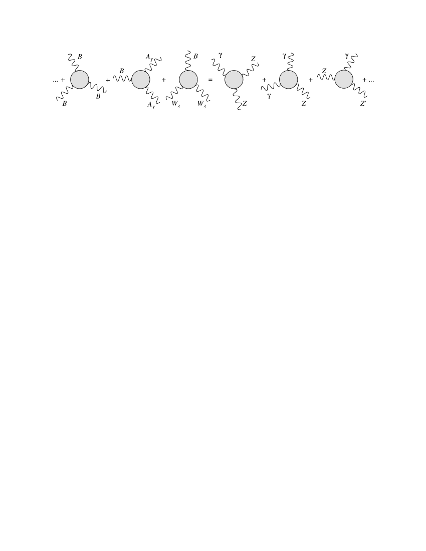
Figure 7: The anomalous effective action in the two basis in the $R_{\xi}$ gauge where we have eliminated the mixings on the external lines in both basis.

It is obvious, from the analysis presented above, that a similar treatment is possible also in the non-abelian case, though the explicit analysis is more complex. The objective of this investigation, however, is by now clear: we need to connect the anomalous effective action of the general model in the interaction basis and in the mass eigenstate basis keeping into account that both phases are broken phases. In Fig. 7 this point is shown pictorially. In both cases the bilinear mixings of the goldstones with the corresponding gauge fields, $Z\partial G_{Z},Z^{\prime}\partial G_{Z^{\prime}}$ have been removed and the counterterms in the eigenstate basis have been fixed as in [7], where we have just shown it for the A-B model. Equivalently, we can fix the counterterms in the HS phase by imposing the STI’s directly at this stage, thereby defining the anomalous effective action plus WZ terms completely. For this we need the BRST transformation of the fundamental fields. As usual, in the gauge sector these can be obtained by replacing the gauge parameter in their gauge variations with the corresponding ghost fields times a Grassmann parameter $\omega$. Denoting by $s$ the BRST operator, these are given by

$$sA^{\gamma}_{\mu}=\omega\,\partial_{\mu}c_{\gamma}+i\,O^{A}_{11}\,g_{2}\,\omega\left(c^{-}W^{+}_{\mu}-c^{+}W^{-}_{\mu}\right),$$ (78)

$$sZ_{\mu}=\omega\,\partial_{\mu}c_{Z}+i\,O^{A}_{21}\,g_{2}\,\omega\,\left(c^{-}W^{+}_{\mu}-c^{+}W^{-}_{\mu}\right),$$ (79)

$$sZ^{\prime}_{\mu}=\omega\,\partial_{\mu}c_{Z^{\prime}}+i\,O^{A}_{31}\,g_{2}\,\omega\left(c^{-}W^{+}_{\mu}-c^{+}W^{-}_{\mu}\right)$$ (80)

$$s\,W^{{\tt+}}_{\mu} = \omega\,\partial_{\mu}c^{{\tt+}}-ig_{2}W^{{\tt+}}_{\mu}\,\omega\left(O^{A}_{11}c_{\gamma}+O^{A}_{21}c_{Z}+O^{A}_{31}c_{Z^{\prime}}\right)$$ (81)

$$+ ig_{2}\,\left(O^{A}_{11}A_{\gamma\mu}+O^{A}_{21}Z_{\mu}+O^{A}_{31}Z^{\prime}_{\mu}\right)\omega c^{{\tt+}},$$

$$sW^{{\tt-}}_{\mu} = \omega\partial_{\mu}c^{{\tt-}}+ig_{2}W^{{\tt-}}_{\mu}\omega\,\left(O^{A}_{11}c_{\gamma}+O^{A}_{21}c_{Z}+O^{A}_{31}c_{Z^{\prime}}\right)$$ (82)

$$- ig_{2}\left(O^{A}_{11}A_{\gamma\mu}+O^{A}_{21}Z_{\mu}+O^{A}_{31}Z^{\prime}_{\mu}\right)\omega c^{{\tt-}},$$

where the $O^{A}_{ij}$ are matrix elements defined exactly as in Eq. (103) below. To determine the transformations rules for the ghost/antighost fields we recall that the gauge-fixing lagrangeans in the $R_{\xi}$ gauge are given by

$$\mathcal{L}_{gf}^{Z} = -\frac{1}{2\xi_{Z}}\mathcal{F}[Z,G^{Z}]^{2}=-\frac{1}{2\xi_{Z}}(\partial_{\mu}Z^{\mu}-\xi_{Z}M_{Z}G^{Z})^{2},$$ (83)

$$\mathcal{L}_{gf}^{Z^{\prime}} = -\frac{1}{2\xi_{Z^{\prime}}}\mathcal{F}[Z^{\prime},G^{Z^{\prime}}]^{2}=-\frac{1}{2\xi_{Z^{\prime}}}(\partial_{\mu}Z^{\prime\mu}-\xi_{Z^{\prime}}M_{Z^{\prime}}G^{Z^{\prime}})^{2},$$ (84)

$$\mathcal{L}_{gf}^{A_{\gamma}} = -\frac{1}{2\xi_{A}}\mathcal{F}[A_{\gamma}]^{2}=-\frac{1}{2\xi_{A}}(\partial_{\mu}A_{\gamma}^{\mu})^{2},$$ (85)

$$\mathcal{L}_{gf}^{W} = -\frac{1}{\xi_{W}}\mathcal{F}[W^{+},G^{+}]\mathcal{F}[W^{-},G^{-}]=$$ (86)

$$= -\frac{1}{\xi_{W}}(\partial_{\mu}W^{+\mu}+i\xi_{W}M_{W}G^{+})(\partial_{\mu}W^{-\mu}-i\xi_{W}M_{W}G^{-}),$$

where $G^{Z}$, $G^{Z^{\prime}}$, $G^{+}$ and $G^{-}$ are the goldstones of $Z$, $Z^{\prime}$, $W^{+}$ and $W^{-}$ respectively.

In particular, the FP (ghost) part of the lagrangean is canonically given by

$$\mathcal{L}_{FP}=-\bar{c}^{a}\frac{\delta\mathcal{F}^{a}[Z,z]}{\delta\theta^{b}}c^{b},$$ (87)

where the sum over $a$ and $b$ runs over the fields $Z$, $Z^{\prime}$, $A_{\gamma}$, $W^{+}$ e $W^{-}$ and is explicitly given in the appendix. For the BRST variations of the antighosts we obtain

$$s\,\bar{c}_{a}=-\frac{i}{\xi_{a}}\,\omega\,\mathcal{F}^{a}\qquad\qquad a=Z,Z^{\prime},\gamma,+,-$$ (88)

and in particular

$$s\,\bar{c}_{Z} = -\frac{i}{\xi_{Z}}\,\omega\,\left(\partial_{\mu}Z^{\mu}-\xi_{Z}M_{Z}G^{Z}\right)$$ (89)

$$s\,\bar{c}_{Z^{\prime}} = -\frac{i}{\xi_{Z^{\prime}}}\,\omega\,\left(\partial_{\mu}Z^{\prime\mu}-\xi_{Z^{\prime}}M_{Z^{\prime}}G^{Z^{\prime}}\right)$$ (90)

$$s\,\bar{c}_{\gamma} = -\frac{i}{\xi_{\gamma}}\,\omega\,\left(\partial_{\mu}A_{\gamma}^{\mu}\right)$$ (91)

$$s\,\bar{c}_{+} = -\frac{i}{\xi_{W}}\,\omega\,\left(\partial_{\mu}W^{+\mu}+i\xi_{W}M_{W}G^{+}\right)$$ (92)

$$s\,\bar{c}_{-} = -\frac{i}{\xi_{W}}\,\omega\,\left(\partial_{\mu}W^{-\mu}-i\xi_{W}M_{W}G^{-}\right),$$ (93)

giving typically the STI

$$\frac{\partial}{\partial z^{\lambda}}\langle 0|T\,Z^{\lambda}(z)A_{\mu}(x)A_{\nu}(y)|0\rangle-M_{Z}\langle 0|T\,G_{Z}(z)A_{\mu}(x)A_{\nu}(y)|0\rangle=0,$$ (94)

and a similar one for the $Z^{\prime}$ gauge boson.

We pause for a moment to emphasize the difference between this STI and the corresponding one in the SM. In this latter case the structure of the STI is

$$k_{\rho}\,G^{\rho\nu\mu} = (k_{1}+k_{2})_{\rho}\,G^{\,\rho\nu\mu}$$ (95)

$$= \frac{e^{2}g}{\pi^{2}\cos\theta_{W}}\sum_{f}g^{f}_{A}Q^{2}_{f}\,\epsilon^{\,\nu\mu\alpha\beta}k_{1\alpha}k_{2\beta}\,\left[-m^{2}_{f}\int^{1}_{0}dx_{1}\int^{1-x_{1}}_{0}dx_{2}\,\frac{1}{\Delta}\right],$$

where $G^{\rho\nu\mu}$ is the gauge boson vertex, which is shown pictorially in Fig. 9 (diagrams a and c). Notice that the goldstone contribution is the factor in square brackets in the expression above, being the coupling of the Goldstone proportional to $m_{f}^{2}/M_{Z}$. In the chiral limit the STI of the $Z\gamma\gamma$ vertex of the Standard Model becomes an ordinary Ward identity, as in the photon case. In Fig. 9 the modification due to the presence of the WZ term is evident. In fact, expanding (94) in the anomalous case we have

$$k_{\rho}\,G^{\rho\nu\mu} = (k_{1}+k_{2})_{\rho}\,G^{\,\rho\nu\mu}$$ (96)

$$= \frac{e^{2}g}{\pi^{2}\cos\theta_{W}}\sum_{f}g^{f}_{A}Q^{2}_{f}\,\epsilon^{\,\nu\mu\alpha\beta}k_{1\alpha}k_{2\beta}\,\left[\frac{1}{2}-m^{2}_{f}\int^{1}_{0}dx_{1}\int^{1-x_{1}}_{0}dx_{2}\,\frac{1}{\Delta}\right],$$

where the first term in the square brackets is now the WZ contribution and the second the usual goldstone contribution, as in the SM case. Notice that the factor $\sum_{f}g^{f}_{A}Q^{2}_{f}$ is in fact proportional to the total chiral asymmetry of the $Z$ vertex, which is mass independent and appears as a factor in front of the WZ counterterm. In the chiral limit the anomalous STI is represented in Fig. 9.

Figure 8: The general STI for the $Z\gamma\gamma$ vertex in our anomalous model away from the chiral limit. The analogous STI for the SM case consists of only diagrams a) and c).

Figure 9: The STI for the $Z\gamma\gamma$ vertex for our anomalous model and in the chiral phase. The analogous STI in the SM consists of only diagram a).

At this point we are ready to proceed with a more general analysis of the trilinear gauge interactions to derive the expressions of all the anomalous vertices of a given theory in the mass eigenstate basis and away from the chiral limit. The reason for stressing this aspect has to do with the way the chiral symmetry breaking effects appear in the SM and in the anomalous models. In particular, we will start by extending the analysis presented in [7] for the derivation of the $Z\gamma\gamma$ vertex, which is here presented in far more detail. Compared to [7] we show some unobvious features of the derivation which are essential in order to formulate general rules for the computation of these vertices. We rotate the fields from the interaction eigenstate basis to the physical basis and the CS counterterms are partly absorbed and the anomaly is moved from the anomaly-free gauge boson vertices to the anomalous ones. This analysis is then extended to other trilinear vertices and we finally provide general rules to handle these types of interactions for a generic number of $U(1)$’s.

Before we come to the analysis of this vertex, we recall that the neutral current sector of the model is defined as [7]

$$-{\mathcal{L}}_{NC}=\overline{\psi}_{f}\gamma^{\mu}\mathcal{F}\psi_{f},$$ (97)

with

$$\mathcal{F}=g_{2}W^{3}_{\mu}T^{\,3}+g_{Y}YA^{Y}_{\mu}+g_{B}Y_{B}B_{\mu}$$ (98)

expressed in the interaction eigenstate basis. Equivalently it can be re-expressed as

$$\mathcal{F} = g_{Z}Q_{Z}Z_{\mu}+g_{Z^{\prime}}Q_{Z^{\prime}}Z^{\prime}_{\mu}+e\,QA^{\gamma}_{\mu},$$ (99)

where $Q=T^{3}+Y$. The physical fields $A^{\gamma},Z,Z^{\prime}$ and $W_{3},A^{Y},B$ are related by the rotation matrix $O^{A}$ to the interaction eigenstates

$$\pmatrix{A^{\gamma}\cr Z\cr{{Z^{\prime}}}}=O^{A}\,\pmatrix{W_{3}\cr A^{Y}\cr B}$$ (100)

or equivalently

$$W^{3}_{\mu} = O^{A}_{W_{3}\gamma}A^{\gamma}_{\mu}+O^{A}_{W_{3}Z}Z_{\mu}+O^{A}_{W_{3}Z^{\prime}}Z^{\prime}_{\mu}$$ (101)

$$A^{Y}_{\mu} = O^{A}_{Y\gamma}A^{\gamma}_{\mu}+O^{A}_{YZ}Z_{\mu}+O^{A}_{YZ^{\prime}}Z^{\prime}_{\mu}$$ (102)

$$B_{\mu} = O^{A}_{BZ}Z_{\mu}+O^{A}_{BZ^{\prime}}Z^{\prime}_{\mu}.$$ (103)

Substituting these transformations in the expression of the bosonic operator $\mathcal{F}$ and reading the coefficients of the fields $Z_{\mu},Z^{\prime}_{\mu}$ and $A^{\gamma}_{\mu}$ we obtain this set of relations for the coupling constants and the generators in the two basis, given here in a chiral form

$$g_{Z}Q_{Z}^{L} = g_{2}T^{3L}O^{A}_{W_{3}Z}+g_{Y}Y^{L}O^{A}_{YZ}+g_{B}Y_{B}^{L}O^{A}_{BZ}$$ (104)

$$g_{Z}Q_{Z}^{R} = g_{Y}Y^{R}O^{A}_{YZ}+g_{B}Y_{B}^{R}O^{A}_{BZ}$$ (105)

$$g_{Z^{\prime}}Q_{Z^{\prime}}^{L} = g_{2}T^{3L}O^{A}_{W_{3}Z^{\prime}}+g_{Y}Y^{L}O^{A}_{YZ^{\prime}}+g_{B}Y_{B}^{L}O^{A}_{BZ^{\prime}}$$ (106)

$$g_{Z^{\prime}}Q_{Z^{\prime}}^{R} = g_{Y}Y^{R}O^{A}_{YZ^{\prime}}+g_{B}Y_{B}^{R}O^{A}_{BZ^{\prime}}$$ (107)

$$eQ^{L} = g_{2}T^{3L}O^{A}_{W_{3}A}+g_{Y}Y^{L}O^{A}_{YA}=g_{Y}Y^{R}O^{A}_{YA}=eQ^{R}.$$ (108)

3 General analysis of the $Z\gamma\gamma$ vertex

Let’s now come to a brief analysis of this vertex, stressing on the general features of its derivation, which has not been detailed in [7]. In particular we highlight the general approach to follow in order to derive these vertices and apply it to the case when several anomalous $U(1)$’s are present. We will exploit the invariance of the anomalous part of the effective action under transformations of the external classical fields. This is illustrated in Fig. 7. More formally we can set

$$W_{anom}(B,W,A_{Y})=W_{anom}(Z,Z^{\prime},A_{\gamma}),$$ (109)

where we limit our analysis to the anomalous contributions.

In the chiral phase, the triangle diagrams projecting on this vertex are the following: $YYY$, $YW_{3}W_{3}$, $BYY$ and $BW_{3}W_{3}$. They are represented in Fig. 10, where we have added the corresponding counterterms.

Figure 10: All the triangle diagrams and the possible CS and WZ counterterms present in the model (chiral phase). Not all these diagrams project on $Z\rightarrow\gamma\gamma$ in the mass eigenstate basis.

The first two are SM-like and hence anomaly-free by charge assignment. The diagrams involving the $B$ gauge boson are typical of these models, are anomalous, and require suitable counterterms in order to cancel their anomalies. All the possible counterterms are shown in Fig. 10. The WZ terms of the form $bYY$ or $bW_{3}W_{3}$ will project both on a $G_{Z}\gamma\gamma$ and a $\chi\gamma\gamma$ interactions, the first one being relevant for the STI of the vertex. The main issue to be addressed is that of the distribution of the anomaly among the triangular vertices. These points have been discussed in [6] and [7] working in the chiral limit, when the fermion masses are removed from the diagrams.

Figure 11: The routing of the anomaly and the absorption of the CS term into the anomalous $B$ gauge boson. The anomaly is distributed among the vertices with the black dot.

The procedure can follow, equivalently, two directions: we can start from the $BYW_{3}$ basis and project onto the vertices $Z\gamma\gamma,ZZ\gamma$…, rotating the fields (not the charges) or, equivalently, start from the $Z,Z^{\prime}\gamma$ basis and rotate the charges (but not the fields) and the generators onto the interaction eigenstate basis $BYW_{3}$. We obtain two equivalent descriptions of the various vertices. In the interaction basis the CS terms are absorbed and the anomaly is moved from the $Y$ or $W$ vertices into the B vertex, where it is cancelled by the axion (see Fig. 11). This is the meaning of the STI’s shown above. Therefore it is clear that most of the CS terms do not appear explicitly if we use this approach. On the other hand, if we work in the mass eigenstate basis they can be kept explicit, but one has to be careful because in this case also the remaining vertices containing the generator of the electric charge $Q\sim Y+T_{3}$ have partial anomalies. The two approaches, as we are going to see, can be combined in a very economical way in some special cases, for instance for the $Z\gamma\gamma$ vertex, where one can attach all the anomaly to the Z gauge boson and add only the $G_{Z}\gamma\gamma$ counterterm. Similarly, for other interactions such as the $ZZ\gamma$ vertex, the total anomaly has to be equally distributed between the two $Z^{\prime}$s, since only the B generator carries an anomaly in the chiral limit, if we choose to absorb the CS terms. For other vertices such as $ZZZ^{\prime}$ etc, all the vertices contribute to the total anomaly and their partial contributions can be identified by decomposing the corresponding triangle in the $YBW_{3}$ basis with some CS terms left over.

4 The $\langle Z_{l}\gamma\gamma\rangle$ vertex

In this section we begin our technical discussion of the method. Since the most general case is encountered when at least 3 anomalous $U(1)$’s are present in the theory, we will consider for definiteness a model with three of them, say $B_{j}=\{B_{1},B_{2},B_{3}\}$. We can write the field transformation from interaction eigenstates basis to the mass eigenstates basis as

$$W_{3}=O^{A}_{W_{3}\gamma}A_{\gamma}+\sum_{l=0}^{3}O^{A}_{W_{3}Z_{l}}Z_{l}$$

$$Y=O^{A}_{Y\gamma}A_{\gamma}+\sum_{l=0}^{3}O^{A}_{YZ_{l}}Z_{l}$$

$$B_{j}=O^{A}_{B_{j}\gamma}A_{\gamma}+\sum_{l=0}^{3}O^{A}_{B_{j}Z_{l}}Z_{l},$$ (110)

with $j=1,2,3$, where for $l=0$ we have the $Z_{0}$ belonging to the SM and $Z_{1},Z_{2},Z_{3}$ are the anomalous ones. As in [7] we rotate the external field of the anomalous interactions from one base to the other, selecting the projections over the $Z_{l}\gamma\gamma$ vertex (the ellipsis indicate additional contributions that have no projection on the vertex that we consider)

$$\frac{1}{3!}Tr\left[Q_{Y}^{3}\right]\langle YYY\rangle=\frac{1}{3!}Tr\left[Q_{Y}^{3}\right]R^{YYY}_{Z_{l}\gamma\gamma}\langle Z_{l}\gamma\gamma\rangle+\dots$$

$$\frac{1}{2!}Tr\left[Q_{Y}T_{3}^{2}\right]\langle YWW\rangle=\frac{1}{2!}Tr\left[Q_{Y}T_{3}^{2}\right]R^{YWW}_{Z_{l}\gamma\gamma}\langle Z_{l}\gamma\gamma\rangle+\dots$$

$$\frac{1}{2!}Tr\left[Q_{B_{j}}Q_{Y}^{2}\right]\langle B_{j}YY\rangle=\frac{1}{2!}Tr\left[Q_{B_{j}}Q_{Y}^{2}\right]R^{B_{j}YY}_{Z_{l}\gamma\gamma}\langle Z_{l}\gamma\gamma\rangle+\dots$$

$$\frac{1}{2!}Tr\left[Q_{B_{j}}T_{3}^{2}\right]\langle B_{j}WW\rangle=\frac{1}{2!}Tr\left[Q_{B_{j}}T_{3}^{2}\right]R^{WWB_{j}}_{Z_{l}\gamma\gamma}\langle Z_{l}\gamma\gamma\rangle+\dots$$

where the rotation coefficients $R^{YYY}_{Z_{l}\gamma\gamma},R^{YWW}_{Z_{l}\gamma\gamma},R^{B_{i}YY}_{Z_{l}\gamma\gamma},R^{B_{i}WW}_{Z_{l}\gamma\gamma}$ containing several products of the elements of the rotation matrix $O^{A}$ are given by

$$R^{YYY}_{Z_{l}\gamma\gamma}=3\left[(O^{A})_{YZ_{l}}(O^{A})_{Y\gamma}^{2}\right]$$

$$R^{YWW}_{Z_{l}\gamma\gamma}=\left[2(O^{A})_{W_{3}\gamma}(O^{A})_{YZ_{l}}(O^{A})_{Y\gamma}+(O^{A})_{W_{3}\gamma}^{2}(O^{A})_{YZ_{l}}\right]$$

$$R^{WWW}_{Z_{l}\gamma\gamma}=\left[3(O^{A})_{B_{i}Z_{l}}(O^{A})^{2}_{W_{3}\gamma}\right]$$

$$R^{YYW}_{Z_{l}\gamma\gamma}=\left[2(O^{A})_{YZ_{l}}(O^{A})_{Y\gamma}(O^{A})_{W_{3}\gamma}+(O^{A})_{W_{3}Z_{l}}(O^{A})_{Y\gamma}^{2}\right]$$

$$R^{B_{i}YY}_{Z_{l}\gamma\gamma}=(O^{A})_{Y\gamma}^{2}(O^{A})_{B_{i}Z_{l}}$$

$$R^{B_{i}WW}_{Z_{l}\gamma\gamma}=\left[(O^{A})_{W_{3}\gamma}^{2}(O^{A})_{B_{i}Z_{l}}\right]$$

$$R^{B_{i}YW}_{Z_{l}\gamma\gamma}=\left[2(O^{A})_{B_{i}Z_{l}}(O^{A})_{W_{3}\gamma}(O^{A})_{Y\gamma}\right]\,.$$

It is important to note that in the chiral phase the $YYY$ and $YWW$ contributions vanish because of the SM charge assignment. As we move to the $m_{f}\neq 0$ phase we must include (together with $YYY$ and $YWW$) the other contributions listed below

$$\frac{1}{3!}Tr\left[Q_{W}^{3}\right]\langle WWW\rangle=\frac{1}{3!}Tr\left[T_{3}^{3}\right]R^{WWW}_{Z_{l}\gamma\gamma}\langle Z_{l}\gamma\gamma\rangle+\dots$$

$$Tr\left[Q_{B_{j}}Q_{Y}T_{3}\right]\langle B_{j}YW\rangle=Tr\left[Q_{B_{j}}Q_{Y}T_{3}\right]R^{B_{j}YW}_{Z_{l}\gamma\gamma}\langle Z_{l}\gamma\gamma\rangle+\dots$$

$$\frac{1}{2!}Tr\left[Q_{Y}^{2}T_{3}\right]\langle YYW\rangle=\frac{1}{2!}Tr\left[Q_{Y}^{2}T_{3}\right]R^{YYW}_{Z_{l}\gamma\gamma}\langle Z_{l}\gamma\gamma\rangle+\dots$$ (113)

More details on the approach will be given below. For the moment we just mention that the structure of the CS term can be computed by rotating the WZ counterterms into the physical basis, having started with a symmetric distribution of the anomaly in all the triangle diagrams. The CS terms in this case take the form

$$V_{CS}=\frac{a_{n}}{3}\varepsilon^{\lambda\mu\nu\alpha}(k_{1,\alpha}-k_{2,\alpha})\frac{1}{8}\sum_{j}\sum_{f}\left[g_{B_{j}}g_{Y}^{2}\theta^{B_{j}YY}_{f}R^{B_{j}YY}_{Z_{l}\gamma\gamma}+g_{B_{j}}g_{2}^{2}\theta^{B_{j}WW}_{f}R^{B_{j}WW}_{Z_{l}\gamma\gamma}\right]Z_{l}^{\lambda}A_{\gamma}^{\mu}A_{\gamma}^{\nu}\,,$$

and they are rotated into the physical basis together with the anomalous interactions [7]. We have defined the following chiral asymmetries

$$\theta^{B_{j}YY}_{f}=Q_{B_{j},f}^{L}(Q_{Y,f}^{L})^{2}-Q_{B_{j},f}^{R}(Q_{Y,f}^{R})^{2}$$

$$\theta^{B_{j}WW}_{f}=Q_{B_{j},f}^{L}(T^{3}_{L,f})^{2}\,.$$ (115)

We can show that the equations of the vertices in the momentum space can be obtained following a procedure similar to the case of a single $U(1)$ [7], that we are now going to generalize. In particular we will try to absorb all the CS terms that we can, getting as close as possible to the SM result. This is in general possible for diagrams that have specific Bose symmetries or conserved electromagnetic currents, but some of the details of this construction are quite subtle especially as we move away from the chiral limit.

4.1 Decomposition in the interaction basis and in the mass eigenstates basis of the $Z_{l}\gamma\gamma$ vertex

As we have mentioned, the anomalous effective action, composed of the triangle diagrams plus their CS counterterms can be expressed either in the base of the mass eigenstates or in that of the interaction eigenstates.

We start by keeping all the pieces of the 1-loop effective action in the interaction basis in the $m_{f}\neq 0$ phase and rotate the external (classical) fields on the physical basis taking all the contribution to the $\langle Z_{l}\gamma\gamma\rangle$ vertex.

Figure 12: Chiral decomposition of the fermionic propagator after a mass insertion.

Figure 13: Chiral triangle contributions to the $YYY$ vertex. The same decomposition holds for the $B_{i}YY$ case.

A given vertex is first decomposed into its chiral contributions and then rotated into the physical gauge boson eigenstates. For instance, let’s start with the non anomalous $YYY$ vertex see Figs. (12,13). Actually, in this specific case the sums over each fermion generation are actually zero in the chiral limit, but we will impose this condition at the end and prefer to follow the general treatment as for other (anomalous) vertices. We write this vertex in terms of chiral projectors (L/R), where $L/R\equiv 1\mp\gamma_{5}$, and the diagrams contain a massive fermion of mass $m_{f}$. The structure of the vertex is

$$\langle LLL\rangle|_{m_{f}\neq 0}=\int\frac{d^{4}q}{(2\pi)^{4}}\frac{Tr\left[(q\hskip-6.0pt/\hskip 6.0pt+m_{f})\gamma^{\lambda}P_{L}(q\hskip-6.0pt/\hskip 6.0pt+k\hskip-6.0pt/\hskip 6.0pt+m_{f})\gamma^{\nu}P_{L}(q\hskip-6.0pt/\hskip 6.0pt+k_{1}\hskip-6.0pt/\hskip 6.0pt+m_{f})\gamma^{\mu}P_{L}\right]}{(q^{2}-m_{f}^{2})\left[(q+k)^{2}-m_{f}^{2}\right]\left[(q+k_{1})^{2}-m_{f}^{2}\right]}+\,exch.$$

The vertices of the form $LLR$, $RRL$, and so on, are obtained from the expression above just by substituting the corresponding chiral projectors. Notice that for loops of fixed chirality we have no mass contributions from the trace in the numerator and we easily derive the identity

$$\langle LLL\rangle|_{m_{f}\neq 0}=-\langle RRR\rangle|_{m_{f}\neq 0}.$$ (117)

At this point we start decomposing each diagram in the interaction basis

$$\,\langle YYY\rangle\,g_{Y}^{3}\,Tr[Q_{Y}^{3}]=$$

$$\hskip 71.13188pt\sum_{f}\left[g_{Y}^{3}(Q_{Y,f}^{L})^{3}\langle LLL\rangle^{\lambda\mu\nu}+g_{Y}^{3}(Q_{Y,f}^{R})^{3}\langle RRR\rangle^{\lambda\mu\nu}\right.$$

$$\hskip 71.13188pt\left.+g_{Y}^{3}Q_{Y,f}^{L}(Q_{Y,f}^{R})^{2}\langle LRR\rangle^{\lambda\mu\nu}+g_{Y}^{3}Q_{Y,f}^{L}Q_{Y,f}^{R}Q_{Y,f}^{L}\langle LRL\rangle^{\lambda\mu\nu}\right.$$

$$\hskip 71.13188pt\left.+g_{Y}^{3}(Q_{Y,f}^{L})^{2}Q_{Y,f}^{R}\langle LLR\rangle^{\lambda\mu\nu}+g_{Y}^{3}Q_{Y,f}^{R}(Q_{Y,f}^{L})^{2}\langle RLL\rangle^{\lambda\mu\nu}\right.$$

$$\hskip 71.13188pt\left.+g_{Y}^{3}Q_{Y,f}^{R}Q_{Y,f}^{L}Q_{Y,f}^{R}\langle RLR\rangle^{\lambda\mu\nu}+g_{Y}^{3}(Q_{Y,f}^{R})^{2}Q_{Y,f}^{L}\langle RRL\rangle^{\lambda\mu\nu}\right]\frac{1}{8}Z^{\lambda}_{l}A_{\gamma}^{\mu}A_{\gamma}^{\nu}R^{YYY}_{Z_{l}\gamma\gamma}+\dots$$

where the factor of $1/8$ comes from the chiral projectors and the dots indicate all the other contributions of the type $Z_{l}Z_{m}\gamma,Z_{l}Z_{m}Z_{r}$ and so on, which do not contribute to the $Z_{l}\gamma\gamma$ vertex. This projection contains chirality conserving and chirality flipping terms. The two combinations which are chirally conserving are $LLL$ and $RRR$ while the remaining ones need to have 2 chirality flips to be nonzero (ex. $LLR$ or $RRL$) and are therefore proportional to $m_{f}^{2}$.

We repeat this procedure for all the other vertices in the interaction eigenstate basis that project on the vertex we are interested in. For instance, in the case of the $\langle YWW\rangle$ vertex the structure is simpler because the generator associated to $W_{3}$ is left-chiral (Fig. 14)

Figure 14: Chiral triangle contributions to the $YWW$ vertex. The same decomposition holds for the $B_{i}WW$ case.

$$\langle YWW\rangle\,g_{Y}g_{2}^{2}\,Tr[Q_{Y}(T^{3})^{2}]=\sum_{f}\left[g_{Y}g_{2}^{2}Q_{Y,f}^{L}(T^{3}_{L,f})^{2}\langle LLL\rangle^{\lambda\mu\nu}\right.$$

$$\left.\hskip 71.13188pt+g_{Y}g_{2}^{2}Q_{Y,f}^{R}(T^{3}_{L,f})^{2}\langle RLL\rangle^{\lambda\mu\nu}\right]\frac{1}{8}Z^{\lambda}_{l}A_{\gamma}^{\mu}A_{\gamma}^{\nu}R^{YWW}_{Z_{l}\gamma\gamma}+\dots$$

Similarly, all the pieces $B_{i}YY$ and $B_{i}WW$ for $i=1,2,3$, give the projections

$$\langle B_{i}YY\rangle\,g_{B}g_{Y}^{2}\,Tr[Q_{B_{i}}Q_{Y}^{2}]=\sum_{f}\left[g_{B_{i}}g_{Y}^{2}Q_{B_{i},f}^{L}(Q_{Y,f}^{L})^{2}\langle LLL\rangle^{\lambda\mu\nu}+g_{B_{i}}g_{Y}^{2}Q_{B_{i},f}^{R}(Q_{Y,f}^{R})^{2}\langle RRR\rangle^{\lambda\mu\nu}\right.$$

$$\hskip 42.67912pt\left.+g_{B_{i}}g_{Y}^{2}Q_{B_{i},f}^{L}(Q_{Y,f}^{R})^{2}\langle LRR\rangle^{\lambda\mu\nu}+g_{B_{i}}g_{Y}^{2}Q_{B_{i},f}^{L}Q_{Y,f}^{R}Q_{Y,f}^{L}\langle LRL\rangle^{\lambda\mu\nu}\right.$$

$$\hskip 42.67912pt\left.+g_{B_{i}}g_{Y}^{2}Q_{B_{i},f}^{L}Q_{Y,f}^{L}Q_{Y,f}^{R}\langle LLR\rangle^{\lambda\mu\nu}+g_{B_{i}}g_{Y}^{2}Q_{Y,f}^{R}(Q_{Y,f}^{L})^{2}\langle RLL\rangle^{\lambda\mu\nu}\right.$$

$$\hskip 42.67912pt\left.+g_{B_{i}}g_{Y}^{2}Q_{B_{i},f}^{R}Q_{Y,f}^{L}Q_{Y,f}^{R}\langle RLR\rangle^{\lambda\mu\nu}+g_{B_{i}}g_{Y}^{2}Q_{B_{i},f}^{R}Q_{Y,f}^{R}Q_{Y,f}^{L}\langle RRL\rangle^{\lambda\mu\nu}\right]\frac{1}{8}Z^{\lambda}_{l}A_{\gamma}^{\mu}A_{\gamma}^{\nu}R^{B_{i}YY}+\dots$$

and

$$\langle B_{i}WW\rangle\,g_{Y}g_{2}^{2}\,Tr[Q_{B_{i}}(T^{3})^{2}]=\sum_{f}\left[g_{B_{i}}g_{2}^{2}Q_{B_{i},f}^{L}(T^{3}_{L,f})^{2}\langle LLL\rangle^{\lambda\mu\nu}\right.$$

$$\left.\hskip 142.26378pt+g_{B_{i}}g_{2}^{2}Q_{B_{i},f}^{R}(T^{3}_{L,f})^{2}\langle RLL\rangle^{\lambda\mu\nu}\right]\frac{1}{8}Z^{\lambda}_{l}A_{\gamma}^{\mu}A_{\gamma}^{\nu}R^{B_{i}WW}_{Z_{l}\gamma\gamma}+\dots$$

We obtain similar expressions for the terms $WWW$, $YYW$, $B_{i}YW$, etc. which appear in the $m_{f}\neq 0$ phase.

4.1.1 The $m_{f}=0$ phase

To proceed with the analysis of the amplitude we start from the chirally symmetric phase ($m_{f}=0$). The terms of mixed chirality (such as $\langle LRR\rangle$ and so on) vanish in this limit, leaving only the chiral preserving interactions LLL and RRR. In this limit we can formally impose the relation

$$\langle LLL\rangle^{\lambda\mu\nu}(m_{f}=0)=-4\Delta_{AAA}(0)$$ (122)

that will be used extensively in all the work. This relation or other similar relations are just the starting point of the entire construction. The final expressions of the anomalous vertices are obtained using the generalized Ward identities of the theory. What really defines the theories are the distributions of the partial anomalies. We will attach an equal anomaly on each axial-vector vertex in diagrams of the form $AAA$ and we will compensate this equal distribution with additional CS interactions - so to bring these diagrams to the desired form $AVV$ or $VAV$ or $VVA$ - whenever a non anomalous $U(1)$ appears at a given vertex. For models where a single anomalous $U(1)$ is present this does not bring-in any ambiguity. For instance, conservation of the $Y$ current in $B_{i}YY$ will allow us to move the anomaly from the $Y$’s to the $B_{i}$ vertices and this is implicitly done using a CS term. We say that this procedure is allowing us to absorb a CS interaction. Moving to the $YYY$ vertex, this vanishes identically in the chiral limit since we factorize left- and right-handed modes for each generation by an anomaly-free charge assignment

$$(YYY):\qquad g_{Y}^{3}Tr[Q_{Y}^{3}]=0,$$ (123)

$$(YWW):\qquad g_{Y}g_{2}^{2}Tr[Q_{Y}(T_{3}^{L})^{2}]=0.$$ (124)

At this point we pause to show how the re-distribution of the anomaly goes in the case at hand. We have the contribution

$$V_{CS}^{B_{i}YY}=d_{i}\langle B_{i}Y\wedge F_{Y}\rangle$$ (125)

and the BRST conditions in the Stückelberg phase give

$${d}_{i}=-ig_{B_{i}}g_{Y}^{2}\frac{2}{3}a_{n}D_{B_{i}YY};\hskip 56.9055ptD_{B_{i}YY}=\frac{1}{8}Tr[Q_{B_{i}}Q_{Y}^{2}].$$ (126)

Also these terms are projected on the vertex to give

$$V^{B_{i}YY}_{CS}=d_{i}\langle B_{i}Y\wedge F_{Y}\rangle=(-i)d_{i}\varepsilon^{\lambda\mu\nu\alpha}(k_{1\alpha}-k_{2\alpha})\left[(O^{A})_{Y\gamma}^{2}(O^{A})_{B_{i}Z_{l}}\right]Z^{\lambda}_{l}A_{\gamma}^{\mu}A_{\gamma}^{\nu}+\dots$$

$$V^{B_{i}WW}_{CS}=c_{i}\langle\varepsilon^{\mu\nu\rho\sigma}B_{\mu,i}C_{\nu\rho\sigma}^{Abelian}\rangle=(-i)c_{i}\varepsilon^{\lambda\mu\nu\alpha}(k_{1\alpha}-k_{2\alpha})\left[(O^{A})_{W_{3}\gamma}^{2}(O^{A})_{B_{i}Z_{l}}\right]Z^{\lambda}_{l}A_{\gamma}^{\mu}A_{\gamma}^{\nu}+\dots$$

In general, a vertex such as $B_{i}YY$ is changed into an ${\bf AVV}$, while vertices of the form $YBB$ and $YB_{i}B_{j}$ which appear in the computation of the $\gamma ZZ$ $\gamma Z_{l}Z_{m}$ interactions are changed into VAV + VVA. This procedure is summarized by the equations

$$\Delta_{AAA}^{\lambda\mu\nu}(m_{f}=0,k_{1},k_{2})-\frac{a_{n}}{3}\varepsilon^{\lambda\mu\nu\alpha}(k_{1,\alpha}-k_{2,\alpha})=\Delta_{AVV}^{\lambda\mu\nu}(m_{f}=0,k_{1},k_{2})$$

$$\Delta_{AAA}^{\mu\nu\lambda}(m_{f}=0,k_{2},-k)-\frac{a_{n}}{3}\varepsilon^{\mu\nu\lambda\alpha}(k_{1,\alpha}+2k_{2,\alpha})=$$

$$\Delta_{AVV}^{\mu\nu\lambda}(m_{f}=0,k_{2},-k)=\Delta_{VAV}^{\lambda\mu\nu}(m_{f}=0,k_{1},k_{2})$$

$$\Delta_{AAA}^{\nu\lambda\mu}(m_{f}=0,-k,k_{1})-\frac{a_{n}}{3}\varepsilon^{\nu\lambda\mu\alpha}(-2k_{1,\alpha}-k_{2,\alpha})=$$

$$\Delta_{AVV}^{\nu\lambda\mu}(m_{f}=0,-k,k_{1})=\Delta_{VVA}^{\lambda\mu\nu}(m_{f}=0,k_{1},k_{2})$$

$$\Delta_{AAA}^{\lambda\mu\nu}(m_{f}=0,k_{1},k_{2})+\frac{a_{n}}{6}\varepsilon^{\lambda\mu\nu\alpha}(k_{1,\alpha}-k_{2,\alpha})=$$

$$\frac{1}{2}\left[(\Delta_{VAV}^{\lambda\mu\nu}(m_{f}=0,k_{1},k_{2})+\Delta_{VVA}^{\lambda\mu\nu}(m_{f}=0,k_{1},k_{2})\right]\,,$$

where the last relation can be proved in a simple way by summing the second and the third contributions. Defining $k_{3}^{\lambda}=-k^{\lambda}$, one can combine together the AAA plus the counterterms into a unique expression for each case

$${\bf V}^{\lambda\mu\nu}_{B_{i}YY} = 4D_{B_{i}YY}\,g_{B_{i}}g^{\,2}_{Y}\,\Delta^{\lambda\mu\nu}_{\bf AAA}(k_{1},k_{2})+D_{B_{i}YY}\,g_{B_{i}}g^{\,2}_{Y}\frac{i}{\pi^{2}}\,\frac{2}{3}\,\epsilon^{\lambda\mu\nu\sigma}(k_{1}-k_{2})_{\sigma}$$

$${\bf V}^{\mu\nu\lambda}_{YB_{i}Y} = 4D_{B_{i}YY}\,g_{B_{i}}g^{\,2}_{Y}\,\Delta^{\mu\nu\lambda}_{\bf AAA}(k_{2},k_{3})+D_{B_{i}YY}\,g_{B_{i}}g^{\,2}_{Y}\frac{i}{\pi^{2}}\,\frac{2}{3}\,\epsilon^{\mu\nu\lambda\sigma}(k_{2}-k_{3})_{\sigma}$$

$${\bf V}^{\nu\lambda\mu}_{YYB_{i}} = 4D_{B_{i}YY}\,g_{B_{i}}g^{\,2}_{Y}\,\Delta^{\nu\lambda\mu}_{\bf AAA}(k_{3},k1)+D_{B_{i}YY}\,g_{B_{i}}g^{\,2}_{Y}\frac{i}{\pi^{2}}\,\frac{2}{3}\,\epsilon^{\nu\lambda\mu\sigma}(k_{3}-k_{1})_{\sigma}$$

$${\bf V}^{\lambda\mu\nu}_{YB_{i}B_{j}} = 4D_{YB_{i}B_{j}}\,g_{Y}g_{B_{i}}g_{B_{j}}\,\Delta^{\lambda\mu\nu}_{\bf AAA}(k_{1},k_{2})-D_{YB_{i}B_{j}}\,g_{Y}g_{B_{i}}g_{B_{j}}\frac{i}{\pi^{2}}\,\frac{1}{3}\,\epsilon^{\lambda\mu\nu\sigma}(k_{1}-k_{2})_{\sigma},$$

where we have rotated them onto the $Z_{l}\gamma\gamma$ vertex. For the non abelian case ($WB_{i}W$ and $WWB_{i}$), the calculation is similar, so we omit the details.

Finally the anomalous contributions plus the CS interactions are given by

$$\langle B_{i}YY\rangle|_{m_{f}=0}+\langle B_{i}WW\rangle|_{m_{f}=0}=$$

$$\hskip 51.21504pt+g_{B_{i}}g_{Y}^{2}\sum_{f}\left[Q_{B_{i},f}^{L}(Q_{Y,f}^{L})^{2}-Q_{B_{i},f}^{R}(Q_{Y,f}^{R})^{2}\right]\frac{1}{2}\Delta_{AAA}^{\lambda\mu\nu}(0)R^{B_{i}YY}_{Z_{l}\gamma\gamma}Z^{\lambda}_{l}A_{\gamma}^{\mu}A_{\gamma}^{\nu}$$

$$\hskip 51.21504pt+g_{B_{i}}g_{2}^{2}\sum_{f}Q_{B_{i},f}^{L}(T^{3}_{L,f})^{2}\frac{1}{2}\Delta_{AAA}(0)^{\lambda\mu\nu}R^{B_{i}WW}_{Z_{l}\gamma\gamma}Z^{\lambda}_{l}A_{\gamma}^{\mu}A_{\gamma}^{\nu}$$

$$\hskip 51.21504pt-i\left[g_{B_{i}}g_{Y}^{2}\frac{4}{3}a_{n}D_{B_{i}YY}R^{B_{i}YY}_{Z_{l}\gamma\gamma}+g_{B_{i}}g_{2}^{2}\frac{4}{3}a_{n}D_{B_{i}}^{(L)}R^{B_{i}WW}_{Z_{l}\gamma\gamma}\right]\varepsilon^{\lambda\mu\nu\alpha}\left(k_{1,\alpha}-k_{2,\alpha}\right)Z^{\lambda}_{l}A_{\gamma}^{\mu}A_{\gamma}^{\nu},$$

which allows to move the anomaly on the axial current and we simply get

$$\langle Z_{l}\gamma\gamma\rangle|_{m_{f}=0}=\sum_{i}g_{B_{i}}g_{Y}^{2}\sum_{f}\left[Q_{B_{i},f}^{L}(Q_{Y,f}^{L})^{2}-Q_{B_{i},f}^{R}(Q_{Y,f}^{R})^{2}\right]\frac{1}{2}\Delta_{AVV}^{\lambda\mu\nu}(0)R^{B_{i}YY}_{Z_{l}\gamma\gamma}Z^{\lambda}_{l}A_{\gamma}^{\mu}A_{\gamma}^{\nu}$$

$$\hskip 51.21504pt+\sum_{i}g_{B_{i}}g_{2}^{2}\sum_{f}Q_{B_{i},f}^{L}(T^{3}_{L,f})^{2}\frac{1}{2}\Delta_{AVV}^{\lambda\mu\nu}(0)R^{B_{i}WW}_{Z_{l}\gamma\gamma}Z^{\lambda}_{l}A_{\gamma}^{\mu}A_{\gamma}^{\nu}\,,$$ (131)

where we transfer all the anomaly on the vertex labelled by the $\lambda$ index, obtaining that the Ward identities on the photons are satisfied.

At this point, it is convenient to introduce the chiral asymmetry

$$\theta^{YB_{i}B_{j}}_{f}=\left[(Q_{Y,f}^{L})(Q_{B_{i},f}^{L})(Q_{B_{j},f}^{L})-(Q_{Y,f}^{R})(Q_{B_{i},f}^{R})(Q_{B_{j},f}^{R})\right]$$ (132)

and express the coefficients in front of the CS counterterms as follows

$$D_{B_{i}YY}=-\frac{1}{8}\sum_{f}\theta^{B_{i}YY}_{f}$$

$$D_{B_{i}WW}=-\frac{1}{8}\sum_{f}\theta^{B_{i}WW}_{f}$$

$$D_{YB_{i}B_{j}}=-\frac{1}{8}\sum_{f}\theta^{YB_{i}B_{j}}_{f}\,.$$ (133)

After some manipulations we obtain the expression of the $\langle Z_{l}\gamma\gamma\rangle$ vertex in the $m_{f}=0$ phase which is given by

$$\langle Z_{l}\gamma\gamma\rangle|_{m_{f}=0}=-\frac{1}{2}\Delta_{AVV}^{\lambda\mu\nu}(0)Z^{\lambda}_{l}A_{\gamma}^{\mu}A_{\gamma}^{\nu}\sum_{i}\sum_{f}\left[g_{B_{i}}g_{Y}^{2}\theta_{f}^{B_{i}YY}R^{B_{i}YY}_{Z_{l}\gamma\gamma}+g_{B_{i}}g_{2}^{2}\theta_{f}^{B_{i}WW}R^{B_{i}WW}_{Z_{l}\gamma\gamma}\right],$$

(134)

where for $\Delta_{AVV}(0)$ we write

$$\Delta_{AVV}(0)^{\lambda\mu\nu}(k_{1},k_{2},0)=\frac{1}{\pi^{2}}\int_{0}^{1}dx\int_{0}^{1-x}dy\frac{1}{\Delta(0)}$$

$$\hskip 56.9055pt\left\{\varepsilon[k_{1},\lambda,\mu,\nu]\left[y(y-1)k_{2}^{2}-xyk_{1}\cdot k_{2}\right]\right.$$

$$\hskip 56.9055pt\left.+\varepsilon[k_{2},\lambda,\mu,\nu]\left[x(1-x)k_{1}^{2}+xyk_{1}\cdot k_{2}\right]\right.$$

$$\hskip 56.9055pt\left.+\varepsilon[k_{1},k_{2},\lambda,\nu]\left[x(x-1)k_{1}^{\mu}-xyk_{2}^{\mu}\right]\right.$$

$$\hskip 56.9055pt\left.+\varepsilon[k_{1},k_{2},\lambda,\mu]\left[xyk_{1}^{\nu}+(1-y)yk_{2}^{\nu}\right]\right\}\,,$$

$$\Delta(0)=x(x-1)k_{1}^{2}+y(y-1)k_{2}^{2}-2xyk_{1}\cdot k_{2}.$$ (135)

At this stage we should keep in mind that if all the external particles are on-shell, the total amplitude vanishes because of the Landau-Yang theorem. In other words the $Z_{l}$’s can’t decay on shell into two on-shell photons. However it is possible to have two on-shell photons if the initial state is characterized by an anomalous process as well, such as gluon fusion. This does not contradict the Landau-Yang theorem since the Z-pole disappears [20] in the presence of an anomalous $Z^{\prime}$ exchange [20].

4.2 The $m_{f}\neq 0$ phase

Now we move to the analysis of the vertices away from the chiral limit. Also in this case we separate the mass-dependent from the mass-independent contributions.

4.2.1 Chirality preserving vertices

We start analyzing the vertices away from the chiral limit by separating the chiral preserving contributions from the remaining ones. The general expression of LLL is given by

$$\langle LLL\rangle|_{m_{f}\neq 0}=A_{1}\varepsilon[k_{1},\lambda,\mu,\nu]+A_{2}\varepsilon[k_{2},\lambda,\mu,\nu]+A_{3}k_{1}^{\nu}\varepsilon[k_{1},k_{2},\lambda,\mu]+A_{4}k_{2}^{\nu}\varepsilon[k_{1},k_{2},\lambda,\mu]$$

$$\hskip 42.67912pt+A_{5}k_{1}^{\mu}\varepsilon[k_{1},k_{2},\lambda,\nu]+A_{6}k_{2}^{\mu}\varepsilon[k_{1},k_{2},\lambda,\nu]$$ (136)

where we have removed, for simplicity, the dependence on the charges and the coupling constants.

The divergent structures $A_{1}$ and $A_{2}$ are given by

$$A_{1}=8i\left[{\cal I}_{30}(k_{1},k_{2})-{\cal I}_{20}(k_{1},k_{2})\right]k_{1}^{2}+16i\left[{\cal I}_{11}(k_{1},k_{2})-{\cal I}_{21}(k_{1},k_{2})\right]k_{1}\cdot k_{2}$$

$$\hskip 42.67912pt+8i\left[{\cal I}_{01}(k_{1},k_{2})-{\cal I}_{02}(k_{1},k_{2})+{\cal I}_{12}(k_{1},k_{2})\right]k_{2}^{2}$$

$$\hskip 42.67912pt+4i\left[3{\cal D}_{10}(k_{1},k_{2})-2{\cal D}_{00}(k_{1},k_{2})\right]$$ (137)

where

$${\cal I}_{st}(k_{1},k_{2})=\int_{0}^{1}dx\int_{0}^{1-x}dy\int\frac{d^{4}q}{(2\pi)^{4}}\frac{x^{s}y^{t}}{\left[q^{2}-x(1-x)k_{1}^{2}-y(1-y)k_{2}^{2}-2xyk_{1}\cdot k_{2}+m_{f}^{2}\right]^{3}}$$

$${\cal D}_{st}(k_{1},k_{2})=\int_{0}^{1}dx\int_{0}^{1-x}dy\int\frac{d^{4}q}{(2\pi)^{4}}\frac{q^{2}x^{s}y^{t}}{\left[q^{2}-x(1-x)k_{1}^{2}-y(1-y)k_{2}^{2}-2xyk_{1}\cdot k_{2}+m_{f}^{2}\right]^{3}}.$$

and one can verify that $A_{1}(k_{1},k_{2})=-A_{2}(k_{2},k_{1})$. All the mass dependence is contained only in the denominators of the propagators appearing in the Feynman parametrization.

The finite structures $A_{3}\dots A_{6}$ are the following

$$A_{3}(k_{1},k_{2})=-16i{\cal I}_{11}(k_{1},k_{2})=-A_{6}(k_{2},k_{1})$$

$$A_{4}(k_{1},k_{2})=16i\left[{\cal I}_{02}(k_{1},k_{2})-{\cal I}_{01}(k_{1},k_{2})\right]=-A_{5}(k_{2},k_{1})$$ (139)

where still we need to perform the trivial finite integrals over the momentum $q$.

The decomposition of $\langle LLL\rangle_{f}$ into massless and massive components gives

$$\langle LLL\rangle_{f}=\langle LLL(m_{f}\neq 0)\rangle-\langle LLL\rangle(0)$$

$$\langle LLL\rangle(0)=\langle LLL(m_{f}=0)\rangle$$

$$\langle LLL(m_{f}\neq 0)\rangle=\langle LLL\rangle_{f}+\langle LLL\rangle(0),$$ (140)

where we have isolated the massless contributions. As we have seen before, the CS terms act only on the massless part of the triangles (having used Eq. (122)) and reproduce the massless contribution calculated in Eq. (134). Since the mass terms are proportional to the tensors $\varepsilon[k_{1},\lambda,\mu,\nu]$ and $\varepsilon[k_{2},\lambda,\mu,\nu]$ they can be included in the singular structures $A_{1}$ and $A_{2}$ of $\langle LLL\rangle|_{m_{f}\neq 0}$

$$\bar{A_{1}}=A_{1}+im_{f}^{2}(Q_{Y,f}^{R})^{2}(Q_{Y,f}^{L})\left[-8{\cal I}_{00}(q^{2},k_{1},k_{2})+24{\cal I}_{10}(q^{2},k_{1},k_{2})\right]$$

$$\hskip 56.9055pt+im_{f}^{2}(Q_{Y,f}^{L})^{2}(Q_{Y,f}^{R})\left[8{\cal I}_{00}(q^{2},k_{1},k_{2})-24{\cal I}_{10}(q^{2},k_{1},k_{2})\right]$$

$$\hskip 56.9055pt-8im_{f}^{2}Q_{Y,f}^{R}(T^{L}_{3,f})^{2}{\cal I}_{10}(q^{2},k_{1},k_{2})$$

$$\hskip 56.9055pt-im_{f}^{2}\sum_{i}Q_{B_{i},f}^{R}Q_{Y,f}^{L}Q_{Y,f}^{R}\left[8{\cal I}_{10}(q^{2},k_{1},k_{2})+4{\cal I}_{00}(q^{2},k_{1},k_{2})\right]$$

$$\hskip 56.9055pt+im_{f}^{2}\sum_{i}Q_{B_{i},f}^{L}Q_{Y,f}^{R}Q_{Y,f}^{L}\left[8{\cal I}_{10}(q^{2},k_{1},k_{2})+4{\cal I}_{00}(q^{2},k_{1},k_{2})\right]$$

$$\hskip 56.9055pt-8im_{f}^{2}\sum_{i}Q_{B_{i},f}^{R}(Q_{Y,f}^{L})^{2}{\cal I}_{10}(q^{2},k_{1},k_{2})+8im_{f}^{2}\sum_{i}Q_{B_{i},f}^{L}(Q_{Y,f}^{R})^{2}{\cal I}_{10}(q^{2},k_{1},k_{2})$$

$$\hskip 56.9055pt-8im_{f}^{2}\sum_{i}Q_{B_{i},f}^{R}(T^{L}_{3,f})^{2}{\cal I}_{10}(q^{2},k_{1},k_{2}).$$ (141)

At this point we have to consider also the chirality flipping terms. For simplicity we discuss only the case of the $YYY$ vertex, the others being similar.

4.2.2 Chirality flipping vertices

These contributions are extracted rather straighforwardly and contribute to the total vertex amplitude with mass corrections that modify $A_{1}$ and $A_{2}$. We discuss this point first for the $\langle YYY\rangle$, and then quote the result for the entire contribution to $Z\gamma\gamma$.

For YYY we obtain

$$(Q_{Y,f}^{R})^{2}(Q_{Y,f}^{L})\left[\langle RRL\rangle+\langle LRR\rangle+\langle RLR\rangle\right]=$$

$$\hskip 42.67912pt(Q_{Y,f}^{R})^{2}(Q_{Y,f}^{L})\left[8im_{f}^{2}{\cal I}_{00}(k_{1},k_{2})\left(\varepsilon[k_{2},\lambda,\mu,\nu]-\varepsilon[k_{1},\lambda,\mu,\nu]\right)\right.$$

$$\hskip 42.67912pt\left.+24im_{f}^{2}\left({\cal I}_{10}(k_{1},k_{2})\varepsilon[k_{1},\lambda,\mu,\nu]-{\cal I}_{01}(k_{1},k_{2})\varepsilon[k_{2},\lambda,\mu,\nu]\right)\right],$$ (142)

and the analysis can be extended to the other trilinear contributions and can be simplified using the relations

$$\left[\langle RRL\rangle+\langle LRR\rangle+\langle RLR\rangle\right]=-\left[\langle LLR\rangle+\langle RLL\rangle+\langle LRL\rangle\right].$$ (143)

The final result is given by

$$\textrm{mass terms}=im_{f}^{2}g_{Y}^{3}(Q_{Y,f}^{R})^{2}(Q_{Y,f}^{L})\left[8{\cal I}_{00}(k_{1},k_{2})\left(\varepsilon[k_{2},\lambda,\mu,\nu]-\varepsilon[k_{1},\lambda,\mu,\nu]\right)\right.$$

$$\hskip 42.67912pt\left.+24\left({\cal I}_{10}(k_{1},k_{2})\varepsilon[k_{1},\lambda,\mu,\nu]-{\cal I}_{01}(k_{1},k_{2})\varepsilon[k_{2},\lambda,\mu,\nu]\right)\right]$$

$$\hskip 42.67912pt-im_{f}^{2}g_{Y}^{3}(Q_{Y,f}^{R})^{2}(Q_{Y,f}^{L})\left[8{\cal I}_{00}(k_{1},k_{2})\left(\varepsilon[k_{2},\lambda,\mu,\nu]-\varepsilon[k_{1},\lambda,\mu,\nu]\right)\right.$$

$$\hskip 42.67912pt\left.+24\left({\cal I}_{10}(k_{1},k_{2})\varepsilon[k_{1},\lambda,\mu,\nu]-{\cal I}_{01}(k_{1},k_{2})\varepsilon[k_{2},\lambda,\mu,\nu]\right)\right]$$

$$\hskip 42.67912pt+8im_{f}^{2}g_{Y}g_{2}^{2}Q_{Y,f}^{R}(T_{3,f}^{L})^{2}\left({\cal I}_{01}(k_{1},k_{2})\varepsilon[k_{2},\lambda,\mu,\nu]-{\cal I}_{10}(k_{1},k_{2})\varepsilon[k_{1},\lambda,\mu,\nu]\right)$$

$$\hskip 42.67912pt+im_{f}^{2}\sum_{i}g_{B_{i}}g_{Y}^{2}Q_{B_{i},f}^{L}Q_{Y,f}^{R}Q_{Y,f}^{L}\left[(8{\cal I}_{01}(q^{2},k_{1},k_{2})-4{\cal I}_{00}(k_{1},k_{2}))\varepsilon[k_{2},\lambda,\mu,\nu]\right.$$

$$\hskip 56.9055pt\left.+(8{\cal I}_{10}(k_{1},k_{2})+4{\cal I}_{00}(k_{1},k_{2}))\varepsilon[k_{1},\lambda,\mu,\nu]\right]$$

$$\hskip 42.67912pt-im_{f}^{2}\sum_{i}g_{B_{i}}g_{Y}^{2}Q_{B_{i},f}^{R}Q_{Y,f}^{L}Q_{Y,f}^{R}\left[(8{\cal I}_{01}(k_{1},k_{2})-4{\cal I}_{00}(k_{1},k_{2}))\varepsilon[k_{2},\lambda,\mu,\nu]\right.$$

$$\hskip 56.9055pt\left.+(8{\cal I}_{10}(k_{1},k_{2})+4{\cal I}_{00}(k_{1},k_{2}))\varepsilon[k_{1},\lambda,\mu,\nu]\right]$$

$$\hskip 42.67912pt+im_{f}^{2}\sum_{i}g_{B_{i}}g_{Y}^{2}Q_{B_{i},f}^{R}(Q_{Y,f}^{L})^{2}8\left({\cal I}_{01}(k_{1},k_{2})\varepsilon[k_{2},\lambda,\mu,\nu]-{\cal I}_{10}(k_{1},k_{2})\varepsilon[k_{1},\lambda,\mu,\nu]\right)$$

$$\hskip 42.67912pt-im_{f}^{2}\sum_{i}g_{B_{i}}g_{Y}^{2}Q_{B_{i},f}^{L}(Q_{Y,f}^{R})^{2}8\left({\cal I}_{01}(k_{1},k_{2})\varepsilon[k_{2},\lambda,\mu,\nu]-{\cal I}_{10}(k_{1},k_{2})\varepsilon[k_{1},\lambda,\mu,\nu]\right)$$

$$\hskip 42.67912pt+8im_{f}^{2}\sum_{i}g_{B_{i}}g_{2}^{2}Q_{B_{i},f}^{R}(T_{3,f}^{L})^{2}\left({\cal I}_{01}(k_{1},k_{2})\varepsilon[k_{2},\lambda,\mu,\nu]-{\cal I}_{10}(k_{1},k_{2})\varepsilon[k_{1},\lambda,\mu,\nu]\right)$$

and is finite. To conclude our derivation in this special case, we can summarize our findings as follows.

In a triangle diagram of the form, say, AVV, if we impose a vector Ward identity on the two V lines we redefine the divergent invariant amplitudes $A_{1}$ and $A_{2}$ ($A_{2}=-A_{1}$) in terms of the remaining amplitudes $A_{3},...,A_{6}$, which are convergent. The chirality flip contributions such as $LLR$ turn out to be finite, but are proportional to $A_{1}$ and $A_{2}$, and disappear once we impose the WI’s on the V lines. This observation clarifies why in the $Z\gamma\gamma$ vertex of the SM the mass dependence of the numerators disappears and the traces can be computed as in the chiral limit. Including the mass dependent contributions we obtain (see Fig. 15 for the $m_{f}\neq 0$ phase)

$$\langle Z_{l}\gamma\gamma\rangle|_{m_{f}\neq 0}\,=\langle Z_{l}\gamma\gamma\rangle|_{m_{f}=0}-\sum_{f}\frac{1}{8}\langle LLL\rangle_{f}^{\lambda\mu\nu}\left\{g_{Y}^{3}\theta_{f}^{YYY}\bar{R}^{YYY}_{Z_{l}\gamma\gamma}+g_{2}^{3}\theta_{f}^{WWW}\bar{R}^{WWW}_{Z_{l}\gamma\gamma}\right.$$

$$\hskip 51.21504pt\left.+g_{2}^{2}g_{Y}\theta_{f}^{YWW}R^{YWW}_{Z_{l}\gamma\gamma}+g_{2}g_{Y}^{2}\theta_{f}^{YYW}R^{YYW}_{Z_{l}\gamma\gamma}+\sum_{i}g_{B_{i}}g_{2}g_{Y}\theta_{f}^{B_{i}YW}R^{B_{i}YW}_{Z_{l}\gamma\gamma}\right.$$

$$\hskip 51.21504pt\left.+\sum_{i}g_{B_{i}}g_{Y}^{2}\theta_{f}^{B_{i}YY}R^{B_{i}YY}_{Z_{l}\gamma\gamma}+\sum_{i}g_{B_{i}}g_{2}^{2}\theta_{f}^{B_{i}WW}R^{B_{i}WW}_{Z_{l}\gamma\gamma}\right\}Z^{\lambda}_{l}A_{\gamma}^{\mu}A_{\gamma}^{\nu}$$

$$\hskip 51.21504pt+m_{f}^{2}\leavevmode\nobreak\ (\textrm{chirally flipped terms})$$ (145)

where $\langle LLL\rangle_{f}^{\lambda\mu\nu}$ is now defined by Eq.(140). In Eq.(145) we have also defined the following chiral asymmetries

$$\theta_{f}^{WWW}=(T^{3}_{L,f})^{3}$$

$$\theta_{f}^{YYW}=\left[(Q^{L}_{Y,f})^{2}T^{3}_{L,f}\right]$$

$$\theta_{f}^{B_{i}YW}=\left[Q^{B_{i},f}Q^{L}_{Y,f}T^{3}_{L,f}\right]$$ (146)

It is important to note that Eq.(145) is still expressed as in Rosenberg (see [21], [6]), with the usual finite cubic terms in the momenta $k_{1}$ and $k_{2}$, the two singular invariant amplitudes ($A_{1}$ and $A_{2}$) and the mass contributions.

At this stage, to get the physical amplitude, we must impose e.m. current conservation on the external photons

$$k_{1}^{\mu}\langle Z_{l}\gamma\gamma\rangle|_{m_{f}\neq 0}^{\lambda\mu\nu}=0$$

$$k_{2}^{\nu}\langle Z_{l}\gamma\gamma\rangle|_{m_{f}\neq 0}^{\lambda\mu\nu}=0\,.$$ (147)

Using these conditions, again we can re-express the coefficient $\bar{A_{1}},\bar{A_{2}}$ in terms of $A_{3},\dots,A_{6}$ and we drop the explicit mass dependence in the numerators of the expression of the physical amplitude.

Thus, applying the Ward identities on the triangle $\langle LLL\rangle_{f}$, it reduces to the combination $\Delta_{AVV}(m_{f})-\Delta_{AVV}(0)$ which must be added to the first term in the curly brackets of Eq.(145), thereby giving our final result for the physical amplitude

$$\langle Z_{l}\gamma\gamma\rangle|_{m_{f}\neq 0}=-\frac{1}{2}Z^{\lambda}_{l}A_{\gamma}^{\mu}A_{\gamma}^{\nu}\sum_{f}\left[g_{Y}^{3}\theta_{f}^{YYY}\bar{R}^{YYY}_{Z_{l}\gamma\gamma}+g_{2}^{3}\theta_{f}^{WWW}\bar{R}^{WWW}_{Z_{l}\gamma\gamma}+g_{Y}g_{2}^{2}\theta_{f}^{YWW}R^{YWW}_{Z_{l}\gamma\gamma}\right.$$

$$\hskip 56.9055pt\left.+g_{Y}^{2}g_{2}\theta_{f}^{YYW}R^{YYW}_{Z_{l}\gamma\gamma}+\sum_{i}g_{B_{i}}g_{Y}g_{2}\theta_{f}^{B_{i}YW}R^{B_{i}YW}_{Z_{l}\gamma\gamma}\right.$$

$$\hskip 56.9055pt\left.+\sum_{i}g_{B_{i}}g_{Y}^{2}\theta_{f}^{B_{i}YY}R^{B_{i}YY}_{Z_{l}\gamma\gamma}+g_{B_{i}}g_{2}^{2}\theta_{f}^{B_{i}WW}R^{B_{i}WW}_{Z_{l}\gamma\gamma}\right]\Delta_{AVV}^{\lambda\mu\nu}(m_{f}\neq 0).$$

We have defined

$$\bar{R}^{YYY}_{Z_{l}\gamma\gamma}=(O^{A})_{YZ_{l}}(O^{A})_{Y\gamma}^{2},\hskip 28.45274pt\bar{R}^{WWW}_{Z_{l}\gamma\gamma}=(O^{A})_{W_{3}Z_{l}}(O^{A})_{W_{3}\gamma}^{2},$$ (149)

and the triangle $\Delta_{AVV}(m_{f}\neq 0)$ is given by

$$\Delta_{AVV}(m_{f}\neq 0,k_{1},k_{2})^{\lambda\mu\nu}=\frac{1}{\pi^{2}}\int_{0}^{1}dx\int_{0}^{1-x}dy\frac{1}{\Delta(m_{f})}$$

$$\hskip 56.9055pt\left\{\varepsilon[k_{1},\lambda,\mu,\nu]\left[y(y-1)k_{2}^{2}-xyk_{1}\cdot k_{2}\right]\right.$$

$$\hskip 56.9055pt\left.+\varepsilon[k_{2},\lambda,\mu,\nu]\left[x(1-x)k_{1}^{2}+xyk_{1}\cdot k_{2}\right]\right.$$

$$\hskip 56.9055pt\left.+\varepsilon[k_{1},k_{2},\lambda,\nu]\left[x(x-1)k_{1}^{\mu}-xyk_{2}^{\mu}\right]\right.$$

$$\hskip 56.9055pt\left.+\varepsilon[k_{1},k_{2},\lambda,\mu]\left[xyk_{1}^{\nu}+(1-y)yk_{2}^{\nu}\right]\right\}\,,$$

$$\Delta(m_{f})=m_{f}^{2}+x(x-1)k_{1}^{2}+y(y-1)k_{2}^{2}-2xyk_{1}\cdot k_{2}\,.$$ (150)

4.2.3 The SM limit

It is straightforward to obtain the corresponding expression in the SM from the previous result. As usual we obtain, beside the tensor structures of the Rosenberg expansion, all the chirally flipped terms which are proportional to a mass term times a tensor $k_{1,2}^{\alpha}\varepsilon[\alpha,\lambda,\mu,\nu]$. As we have seen before in the previous sections all these terms can be re-absorbed once we impose the conservation of the electromagnetic current.

Then, setting the anomalous pieces to zero by taking $g_{B_{i}}\rightarrow 0$, we are left with the usual Z boson ($Z_{l}\rightarrow Z$), and we have

$$\langle Z\gamma\gamma\rangle|_{m_{f}\neq 0}=-g_{Z}e^{2}\sum_{f}\left[Q_{Z}^{L,f}(Q_{f}^{L})^{2}-Q_{Z}^{R,f}(Q_{f}^{R})^{2}\right]\frac{1}{2}\Delta_{AVV}^{\lambda\mu\nu}(m_{f}\neq 0)Z^{\lambda}A_{\gamma}^{\mu}A_{\gamma}^{\nu}$$

$$\hskip 51.21504pt=-\sum_{f}\frac{1}{2}\Delta_{AVV}^{\lambda\mu\nu}(m_{f}\neq 0)\left\{g_{Y}^{3}\theta_{f}^{YYY}\bar{R}^{YYY}+g_{2}^{2}g_{Y}\theta_{f}^{YWW}R^{YWW}_{Z\gamma\gamma}\right.$$

$$\hskip 51.21504pt\left.+g_{2}^{3}\theta_{f}^{WWW}\bar{R}^{WWW}_{Z\gamma\gamma}+g_{Y}^{2}g_{2}\theta_{f}^{YYW}R^{YYW}_{Z\gamma\gamma}\right\}Z^{\lambda}A_{\gamma}^{\mu}A_{\gamma}^{\nu},$$

where the coefficients $\bar{R}^{YYY}_{Z\gamma\gamma},\bar{R}^{WWW}_{Z\gamma\gamma}$ are defined in the previous section. It is not difficult to recognize that in the first line we have

$$\langle Z\gamma\gamma\rangle|_{m_{f}\neq 0}=-g_{Z}e^{2}\frac{1}{2}\sum_{f}(Q_{f})^{2}\left[Q_{Z}^{L,f}-Q_{Z}^{R,f}\right]\Delta_{AVV}^{\lambda\mu\nu}(m_{f}\neq 0)Z^{\lambda}A_{\gamma}^{\mu}A_{\gamma}^{\nu}$$ (152)

and since

$$\left[Q_{Z}^{L,f}-Q_{Z}^{R,f}\right]=2g_{A,f}^{Z}$$

$$g_{Z}\approx\frac{g_{2}}{\cos{\theta}_{W}}$$ (153)

finally we obtain

$$\langle Z\gamma\gamma\rangle|_{m_{f}\neq 0}=-\frac{g_{2}}{\cos{\theta}_{W}}e^{2}\sum_{f}(Q_{f})^{2}g_{A,f}^{Z}\Delta_{AVV}^{\lambda\mu\nu}(m_{f}\neq 0)Z^{\lambda}A_{\gamma}^{\mu}A_{\gamma}^{\nu}\,,$$ (154)

which is exactly the SM vertex [22].

Figure 15: Interaction basis contributions to the $Z\gamma\gamma$ vertex. In the SM only the first two diagrams survive. The CS terms, in this case, are absorbed so that only the $B$ vertex is anomalous. In the chiral limit in the SM the first two diagrams vanish.

Figure 16: Chiral triangle contributions to the $Z\gamma\gamma$ vertex.

5 The $\gamma ZZ$ vertex

Before coming to analyze the most general cases involving two or three anomalous $Z^{\prime}$s, it is more convenient to start with the $\gamma ZZ$ interaction with two identical $Z^{\prime}$s in the final state and use the result in this simpler case for the general analysis.

5.1 The vertex in the chiral limit

We proceed in the same manner as before. In the $m_{f}=0$ phase, the terms in the interaction eigenstates basis we need to consider are

$$\frac{1}{3!}Tr\left[Q_{Y}^{3}\right]\langle YYY\rangle=\frac{1}{3!}Tr\left[Q_{Y}^{3}\right]\left[3(O^{A}_{YZ})^{2}O^{A}_{Y\gamma}\right]\langle\gamma ZZ\rangle+\dots$$

$$\frac{1}{2!}Tr\left[Q_{Y}T_{3}^{2}\right]\langle YWW\rangle=\frac{1}{2!}Tr\left[Q_{Y}T_{3}^{2}\right]\left[2O^{A}_{WZ}O^{A}_{W\gamma}O^{A}_{YZ}+(O^{A}_{WZ})^{2}O^{A}_{Y\gamma}\right]\langle\gamma ZZ\rangle+\dots$$

$$\frac{1}{2!}Tr\left[Q_{Y}Q_{B}^{2}\right]\langle YBB\rangle=\frac{1}{2!}Tr\left[Q_{Y}Q_{B}^{2}\right]\left[O^{A}_{Y\gamma}(O^{A}_{BZ})^{2}\right]\langle\gamma ZZ\rangle+\dots$$

$$\frac{1}{2!}Tr\left[Q_{B}Q_{Y}^{2}\right]\langle BYY\rangle=\frac{1}{2!}Tr\left[Q_{B}Q_{Y}^{2}\right]\left[2O^{A}_{BZ}O^{A}_{YZ}O^{A}_{Y\gamma}\right]\langle\gamma ZZ\rangle+\dots$$

$$\frac{1}{2!}Tr\left[Q_{B}T_{3}^{2}\right]\langle BWW\rangle=\frac{1}{2!}Tr\left[Q_{B}T_{3}^{2}\right]\left[2O^{A}_{BZ}O^{A}_{WZ}O^{A}_{W\gamma}\right]\langle\gamma ZZ\rangle+\dots$$ (155)

We define for future reference the following expressions for the rotation matrices

$$R^{YYY}_{\gamma ZZ}=\left[3(O^{A}_{YZ})^{2}O^{A}_{Y\gamma}\right]$$

$$R^{WWW}_{\gamma ZZ}=\left[3(O^{A}_{W_{3}Z})^{2}O^{A}_{W_{3}\gamma}\right]$$

$$R^{WYY}_{\gamma ZZ}=\left[2O^{A}_{W_{3}Z}O^{A}_{Y\gamma}O^{A}_{YZ}+(O^{A}_{W_{3}\gamma})(O^{A}_{YZ})^{2}\right]$$

$$R^{YWW}_{\gamma ZZ}=\left[2O^{A}_{W_{3}Z}O^{A}_{W_{3}\gamma}O^{A}_{YZ}+(O^{A}_{W_{3}Z})^{2}O^{A}_{Y\gamma}\right]$$

$$R^{BYY}_{\gamma ZZ}=\left[2O^{A}_{BZ}O^{A}_{YZ}O^{A}_{Y\gamma}\right]$$

$$R^{BBY}_{\gamma ZZ}=\left[O^{A}_{Y\gamma}(O^{A}_{BZ})^{2}\right]$$

$$R^{BBW}_{\gamma ZZ}=\left[O^{A}_{W_{3}\gamma}(O^{A}_{BZ})^{2}\right]$$

$$R^{BWW}_{\gamma ZZ}=\left[2O^{A}_{BZ}O^{A}_{W_{3}Z}O^{A}_{W_{3}\gamma}\right]$$

$$R^{BYW}_{\gamma ZZ}=\left[O^{A}_{BZ}O^{A}_{W_{3}Z}O^{A}_{Y\gamma}+O^{A}_{BZ}O^{A}_{W_{3}\gamma}O^{A}_{YZ}\right].$$ (156)

The chiral decomposition proceeds similarly to the case of $Z\gamma\gamma$ (see Fig. 16). Also in this situation the tensor $\langle LLL\rangle_{f}^{\lambda\mu\nu}$ is characterized by the two independent momenta $k_{1,\mu}$ and $k_{2,\nu}$ of the two outgoing $Z^{\prime}$s. Since the $LLL$ triangle is still ill-defined, we must distribute the anomaly in a certain way. This is driven by the symmetry of the theory, and in this case the STI’s play a crucial role even in the ($m_{f}=0$) unbroken chiral phase of the theory. In order to define the $\langle LLL\rangle^{\lambda\mu\nu}|_{m_{f}=0}$ diagram we choose a symmetric assignment of the anomaly

$$k_{1,\mu}\langle LLL\rangle^{\lambda\mu\nu}|_{m_{f}=0}=\frac{a_{n}}{3}\varepsilon[k_{1},k_{2},\lambda,\nu]$$

$$k_{2,\nu}\langle LLL\rangle^{\lambda\mu\nu}|_{m_{f}=0}=-\frac{a_{n}}{3}\varepsilon[k_{1},k_{2},\lambda,\mu]$$

$$k_{\lambda}\langle LLL\rangle^{\lambda\mu\nu}|_{m_{f}=0}=\frac{a_{n}}{3}\varepsilon[k_{1},k_{2},\mu,\nu]\,.$$ (157)

These conditions together with the Bose symmetry on the two $Z^{\prime}$s

$$\langle LLL\rangle^{\lambda\mu\nu}|_{m_{f}=0}(k,k_{1},k_{2})=\langle LLL\rangle^{\lambda\nu\mu}|_{m_{f}=0}(k,k_{2},k_{1})\,$$ (158)

allow us to remove the singular coefficients proportional to the two linear tensor structures of the amplitude. The complete tensor structure of the $\gamma ZZ$ vertex in this case can be written in terms of the usual invariant amplitudes $A_{1},...A_{6}$

$$A_{3}=-16\left({\cal I}_{10}(k_{1},k_{2})-{\cal I}_{20}(k_{1},k_{2})\right)$$

$$A_{4}=+16{\cal I}_{11}(k_{1},k_{2})$$

$$A_{5}=-16{\cal I}_{11}(k_{1},k_{2})$$

$$A_{6}=-16\left({\cal I}_{01}(k_{1},k_{2})-{\cal I}_{02}(k_{1},k_{2})\right)$$

$$A_{1}=-k_{1}\cdot k_{2}A_{5}-k_{2}^{2}A_{6}+\frac{a_{n}}{3}$$

$$A_{2}=-k_{1}\cdot k_{2}A_{4}-k_{1}^{2}A_{3}-\frac{a_{n}}{3}.$$ (159)

We have the constraints

$$k_{\lambda}\langle LLL\rangle^{\lambda\mu\nu}|_{m_{f}=0}=\frac{a_{n}}{3}\varepsilon\left[k_{1},k_{2},\mu,\nu\right]\Rightarrow A_{1}-A_{2}=\frac{a_{n}}{3}$$ (160)

and the relation written in Eq. (122). In this case the CS terms coming from the lagrangean in the interaction eigenstates basis are defined as follows

$$V_{CS}=\sum_{f}\left\{-g_{B}g_{Y}^{2}\frac{1}{8}\theta_{f}^{YBY}R_{\gamma ZZ}^{YBY}\frac{a_{n}}{3}\varepsilon^{\mu\nu\lambda\alpha}(k_{2,\alpha}-k_{3,\alpha})-g_{B}g_{Y}^{2}\frac{1}{8}\theta_{f}^{YYB}R_{\gamma ZZ}^{YYB}\frac{a_{n}}{3}\varepsilon^{\nu\lambda\mu\alpha}(k_{3,\alpha}-k_{1,\alpha})\right.$$

$$\hskip 56.9055pt\left.+g_{Y}g_{B}^{2}\frac{1}{8}\theta_{f}^{YBB}R_{ZZ\gamma}^{YBB}\frac{a_{n}}{6}\varepsilon^{\lambda\mu\nu\alpha}(k_{1,\alpha}-k_{2,\alpha})-g_{B}g_{2}^{2}\frac{1}{8}\theta^{WBW}_{f}R_{ZZ\gamma}^{WBW}\frac{a_{n}}{3}\varepsilon^{\mu\nu\lambda\alpha}(k_{2,\alpha}-k_{3,\alpha})\right.$$

$$\hskip 56.9055pt\left.-g_{B}g_{2}^{2}\frac{1}{8}\theta^{WWB}_{f}R_{ZZ\gamma}^{WWB}\frac{a_{n}}{3}\varepsilon^{\nu\lambda\mu\alpha}(k_{3,\alpha}-k_{1,\alpha})\right\}\,.$$ (161)

Then, collecting all the terms, the expression in the $m_{f}=0$ phase for the $\gamma ZZ$ process can be written as

$$\langle\gamma ZZ\rangle|_{m_{f}=0}=-\frac{1}{2}A_{\gamma}^{\lambda}Z^{\mu}Z^{\nu}\sum_{f}\left\{g_{B}g_{Y}^{2}\theta_{f}^{YBY}R_{\gamma ZZ}^{YBY}\left[\Delta_{AAA}^{\mu\nu\lambda}(0)-\frac{a_{n}}{3}\varepsilon^{\mu\nu\lambda\alpha}(k_{2,\alpha}-k_{3,\alpha})\right]\right.$$

$$\hskip 56.9055pt\left.+g_{B}g_{Y}^{2}\theta_{f}^{YYB}R_{\gamma ZZ}^{YYB}\left[\Delta_{AAA}^{\nu\lambda\mu}(0)-\frac{a_{n}}{3}\varepsilon^{\nu\lambda\mu\alpha}(k_{3,\alpha}-k_{1,\alpha})\right]\right.$$

$$\hskip 56.9055pt\left.+g_{Y}g_{B}^{2}\theta_{f}^{YBB}R_{ZZ\gamma}^{YBB}\left[\Delta_{AAA}^{\lambda\mu\nu}(0)+\frac{a_{n}}{6}\varepsilon^{\lambda\mu\nu\alpha}(k_{1,\alpha}-k_{2,\alpha})\right]\right.$$

$$\hskip 56.9055pt\left.+g_{B}g_{2}^{2}\theta^{WBW}_{f}R_{ZZ\gamma}^{WBW}\left[\Delta_{AAA}^{\mu\nu\lambda}(0)-\frac{a_{n}}{3}\varepsilon^{\mu\nu\lambda\alpha}(k_{2,\alpha}-k_{3,\alpha})\right]\right.$$

$$\hskip 56.9055pt\left.+g_{B}g_{2}^{2}\theta^{WWB}_{f}R_{ZZ\gamma}^{WWB}\left[\Delta_{AAA}^{\nu\lambda\mu}(0)-\frac{a_{n}}{3}\varepsilon^{\nu\lambda\mu\alpha}(k_{3,\alpha}-k_{1,\alpha})\right]\right\}\,,$$

and after some manipulations, we obtain

$$\langle\gamma ZZ\rangle|_{m_{f}=0}=-\frac{1}{2}\left[\Delta_{VAV}^{\lambda\mu\nu}(0)+\Delta_{VVA}^{\lambda\mu\nu}(0)\right]A_{\gamma}^{\lambda}Z^{\mu}Z^{\nu}\sum_{f}\left\{g_{B}g_{Y}^{2}\theta_{f}^{BYY}R^{BYY}\right.$$

$$\hskip 85.35826pt\left.+g_{Y}g_{B}^{2}\theta_{f}^{YBB}\bar{R}^{YBB}+g_{B}g_{2}^{2}\theta_{f}^{BWW}R^{BWW}\right\},$$

where we have used

$$\theta_{f}^{YBB}=Q_{Y,f}^{L}(Q_{B,f}^{L})^{2}-Q_{Y,f}^{R}(Q_{B,f}^{R})^{2}$$

$$\bar{R}^{BBY}_{\gamma ZZ}=\frac{1}{2}R^{BBY}_{\gamma ZZ}.$$ (164)

If we define

$$T^{\lambda\mu\nu}(0)=\left[\Delta_{VAV}^{\lambda\mu\nu}(0)+\Delta_{VVA}^{\lambda\mu\nu}(0)\right]$$ (165)

we can write an explicit expression for $T^{\lambda\mu\nu}$, which is given by

$$T^{\lambda\mu\nu}(0)=\frac{1}{\pi^{2}}\int_{0}^{1}dx\int_{0}^{1-x}dy\frac{1}{\Delta(0)}\left\{\varepsilon^{\alpha\lambda\mu\nu}k_{1,\alpha}\left[(1-x)xk_{1}^{2}+y(y-1)k_{2}^{2}\right]\right.$$

$$\left.\hskip 113.81102pt+\varepsilon^{\alpha\lambda\mu\nu}k_{2,\alpha}\left[(1-x)xk_{1}^{2}+y(y-1)k_{2}^{2}\right]\right.$$

$$\left.\hskip 113.81102pt+\varepsilon[k_{1},k_{2},\lambda,\nu]\left[2(x-1)xk_{1,\mu}-2xyk_{2,\mu}\right]\right.$$

$$\left.\hskip 113.81102pt+\varepsilon[k_{1},k_{2},\lambda,\mu]\left[2(1-y)yk_{2,\nu}+2xyk_{1,\nu}\right]\right\}\,,$$ (166)

and it is straightforward to observe that the electromagnetic current conservation is satisfied on the photon line

$$k_{1,\mu}T^{\lambda\mu\nu}=\frac{1}{2\pi^{2}}\varepsilon\left[k_{1},k_{2},\lambda,\nu\right]$$

$$k_{2,\nu}T^{\lambda\mu\nu}=-\frac{1}{2\pi^{2}}\varepsilon\left[k_{1},k_{2},\lambda,\mu\right]$$

$$(k_{1,\lambda}+k_{2,\lambda})T^{\lambda\mu\nu}=0.\,$$ (167)

5.2 $\gamma ZZ$: The $m_{f}\neq 0$ phase

In the $m_{f}\neq 0$ phase we must add to the previous chirally conserved contributions all the chirally flipped interactions of the type $\langle LLR\rangle$ and similar, which are proportional to $m_{f}^{2}$. As we have already seen in the $Z\gamma\gamma$ case, all the mass terms have a tensor structure of the type $m_{f}^{2}\varepsilon^{\alpha\lambda\mu\nu}k_{1,2,\alpha}$ and we can always define the coefficients $\bar{A}_{1}$ and $\bar{A}_{2}$ so that they include all the mass terms. Again, they are expressed in terms of the finite quantities $A_{3},\dots,A_{6}$ by imposing the physical restriction, i.e. the e.m. current conservation on the photon line, and the anomalous Ward identities on the two $Z^{\prime}$s lines. Since the CS interactions act only on the massless part of the triangles, they are absorbed by splitting the tensor $\langle LLL\rangle^{\lambda\mu\nu}$ as

$$\langle LLL\rangle^{\lambda\mu\nu}|_{f}=\langle LLL\rangle^{\lambda\mu\nu}|_{m_{f}=0}\leavevmode\nobreak\ +\leavevmode\nobreak\ \langle LLL\rangle^{\lambda\mu\nu}(m_{f});$$

$$\langle LLL\rangle^{\lambda\mu\nu}(m_{f})=\langle LLL\rangle^{\lambda\mu\nu}|_{m_{f}\neq 0}\leavevmode\nobreak\ -\leavevmode\nobreak\ \langle LLL\rangle^{\lambda\mu\nu}|_{m_{f}=0}.$$

Then, the structure of the amplitude will be

$$\frac{1}{2!}\langle\gamma ZZ\rangle|_{m_{f}\neq 0}=\bar{A}_{1}\varepsilon[k_{1},\lambda,\mu,\nu]+\bar{A}_{2}\varepsilon[k_{2},\lambda,\mu,\nu]+A_{3}k_{1}^{\mu}\varepsilon[k_{1},k_{2},\lambda,\nu]$$

$$\hskip 56.9055pt+A_{4}k_{2}^{\mu}\varepsilon[k_{1},k_{2},\lambda,\nu]+A_{5}k_{1}^{\nu}\varepsilon[k_{1},k_{2},\lambda,\mu]+A_{6}k_{2}^{\nu}\varepsilon[k_{1},k_{2},\lambda,\nu]$$ (169)

and using the explicit expressions of the coefficients we obtain

$$\langle\gamma ZZ\rangle|_{m_{f}\neq 0}=-\sum_{f}\left[g_{Y}^{3}\theta^{YYY}_{f}\bar{R}_{\gamma ZZ}^{YYY}+g_{2}^{3}\theta^{WWW}_{f}\bar{R}_{\gamma ZZ}^{WWW}\right.$$

$$\hskip 113.81102pt\left.+g_{Y}g_{2}^{2}\theta^{YWW}_{f}R_{\gamma ZZ}^{YWW}+g_{Y}^{2}g_{2}\theta^{YYW}_{f}R_{\gamma ZZ}^{YYW}\right.$$

$$\hskip 113.81102pt\left.+g_{B}g_{Y}^{2}\theta^{BYY}_{f}R_{\gamma ZZ}^{BYY}+g_{Y}g_{B}^{2}\theta^{YBB}_{f}\bar{R}_{\gamma ZZ}^{YBB}\right.$$

$$\hskip 113.81102pt\left.+g_{B}^{2}g_{2}\theta^{WBB}_{f}\bar{R}_{\gamma ZZ}^{WBB}+g_{B}g_{2}^{2}\theta^{BWW}_{f}R_{\gamma ZZ}^{BWW}\right.$$

$$\hskip 113.81102pt\left.+g_{B}^{2}g_{2}g_{Y}\theta^{BYW}_{f}R_{\gamma ZZ}^{BYW}\right]\frac{1}{2}T^{\lambda\mu\nu}(m_{f}\neq 0)A_{\gamma}Z^{\mu}Z^{\nu}\,,$$ (170)

where we have defined

$$T^{\lambda\mu\nu}(m_{f}\neq 0)=\left[\Delta_{VAV}^{\lambda\mu\nu}(m_{f}\neq 0)+\Delta_{VVA}^{\lambda\mu\nu}(m_{f}\neq 0)\right]\,,$$

$$\theta^{WBB}_{f}=(Q_{B,f}^{L})^{2}T^{3}_{L,f}\,,$$

$$\bar{R}_{\gamma ZZ}^{WBB}=\frac{1}{2}R_{\gamma ZZ}^{WBB}\,,$$ (171)

with

$$T^{\lambda\mu\nu}(m_{f}\neq 0)=\frac{1}{\pi^{2}}\int_{0}^{1}dx\int_{0}^{1-x}dy\frac{1}{\Delta(m_{f})}\left\{\varepsilon^{\alpha\lambda\mu\nu}k_{1,\alpha}\left[(1-x)xk_{1}^{2}-y(1-y)k_{2}^{2}\right]\right.$$

$$\left.\hskip 113.81102pt+\varepsilon^{\alpha\lambda\mu\nu}k_{2,\alpha}\left[(1-x)xk_{1}^{2}-y(1-y)k_{2}^{2}\right]\right.$$

$$\left.\hskip 113.81102pt+\varepsilon[k_{1},k_{2},\lambda,\nu]\left[2(x-1)xk_{1,\mu}-2xyk_{2,\mu}\right]\right.$$

$$\left.\hskip 113.81102pt+\varepsilon[k_{1},k_{2},\lambda,\mu]\left[2(1-y)yk_{2,\nu}+2xyk_{2,\mu}\right]\right\}\,.$$ (172)

We can immediately see that the expected broken Ward identities

$$k_{1,\mu}T^{\lambda\mu\nu}=\frac{1}{\pi^{2}}\varepsilon\left[k_{1},k_{2},\lambda,\nu\right]\left\{\frac{1}{2}-m_{f}^{2}\int_{0}^{1}dx\int_{0}^{1-x}dy\frac{1}{\Delta(m_{f})}\right\}$$

$$k_{2,\nu}T^{\lambda\mu\nu}=-\frac{1}{\pi^{2}}\varepsilon\left[k_{1},k_{2},\lambda,\nu\right]\left\{\frac{1}{2}-m_{f}^{2}\int_{0}^{1}dx\int_{0}^{1-x}dy\frac{1}{\Delta(m_{f})}\right\}$$

$$(k_{1,\lambda}+k_{2,\lambda})T^{\lambda\mu\nu}=0$$ (173)

are indeed satisfied.

6 Trilinear interactions in multiple $U(1)$ models

Building on the computation of the $Z\gamma\gamma$ and $\gamma ZZ$ presented in the sections above, we formulate here some general prescriptions that can be used in the analysis of anomalous abelian models when several $U(1)$’s are present and which help to simplify the process of building the structure of the anomalous vertices in the mass eigenstates basis. The general case is already encountered when the anomalous gauge structure contains three anomalous $U(1)$’s besides the usual gauge group of the SM. We prefer to work with this specific choice in order to simplify the formalism, though the discussion and the results are valid in general.

We denote respectively with $W_{3},A_{Y},B_{1},B_{2},B_{3}$ the weak, the hypercharge gauge boson and their 3 anomalous partners. At this point we consider the anomalous triangle diagrams of the model and observe that we can either

• distribute the anomaly equally among all the corresponding generators $(T_{3},Y,Y_{B_{1}},Y_{B_{2}},Y_{B_{3}})$ and compensate for the violation of the Ward identity on the non anomalous vertices with suitable CS interactions

or

• re-define the trilinear vertices ab initio so that some partial anomalies are removed from the $Y-W_{3}$ generators in the diagrams containing mixed anomalies. Also in this case some CS counterterms may remain.

We recall that the anomaly-free generators are not accompanied by axions. The difference between the first and the second method is in the treatment of the CS terms: in the first case they all appear explicitly as separate contributions, while in the second one they can be absorbed, at least in part, into the definition of the vertices. In one case or the other the final result is the same. In particular one has to be careful on how to handle the distribution of the partial anomalies (in the physical basis) especially when a certain vertex does not have any Bose symmetry, such as for three different gauge bosons, and this is not constrained by specific relations. In this section we will go back again to the examples that we have discussed in detail above and illustrate how to proceed in the most general case.

Consider the $Z\gamma\gamma$ case in the chiral limit. For instance, a vertex of the form $B_{2}YY$ will be projected into the $Z\gamma\gamma$ vertex with a combination of rotation matrices of the form $R^{B_{2}YY}_{Z\gamma\gamma}$, generating a partial contribution which is typically of the form $\langle LLL\rangle R^{B_{2}YY}_{Z\gamma\gamma}$. At this point, in the $B_{2}YY$ diagram, which is interpreted as a $\langle LLL\rangle\sim\Delta_{AAA}$ contribution, we move the anomaly on the $B_{2}$-vertex by absorbing one CS term, thereby changing the $\langle LLL\rangle$ vertex into an ${\bf AVV}$ vertex.

We do the same for all the trilinear contributions such as $B_{3}YY$, $B_{1}WW$ and so on, similarly to what we have discussed in the previous sections. For instance $B_{3}YY$, which is also proportional to an ${\bf AAA}$ diagram, is turned into an ${\bf AVV}$ diagram by a suitable CS term. The $Z\gamma\gamma$ is identified by adding up all the projections. This is the second approach.

The alternative procedure, which is the basic content of the first prescription mentioned above, consists in keeping the $B_{2}YY$ vertex as an ${\bf AAA}$ vertex, while the CS counterterm, which is needed to remove the anomaly from the Y vertex, has to be kept separate. Also in this case the contribution of $B_{2}YY$ to $Z\gamma\gamma$ is of the form $\langle LLL\rangle R^{B_{2}YY}_{Z\gamma\gamma}$, with $\langle LLL\rangle\sim\Delta_{AAA}$, and the CS term that accompanies this contribution is also rotated into the same $Z\gamma\gamma$ vertex.

Using the second approach in the final construction of the $Z\gamma\gamma$ vertex we add up all the projections and obtain as a result a single $AVV$ diagram, as one would have naively expect using QED Ward identities on the photon lines. Instead, following the first we are forced to describe the same vertex as a sum of two contributions: a fermionic triangle (which has partial anomalies on the two photon lines) plus the CS counterterm, the sum of which is again of the form ${\bf AVV}$.

However, when possible, it is convenient to use a single diagram to describe a certain interaction, especially if the vertex has specific Bose symmetries, as in the case of the $Z\gamma\gamma$ vertex.

For instance, we could have easily inferred the result in the $Z\gamma\gamma$ case with no difficulty at all, since the partial anomaly on the photon lines is zero and the total anomaly, which is a constant, has to be necessarily attached to the $Z$ line and not to the photons.

A similar result holds for the $ZZZ$ vertex where the anomaly has to be assigned symmetrically. Notice that, in prescription 2) when several extra $U(1)$’s are present, the vertices in the interaction eigenstate basis such as $B_{1}B_{2}B_{3}$ or $B_{1}B_{1}B_{2}$ should be kept in their AAA form, since the presence of axions $(b_{1},b_{2},b_{3})$ is sufficient to guarantee the gauge invariance of each anomalous gauge boson line.

A final example concerns the case when 3 different anomalous gauge bosons are present, for instance $ZZ^{\prime}Z^{\prime\prime}$. In this case the distribution of the partial anomalies can be easily inferred by combining all the projections of the trilinear vertices $B_{1}YY,B_{1}WW,B_{1}B_{2}B_{3},B_{1}B_{2}B_{3},B_{2}B_{3}B_{3}...$ etc. into $ZZ^{\prime}Z^{\prime\prime}$. The absorption of the CS terms here is also straightforward, since vertices such as $B_{1}YY$, $YB_{1}Y$ and $YYB_{1}$ are rewritten as ${\bf AVV}$, ${\bf VAV}$ and $\bf{VVA}$ contributions respectively. On the other hand, terms such as $B_{2}B_{1}B_{1}$ or $B_{1}B_{2}B_{3}$ are kept in their ${\bf AAA}$ form with an equal share of partial anomalies. Notice that in this case the final vertex, also in the second approach where the CS terms are partially absorbed, does not result in a single diagram as in the $Z\gamma\gamma$ case, but in a combination of several contributions.

6.1 Moving away from the chiral limit with several anomalous $U(1)$’s

Chiral symmetry breaking, as we have seen in the examples discussed before, introduces a higher level of complications in the analysis of these vertices. Also in this case we try to find a prescription to fix the trilinear anomalous gauge interactions away from the chiral limit. As we have seen from the treatment of the previous sections, the presence of mass terms in any triangle graph is confined to the denominator of their Feynman parameterization, once the Ward identities are imposed on each vertex. This implies that all the mixed terms of the form $LLR$ or $RRL$ containing quadratic mass insertions can be omitted in any diagram and the final result for any anomalous contributions such as $B_{1}B_{2}B_{3}$ or $B_{1}YY$ involves only an $\langle LLL\rangle$ fermionic triangle where the mass from the Dirac traces is removed.

For instance, let’s consider again the derivation of the $\gamma ZZ$ vertex in this case. We project the trilinear gauge interactions of the effective action written in the eigenstate basis into the $\gamma ZZ$ vertex (see Fig. 17) as before and, typically, we encounter vertices such as $YB_{1}Y$ or $B_{1}YY$ (and so on) that need to be rotated. We remove the masses from the numerator of these vertices and reduce each of them to a standard $\langle LLL\rangle$ form, having omitted the mixing terms $LLR$, $RRL$, etc. Also in this case a vertex such as $B_{1}YY$ is turned into an ${\bf AVV}$ by absorbing a corresponding CS interaction, while its broken Ward identities will be of the form

$$k_{1\mu}\Delta^{\lambda\mu\nu}(\beta,k_{1},k_{2}) = 0$$

$$k_{2\nu}\Delta^{\lambda\mu\nu}(\beta,k_{1},k_{2}) = 0$$

$$k_{\lambda}\Delta^{\lambda\mu\nu}(\beta,k_{1},k_{2}) = a_{n}(\beta)\varepsilon^{\mu\nu\alpha\beta}k_{1}^{\alpha}k_{2}^{\beta}+2m_{f}\Delta^{\mu\nu},$$ (174)

with a broken WI on the ${\bf A}$ line and exact ones on the remaining ${\bf V}$ lines corresponding to the two $Y$ generators. Similarly, when we consider the projection of a term such as $B_{1}B_{2}B_{3}$ into the $Z^{\prime}Z^{\prime\prime}Z$ vertex, we impose a symmetric distribution of the anomaly and broken WI’s on the three external lines

$$k_{1\mu}\Delta^{\lambda\mu\nu}(k_{1},k_{2}) = \frac{a_{n}}{3}\varepsilon^{\lambda\nu\alpha\beta}k_{1}^{\alpha}k_{2}^{\beta}+2m_{f}\Delta^{\lambda\nu},$$

$$k_{2\nu}\Delta^{\lambda\mu\nu}(k_{1},k_{2}) = \frac{a_{n}}{3}\varepsilon^{\lambda\mu\alpha\beta}k_{2}^{\alpha}k_{1}^{\beta}+2m_{f}\Delta^{\lambda\mu},$$

$$k_{\lambda}\Delta^{\lambda\mu\nu}(k_{1},k_{2}) = \frac{a_{n}}{3}\varepsilon^{\mu\nu\alpha\beta}k_{1}^{\alpha}k_{2}^{\beta}+2m_{f}\Delta^{\mu\nu}.$$ (175)

The total vertex is therefore obtained by adding up all these projections together with 3 CS contributions to redistribute the anomalies. Next we are going to discuss the explicit way of doing this.

7 The $\langle\gamma Z_{l}Z_{m}\rangle$ vertex

At this stage we can generalize the construction of $\langle\gamma ZZ\rangle$ to a general $\langle\gamma Z_{l}Z_{m}\rangle$ vertex. The contributions coming from the interaction eigenstates basis to the $\langle\gamma Z_{l}Z_{m}\rangle$ in the chiral limit are given by

$$\frac{1}{3!}Tr\left[Q_{Y}^{3}\right]\langle YYY\rangle=\frac{1}{3!}Tr\left[Q_{Y}^{3}\right]R^{YYY}_{\gamma Z_{l}Z_{m}}\langle\gamma Z_{l}Z_{m}\rangle+\dots$$

$$\frac{1}{2!}Tr\left[Q_{Y}T_{3}^{2}\right]\langle YWW\rangle=\frac{1}{2!}Tr\left[Q_{Y}T_{3}^{2}\right]R^{YWW}_{\gamma Z_{l}Z_{m}}\langle\gamma Z_{l}Z_{m}\rangle+\dots$$

$$\frac{1}{2!}Tr\left[Q_{Y}T_{3}^{2}\right]\langle WYW\rangle=\frac{1}{2!}Tr\left[Q_{Y}T_{3}^{2}\right]R^{WYW}_{\gamma Z_{l}Z_{m}}\langle\gamma Z_{l}Z_{m}\rangle+\dots$$

$$\frac{1}{2!}Tr\left[Q_{Y}T_{3}^{2}\right]\langle WWY\rangle=\frac{1}{2!}Tr\left[Q_{Y}T_{3}^{2}\right]R^{WWY}_{\gamma Z_{l}Z_{m}}\langle\gamma Z_{l}Z_{m}\rangle+\dots$$

$$\frac{1}{2!}Tr\left[Q_{B_{j}}T_{3}^{2}\right]\langle WB_{j}W\rangle=\frac{1}{2!}Tr\left[Q_{B_{j}}T_{3}^{2}\right]R^{WB_{j}W}_{\gamma Z_{l}Z_{m}}\langle\gamma Z_{l}Z_{m}\rangle+\dots$$

$$\frac{1}{2!}Tr\left[Q_{B_{j}}T_{3}^{2}\right]\langle WWB_{j}\rangle=\frac{1}{2!}Tr\left[Q_{B_{j}}T_{3}^{2}\right]R^{WWB_{j}}_{\gamma Z_{l}Z_{m}}\langle\gamma Z_{l}Z_{m}\rangle+\dots$$

$$\frac{1}{2!}Tr\left[Q_{B_{j}}Q_{Y}^{2}\right]\langle YB_{j}Y\rangle=\frac{1}{2!}Tr\left[Q_{B_{j}}Q_{Y}^{2}\right]R^{YB_{j}Y}_{\gamma Z_{l}Z_{m}}\langle\gamma Z_{l}Z_{m}\rangle+\dots$$

$$\frac{1}{2!}Tr\left[Q_{B_{j}}Q_{Y}^{2}\right]\langle YYB_{j}\rangle=\frac{1}{2!}Tr\left[Q_{B_{j}}Q_{Y}^{2}\right]R^{YYB_{j}}_{\gamma Z_{l}Z_{m}}\langle\gamma Z_{l}Z_{m}\rangle+\dots$$

$$Tr\left[Q_{Y}Q_{B_{j}}Q_{B_{k}}\right]\langle YB_{j}B_{k}\rangle=Tr\left[Q_{Y}Q_{B_{j}}Q_{B_{k}}\right]R^{YB_{j}B_{k}}_{\gamma Z_{l}Z_{m}}\langle\gamma Z_{l}Z_{m}\rangle+\dots$$

and they are pictured in Fig. 17.

Figure 17: Triangle contributions to the $\langle\gamma Z_{l}Z_{m}\rangle$ vertex in the chiral phase. Notice that the first four contributions vanish because of the SM charge assignment.

The rotation matrices are defined as

$$R^{YYY}_{\gamma Z_{l}Z_{m}}=\left[3O^{A}_{YZ_{l}}O^{A}_{YZ_{m}}O^{A}_{Y\gamma}\right]$$

$$R^{WWW}_{\gamma Z_{l}Z_{m}}=\left[3O^{A}_{W_{3}Z_{l}}O^{A}_{W_{3}Z_{m}}O^{A}_{W_{3}\gamma}\right]$$

$$R^{YWW}_{\gamma Z_{l}Z_{m}}=\left[O^{A}_{WZ_{l}}O^{A}_{W\gamma}O^{A}_{YZ_{m}}+O^{A}_{WZ_{m}}O^{A}_{W\gamma}O^{A}_{YZ_{l}}+O^{A}_{WZ_{l}}O^{A}_{WZ_{m}}O^{A}_{Y\gamma}\right]$$

$$R^{WYY}_{\gamma Z_{l}Z_{m}}=\left[(O^{A}_{W_{3}Z_{l}}O^{A}_{YZ_{m}}+O^{A}_{W_{3}Z_{m}}O^{A}_{YZ_{l}})O^{A}_{Y\gamma}+O^{A}_{W_{3}\gamma}O^{A}_{YZ_{m}}O^{A}_{YZ_{l}}\right]$$

$$R^{B_{j}YY}_{\gamma Z_{l}Z_{m}}=\left[O^{A}_{B_{j}Z_{l}}O^{A}_{YZ_{m}}O^{A}_{Y\gamma}+O^{A}_{B_{j}Z_{m}}O^{A}_{YZ_{l}}O^{A}_{Y\gamma}\right]$$

$$R^{B_{j}YW}_{\gamma Z_{l}Z_{m}}=\left[(O^{A}_{B_{j}Z_{l}}O^{A}_{YZ_{m}}+O^{A}_{B_{j}Z_{m}}O^{A}_{YZ_{l}})O^{A}_{W_{3}\gamma}+(O^{A}_{B_{j}Z_{m}}O^{A}_{W_{3}Z_{l}}+O^{A}_{B_{j}Z_{l}}O^{A}_{W_{3}Z_{m}})O^{A}_{Y\gamma}\right]$$

$$R^{YB_{i}B_{j}}_{\gamma Z_{l}Z_{m}}=\left[(O^{A}_{B_{i}Z_{l}}O^{A}_{B_{j}Z_{m}}+O^{A}_{B_{i}Z_{m}}O^{A}_{B_{j}Z_{l}})O^{A}_{Y\gamma}\right]$$

$$R^{WB_{i}B_{j}}_{\gamma Z_{l}Z_{m}}=\left[(O^{A}_{B_{i}Z_{l}}O^{A}_{B_{j}Z_{m}}+O^{A}_{B_{i}Z_{m}}O^{A}_{B_{j}Z_{l}})O^{A}_{W_{3}\gamma}\right]$$

$$R^{B_{j}WW}_{\gamma Z_{l}Z_{m}}=\left[O^{A}_{B_{j}Z_{l}}O^{A}_{WZ_{m}}O^{A}_{W\gamma}+O^{A}_{B_{j}Z_{m}}O^{A}_{WZ_{l}}O^{A}_{W\gamma}\right]$$

while all the possible CS counterterms are listed in Fig. 18

Figure 18: Chern-Simons counterterms of the $\langle\gamma Z_{l}Z_{m}\rangle$ vertex.

and their explicit expression in the rotated basis is given by

$$V_{CS,lm}=\sum_{f}\left\{-\sum_{i}\frac{1}{8}\theta^{YB_{i}Y}_{f}\frac{a_{n}}{3}\varepsilon^{\lambda\mu\nu\alpha}(k_{2,\alpha}-k_{3,\alpha})R^{YB_{i}Y}_{\gamma Z_{l}Z_{m}}A_{\gamma}^{\lambda}Z_{l}^{\mu}Z_{m}^{\nu}\right.$$

$$\hskip 56.9055pt\left.-\sum_{j}\frac{1}{8}\theta^{YYB_{j}}_{f}\frac{a_{n}}{3}\varepsilon^{\lambda\mu\nu\alpha}(k_{3,\alpha}-k_{1,\alpha})R^{YYB_{j}}_{\gamma Z_{l}Z_{m}}A_{\gamma}^{\lambda}Z_{l}^{\mu}Z_{m}^{\nu}\right.$$

$$\hskip 56.9055pt\left.+\sum_{i,j}\frac{1}{8}\theta^{YB_{i}B_{j}}_{f}\frac{a_{n}}{6}\varepsilon^{\lambda\mu\nu\alpha}(k_{1,\alpha}-k_{2,\alpha})R^{YB_{i}B_{j}}_{\gamma Z_{l}Z_{m}}A_{\gamma}^{\lambda}Z_{l}^{\mu}Z_{m}^{\nu}\right.$$

$$\hskip 56.9055pt\left.-\sum_{i}\frac{1}{8}\theta^{WB_{i}W}_{f}\frac{a_{n}}{3}\varepsilon^{\lambda\mu\nu\alpha}(k_{2,\alpha}-k_{3,\alpha})R^{WB_{i}W}_{\gamma Z_{l}Z_{m}}A_{\gamma}^{\lambda}Z_{l}^{\mu}Z_{m}^{\nu}\right.$$

$$\hskip 56.9055pt\left.-\sum_{j}\frac{1}{8}\theta^{WWB_{j}}_{f}\frac{a_{n}}{3}\varepsilon^{\lambda\mu\nu\alpha}(k_{3,\alpha}-k_{1,\alpha})R^{WWB_{j}}_{\gamma Z_{l}Z_{m}}A_{\gamma}^{\lambda}Z_{l}^{\mu}Z_{m}^{\nu}\right\}\,,$$ (178)

where we have defined $k_{3,\alpha}=-k_{\alpha}$, with $k_{\alpha}=(k_{1}+k_{2})_{\alpha}$ the incoming momenta of the triangle. Using Eq. (LABEL:vertices) it is easy to write the expression of the amplitude for the $\langle\gamma Z_{l}Z_{m}\rangle$ interaction in the $m_{f}=0$ phase, and to separate the chiral components exactly as we have done for the $\langle\gamma ZZ\rangle$ vertex. Again, the tensorial structure that we can factorize out is $\langle LLL\rangle^{\lambda\mu\nu}(0)$

$$\langle\gamma Z_{l}Z_{m}\rangle|_{m_{f}=0}=\sum_{f}\frac{1}{8}\langle LLL\rangle^{\lambda\mu\nu}(0)A_{\gamma}^{\lambda}Z_{l}^{\mu}Z_{m}^{\nu}\left\{\sum_{i}g_{Y}^{2}g_{B_{i}}\theta_{f}^{YB_{i}Y}R_{\gamma Z_{l}Z_{m}}^{YB_{i}Y}+\sum_{j}g_{Y}^{2}g_{B_{j}}\theta_{f}^{YYB_{j}}R_{\gamma Z_{l}Z_{m}}^{YYB_{j}}\right.$$

$$\hskip 56.9055pt\left.+\sum_{i,j}g_{Y}g_{B_{i}}g_{B_{j}}\theta_{f}^{YB_{i}B_{j}}R_{\gamma Z_{l}Z_{m}}^{YB_{i}B_{j}}+\sum_{i}g_{2}^{2}g_{B_{i}}\theta_{f}^{WB_{i}W}R_{\gamma Z_{l}Z_{m}}^{WB_{i}W}+\sum_{j}g_{2}^{2}g_{B_{j}}\theta_{f}^{WWB_{j}}R_{\gamma Z_{l}Z_{m}}^{WWB_{j}}\right\}\,.$$

Also in this case we use Eq. (122) and proceed from a symmetric distribution of the anomalies and absorb the equations the CS interactions so to obtain

$$-\langle\gamma Z_{l}Z_{m}\rangle|_{m_{f}=0}=\sum_{i}g_{Y}^{2}g_{B_{i}}\sum_{f}\frac{1}{2}\theta_{f}^{YB_{i}Y}\Delta_{VAV}^{\lambda\mu\nu}(0)R_{\gamma Z_{l}Z_{m}}^{YB_{i}Y}A_{\gamma}^{\lambda}Z_{l}^{\mu}Z_{m}^{\nu}$$

$$\hskip 56.9055pt+\sum_{j}g_{Y}^{2}g_{B_{j}}\sum_{f}\frac{1}{2}\theta_{f}^{YYB_{j}}\Delta_{VVA}^{\lambda\mu\nu}(0)R_{\gamma Z_{l}Z_{m}}^{YYB_{j}}A_{\gamma}^{\lambda}Z_{l}^{\mu}Z_{m}^{\nu}$$

$$\hskip 56.9055pt+\sum_{i,j}g_{Y}g_{B_{i}}g_{B_{j}}\sum_{f}\theta_{f}^{YB_{i}B_{j}}\frac{1}{2}\left[\Delta_{VAV}^{\lambda\mu\nu}(0)+\Delta_{VVA}^{\lambda\mu\nu}(0)\right]R_{\gamma Z_{l}Z_{m}}^{YB_{i}B_{j}}A_{\gamma}^{\lambda}Z_{l}^{\mu}Z_{m}^{\nu}$$

$$\hskip 56.9055pt+\sum_{i}g_{2}^{2}g_{B_{i}}\sum_{f}\theta_{f}^{WB_{i}W}\frac{1}{2}\Delta_{VAV}^{\lambda\mu\nu}(0)R_{\gamma Z_{l}Z_{m}}^{WB_{i}W}A_{\gamma}^{\lambda}Z_{l}^{\mu}Z_{m}^{\nu}$$

$$\hskip 56.9055pt+\sum_{j}g_{2}^{2}g_{B_{j}}\sum_{f}\theta_{f}^{WWB_{j}}\frac{1}{2}\Delta_{VVA}^{\lambda\mu\nu}(0)R_{\gamma Z_{l}Z_{m}}^{WWB_{j}}A_{\gamma}^{\lambda}Z_{l}^{\mu}Z_{m}^{\nu}\,.$$

(180)

At this point one can readily observe that a simple rearrangement of the summations over the $i,j$ index leads us to factor out the structure VAV plus VVA since we have the same rotation matrices. Finally, in the $m_{f}=0$ phase we have

$$\langle\gamma Z_{l}Z_{m}\rangle|_{m_{f}=0}=-\sum_{f}\frac{1}{2}\left[\Delta_{VAV}^{\lambda\mu\nu}(0)+\Delta_{VVA}^{\lambda\mu\nu}(0)\right]A_{\gamma}^{\lambda}Z_{l}^{\mu}Z_{m}^{\nu}\times$$

$$\hskip 56.9055pt\sum_{i}\left\{g_{Y}^{2}g_{B_{i}}\theta_{f}^{B_{i}YY}R_{\gamma Z_{l}Z_{m}}^{YYB_{i}}+\sum_{j}g_{Y}g_{B_{i}}g_{B_{j}}\theta_{f}^{YB_{i}B_{j}}R_{\gamma Z_{l}Z_{m}}^{YB_{i}B_{j}}+g_{2}^{2}g_{B_{i}}\theta_{f}^{WWB_{i}}R_{\gamma Z_{l}Z_{m}}^{WWB_{i}}\right\}\,.$$

(181)

If the CS terms are instead not absorbed we have

$$\langle\gamma Z_{l}Z_{m}\rangle|_{m_{f}=0}=V_{CS,lm}-\sum_{f}\frac{1}{2}\Delta_{AAA}^{\lambda\mu\nu}(0)A_{\gamma}^{\lambda}Z_{l}^{\mu}Z_{m}^{\nu}\times$$

$$\hskip 56.9055pt\sum_{i}\left\{g_{Y}^{2}g_{B_{i}}\theta_{f}^{B_{i}YY}R_{\gamma Z_{l}Z_{m}}^{YYB_{i}}+\sum_{j}g_{Y}g_{B_{i}}g_{B_{j}}\theta_{f}^{YB_{i}B_{j}}R_{\gamma Z_{l}Z_{m}}^{YB_{i}B_{j}}+g_{2}^{2}g_{B_{i}}\theta_{f}^{WWB_{i}}R_{\gamma Z_{l}Z_{m}}^{WWB_{i}}\right\}\,,$$

which is equivalent to that obtained in (181).

7.1 Amplitude in the $m_{f}\neq 0$ phase

Once we have fixed the structure of the triangle in the $m_{f}=0$ phase, its extension to the massive case can be obtained using the relation

$$\langle LLL\rangle(m_{f}\neq 0)=-\left[\Delta_{AVV}(m_{f}\neq 0)+\Delta_{VAV}(m_{f}\neq 0)+\Delta_{VVA}(m_{f}\neq 0)+\Delta_{AAA}(m_{f}\neq 0)\right]$$

and the expression of the vertex will be

$$\langle\gamma Z_{l}Z_{m}\rangle|_{m_{f}\neq 0}=\frac{1}{8}\sum_{f}\langle LLL\rangle^{\lambda\mu\nu}(m_{f}\neq 0)A_{\gamma}^{\lambda}Z_{l}^{\mu}Z_{m}^{\nu}\left\{g_{Y}^{3}\theta_{f}^{YYY}R_{\gamma Z_{l}Z_{m}}^{YYY}\right.$$

$$\hskip 56.9055pt\left.+g_{2}^{3}\theta_{f}^{WWW}R_{\gamma Z_{l}Z_{m}}^{WWW}+g_{Y}g_{2}^{2}\theta_{f}^{YWW}R_{\gamma Z_{l}Z_{m}}^{YWW}\right.$$

$$\hskip 56.9055pt\left.+g_{Y}^{2}g_{2}\theta_{f}^{WYY}R_{\gamma Z_{l}Z_{m}}^{WYY}+\sum_{i}g_{Y}^{2}g_{B_{i}}\theta_{f}^{YYB_{i}}R_{\gamma Z_{l}Z_{m}}^{YYB_{i}}\right.$$

$$\hskip 56.9055pt\left.+\sum_{i}g_{Y}g_{2}g_{B_{i}}\theta_{f}^{B_{i}YW}R_{\gamma Z_{l}Z_{m}}^{B_{i}YW}+\sum_{i,j}g_{Y}g_{B_{i}}g_{B_{j}}\theta_{f}^{YB_{i}B_{j}}R_{\gamma Z_{l}Z_{m}}^{YB_{i}B_{j}}\right.$$

$$\hskip 56.9055pt\left.+\sum_{i,j}g_{2}g_{B_{i}}g_{B_{j}}\theta_{f}^{WB_{i}B_{j}}R_{\gamma Z_{l}Z_{m}}^{WB_{i}B_{j}}+\sum_{i}g_{2}^{2}g_{B_{i}}\theta_{f}^{WWB_{i}}R_{\gamma Z_{l}Z_{m}}^{WWB_{i}}\right\}$$

$$\hskip 56.9055pt+m_{f}^{2}\left[\langle LRL\rangle+\langle RRL\rangle+\dots\right].$$ (184)

By imposing the following broken Ward identities on the tensor structure

$$k_{1}^{\mu}\left(\langle\gamma Z_{l}Z_{m}\rangle^{\lambda\mu\nu}+V_{CS}^{\lambda\mu\nu}\right)=\frac{a_{n}}{2}\varepsilon^{\lambda\nu\alpha\beta}k_{1,\alpha}k_{2,\beta}+2m_{f}\Delta^{\lambda\nu}$$

$$k_{2}^{\nu}\left(\langle\gamma Z_{l}Z_{m}\rangle^{\lambda\mu\nu}+V_{CS}^{\lambda\mu\nu}\right)=-\frac{a_{n}}{2}\varepsilon^{\lambda\mu\alpha\beta}k_{1,\alpha}k_{2,\beta}-2m_{f}\Delta^{\lambda\mu}$$

$$k^{\lambda}\left(\langle\gamma Z_{l}Z_{m}\rangle^{\lambda\mu\nu}+V_{CS}^{\lambda\mu\nu}\right)=0$$ (185)

we arrange all the mass terms into the coefficients $\bar{A}_{1}$ and $\bar{A}_{2}$ of the Rosenberg parametrization of $\langle LLL\rangle^{\lambda\mu\nu}$ and we absorbe all the singular pieces. Since all the CS interactions act only on the massless part of the LLL structure, we are left with an expression which is similar to Eq. (180) but with the addition of the triangle contributions coming from the Standard Model where the mass is contained only in the denominators. Organizing all the partial contributions we arrive at the final expression in which the structure VAV plus VVA is factorized out

$$\langle\gamma Z_{l}Z_{m}\rangle|_{m_{f}\neq 0}=-\sum_{f}\frac{1}{2}\left[\Delta_{VAV}^{\lambda\mu\nu}(m_{f}\neq 0)+\Delta_{VVA}^{\lambda\mu\nu}(m_{f}\neq 0)\right]A_{\gamma}^{\lambda}Z_{l}^{\mu}Z_{m}^{\nu}\times$$

$$\hskip 56.9055pt\left\{g_{Y}^{3}\theta_{f}^{YYY}\bar{R}_{\gamma Z_{l}Z_{m}}^{YYY}+g_{2}^{3}\theta_{f}^{WWW}\bar{R}_{\gamma Z_{l}Z_{m}}^{WWW}\right.$$

$$\hskip 56.9055pt\left.+g_{Y}g_{2}^{2}\theta_{f}^{YWW}R_{\gamma Z_{l}Z_{m}}^{YWW}+g_{Y}^{2}g_{2}\theta_{f}^{WYY}R_{\gamma Z_{l}Z_{m}}^{WYY}\right.$$

$$\hskip 56.9055pt\left.+\sum_{i}g_{Y}^{2}g_{B_{i}}\theta_{f}^{B_{i}YY}R_{\gamma Z_{l}Z_{m}}^{B_{i}YY}+\sum_{i}g_{Y}g_{2}g_{B_{i}}\theta_{f}^{B_{i}YW}R_{\gamma Z_{l}Z_{m}}^{B_{i}YW}\right.$$

$$\hskip 56.9055pt\left.+\sum_{i,j}g_{Y}g_{B_{i}}g_{B_{j}}\theta_{f}^{YB_{i}B_{j}}R_{\gamma Z_{l}Z_{m}}^{YB_{i}B_{j}}+\sum_{i,j}g_{2}g_{B_{i}}g_{B_{j}}\theta_{f}^{WB_{i}B_{j}}R_{\gamma Z_{l}Z_{m}}^{WB_{i}B_{j}}\right.$$

$$\hskip 56.9055pt\left.+\sum_{i}g_{2}^{2}g_{B_{i}}\theta_{f}^{WWB_{i}}R_{\gamma Z_{l}Z_{m}}^{B_{i}WW}\right\}.$$

(186)

8 The $\langle Z_{l}Z_{m}Z_{r}\rangle$ vertex

Moving to the more general trilinear vertex is rather straightforward. We can easily identify all the contributions coming from the interaction eigenstates basis to the $\langle Z_{l}Z_{m}Z_{r}\rangle$. In the chiral limit these are

$$\frac{1}{3!}Tr\left[Q_{Y}^{3}\right]\langle YYY\rangle=\frac{1}{3!}Tr\left[Q_{Y}^{3}\right]R^{YYY}_{Z_{l}Z_{m}Z_{r}}\langle Z_{l}Z_{m}Z_{r}\rangle+\dots$$

$$\frac{1}{2!}Tr\left[Q_{Y}T_{3}^{2}\right]\langle YWW\rangle=\frac{1}{2!}Tr\left[Q_{Y}T_{3}^{2}\right]R^{YWW}_{Z_{l}Z_{m}Z_{r}}\langle Z_{l}Z_{m}Z_{r}\rangle+\dots$$

$$\frac{1}{2!}Tr\left[Q_{Y}T_{3}^{2}\right]\langle WYW\rangle=\frac{1}{2!}Tr\left[Q_{Y}T_{3}^{2}\right]R^{WYW}_{Z_{l}Z_{m}Z_{r}}\langle Z_{l}Z_{m}Z_{r}\rangle+\dots$$

$$\frac{1}{2!}Tr\left[Q_{Y}T_{3}^{2}\right]\langle WWY\rangle=\frac{1}{2!}Tr\left[Q_{Y}T_{3}^{2}\right]R^{WWY}_{Z_{l}Z_{m}Z_{r}}\langle Z_{l}Z_{m}Z_{r}\rangle+\dots$$

$$\frac{1}{2!}Tr\left[Q_{B_{j}}T_{3}^{2}\right]\langle B_{j}WW\rangle=\frac{1}{2!}Tr\left[Q_{B_{j}}T_{3}^{2}\right]R^{B_{j}WW}_{Z_{l}Z_{m}Z_{r}}\langle Z_{l}Z_{m}Z_{r}\rangle+\dots$$

$$\frac{1}{2!}Tr\left[Q_{B_{j}}T_{3}^{2}\right]\langle WB_{j}W\rangle=\frac{1}{2!}Tr\left[Q_{B_{j}}T_{3}^{2}\right]R^{WB_{j}W}_{Z_{l}Z_{m}Z_{r}}\langle Z_{l}Z_{m}Z_{r}\rangle+\dots$$

$$\frac{1}{2!}Tr\left[Q_{B_{j}}T_{3}^{2}\right]\langle WWB_{j}\rangle=\frac{1}{2!}Tr\left[Q_{B_{j}}T_{3}^{2}\right]R^{WWB_{j}}_{Z_{l}Z_{m}Z_{r}}\langle Z_{l}Z_{m}Z_{r}\rangle+\dots$$

$$\frac{1}{2!}Tr\left[Q_{B_{j}}Q_{Y}^{2}\right]\langle B_{j}YY\rangle=\frac{1}{2!}Tr\left[Q_{B_{j}}Q_{Y}^{2}\right]R^{B_{j}YY}_{Z_{l}Z_{m}Z_{r}}\langle Z_{l}Z_{m}Z_{r}\rangle+\dots$$

$$\frac{1}{2!}Tr\left[Q_{B_{j}}Q_{Y}^{2}\right]\langle YB_{j}Y\rangle=\frac{1}{2!}Tr\left[Q_{B_{j}}Q_{Y}^{2}\right]R^{YB_{j}Y}_{Z_{l}Z_{m}Z_{r}}\langle Z_{l}Z_{m}Z_{r}\rangle+\dots$$

$$\frac{1}{2!}Tr\left[Q_{B_{j}}Q_{Y}^{2}\right]\langle YYB_{j}\rangle=\frac{1}{2!}Tr\left[Q_{B_{j}}Q_{Y}^{2}\right]R^{YYB_{j}}_{Z_{l}Z_{m}Z_{r}}\langle Z_{l}Z_{m}Z_{r}\rangle+\dots$$

$$Tr\left[Q_{Y}Q_{B_{j}}Q_{B_{k}}\right]\langle YB_{j}B_{k}\rangle=Tr\left[Q_{Y}Q_{B_{j}}Q_{B_{k}}\right]R^{YB_{j}B_{k}}_{Z_{l}Z_{m}Z_{r}}\langle Z_{l}Z_{m}Z_{r}\rangle+\dots$$

$$Tr\left[Q_{Y}Q_{B_{j}}Q_{B_{k}}\right]\langle B_{j}YB_{k}\rangle=Tr\left[Q_{Y}Q_{B_{j}}Q_{B_{k}}\right]R^{B_{j}YB_{k}}_{Z_{l}Z_{m}Z_{r}}\langle Z_{l}Z_{m}Z_{r}\rangle+\dots$$

$$Tr\left[Q_{Y}Q_{B_{j}}Q_{B_{k}}\right]\langle B_{j}B_{k}Y\rangle=Tr\left[Q_{Y}Q_{B_{j}}Q_{B_{k}}\right]R^{B_{j}B_{k}Y}_{Z_{l}Z_{m}Z_{r}}\langle Z_{l}Z_{m}Z_{r}\rangle+\dots$$

$$Tr\left[Q_{B_{i}}Q_{B_{j}}Q_{B_{k}}\right]\langle B_{i}B_{j}B_{k}\rangle=Tr\left[Q_{B_{i}}Q_{B_{j}}Q_{B_{k}}\right]R^{B_{i}B_{j}B_{k}}_{Z_{l}Z_{m}Z_{r}}\langle Z_{l}Z_{m}Z_{r}\rangle+\dots$$

and are listed in Fig. 19.

Figure 19: Triangle contributions to the $\langle Z_{l}Z_{m}Z_{r}\rangle$ vertex. As before, in the $m_{f}=0$ phase all the SM contributions vanish because of the charge assignment.

The rotation matrices, in this case, are defined as

$$R^{YYY}_{Z_{l}Z_{m}Z_{r}}=\left[3O^{A}_{YZ_{l}}O^{A}_{YZ_{m}}O^{A}_{YZ_{r}}\right]$$

$$R^{WWW}_{Z_{l}Z_{m}Z_{r}}=\left[3O^{A}_{W_{3}Z_{l}}O^{A}_{W_{3}Z_{m}}O^{A}_{W_{3}Z_{r}}\right]$$

$$R^{YWW}_{Z_{l}Z_{m}Z_{r}}=\left[O^{A}_{YZ_{l}}O^{A}_{WZ_{m}}O^{A}_{WZ_{r}}+O^{A}_{YZ_{m}}O^{A}_{WZ_{l}}O^{A}_{WZ_{r}}+O^{A}_{YZ_{r}}O^{A}_{WZ_{l}}O^{A}_{WZ_{m}}\right]$$

$$R^{WYY}_{Z_{l}Z_{m}Z_{r}}=\left[O^{A}_{W_{3}Z_{l}}O^{A}_{YZ_{m}}O^{A}_{YZ_{r}}+O^{A}_{W_{3}Z_{m}}O^{A}_{YZ_{l}}O^{A}_{YZ_{r}}+O^{A}_{W_{3}Z_{r}}O^{A}_{YZ_{l}}O^{A}_{YZ_{m}}\right]$$

$$R^{B_{j}YY}_{Z_{l}Z_{m}Z_{r}}=\left[O^{A}_{B_{j}Z_{l}}O^{A}_{YZ_{m}}O^{A}_{YZ_{r}}+O^{A}_{B_{j}Z_{m}}O^{A}_{YZ_{l}}O^{A}_{YZ_{r}}+O^{A}_{B_{j}Z_{r}}O^{A}_{YZ_{m}}O^{A}_{YZ_{l}}\right]$$

$$R^{B_{j}YW}_{Z_{l}Z_{m}Z_{r}}=\left[O^{A}_{B_{j}Z_{l}}(O^{A}_{YZ_{m}}O^{A}_{W_{3}Z_{r}}+O^{A}_{YZ_{r}}O^{A}_{W_{3}Z_{m}})+O^{A}_{B_{j}Z_{m}}(O^{A}_{YZ_{l}}O^{A}_{W_{3}Z_{r}}+O^{A}_{W_{3}Z_{l}}O^{A}_{YZ_{r}})\right.$$

$$\hskip 42.67912pt\left.+O^{A}_{B_{j}Z_{r}}(O^{A}_{YZ_{m}}O^{A}_{W_{3}Z_{l}}+O^{A}_{YZ_{l}}O^{A}_{W_{3}Z_{m}})\right]$$

$$R^{B_{j}B_{k}Y}_{Z_{l}Z_{m}Z_{r}}=\left[(O^{A}_{B_{j}Z_{m}}O^{A}_{B_{k}Z_{r}}+O^{A}_{B_{j}Z_{r}}O^{A}_{B_{k}Z_{m}})O^{A}_{YZ_{l}}+(O^{A}_{B_{j}Z_{r}}O^{A}_{B_{k}Z_{l}}+O^{A}_{B_{j}Z_{l}}O^{A}_{B_{k}Z_{r}})O^{A}_{YZ_{m}}\right.$$

$$\hskip 42.67912pt\left.+(O^{A}_{B_{j}Z_{l}}O^{A}_{B_{k}Z_{m}}+O^{A}_{B_{j}Z_{m}}O^{A}_{B_{k}Z_{l}})O^{A}_{YZ_{r}}\right]$$

$$R^{B_{j}B_{k}W}_{Z_{l}Z_{m}Z_{r}}=\left[(O^{A}_{B_{j}Z_{m}}O^{A}_{B_{k}Z_{r}}+O^{A}_{B_{j}Z_{r}}O^{A}_{B_{k}Z_{m}})O^{A}_{W_{3}Z_{l}}+(O^{A}_{B_{j}Z_{r}}O^{A}_{B_{k}Z_{l}}+O^{A}_{B_{j}Z_{l}}O^{A}_{B_{k}Z_{r}})O^{A}_{W_{3}Z_{m}}\right.$$

$$\hskip 42.67912pt\left.+(O^{A}_{B_{j}Z_{l}}O^{A}_{B_{k}Z_{m}}+O^{A}_{B_{j}Z_{m}}O^{A}_{B_{k}Z_{l}})O^{A}_{W_{3}Z_{r}}\right]$$

$$R^{B_{j}WW}_{Z_{l}Z_{m}Z_{r}}=\left[O^{A}_{B_{j}Z_{l}}O^{A}_{W_{3}Z_{m}}O^{A}_{W_{3}Z_{r}}+O^{A}_{B_{j}Z_{m}}O^{A}_{W_{3}Z_{l}}O^{A}_{W_{3}Z_{r}}+O^{A}_{B_{j}Z_{r}}O^{A}_{W_{3}Z_{m}}O^{A}_{W_{3}Z_{l}}\right]$$

$$R^{B_{i}B_{j}B_{k}}_{Z_{l}Z_{m}Z_{r}}=\left[(O^{A}_{B_{j}Z_{m}}O^{A}_{B_{k}Z_{r}}+O^{A}_{B_{j}Z_{r}}O^{A}_{B_{k}Z_{m}})O^{A}_{B_{i}Z_{l}}+(O^{A}_{B_{j}Z_{r}}O^{A}_{B_{k}Z_{l}}+O^{A}_{B_{j}Z_{l}}O^{A}_{B_{k}Z_{r}})O^{A}_{B_{i}Z_{m}}\right.$$

$$\hskip 42.67912pt\left.+(O^{A}_{B_{j}Z_{l}}O^{A}_{B_{k}Z_{m}}+O^{A}_{B_{j}Z_{m}}O^{A}_{B_{k}Z_{l}})O^{A}_{B_{i}Z_{r}}\right].$$ (188)

Regarding the CS interactions (see Fig. (20)), we observe that we have a CS term corresponding to the anomalous vertex of the type $B_{i}B_{j}B_{k}$ which is non-zero, and we can formally write this trilinear interaction as

$$V_{CS,\,lmr}^{ijk}=g_{B_{i}}g_{B_{j}}g_{B_{k}}a_{n}\theta^{ijk}_{lmr}R^{ijk}_{lmr}Z_{l}^{\lambda}Z_{m}^{\mu}Z_{r}^{\nu}\left[\kappa_{i}\left(\varepsilon[k_{1},\lambda,\mu,\nu]-\varepsilon[k_{2},\lambda,\mu,\nu]\right)\right.$$

$$\left.\hskip 56.9055pt+\kappa_{j}\left(\varepsilon[k_{2},\lambda,\mu,\nu]-\varepsilon[k_{3},\lambda,\mu,\nu]\right)+\kappa_{k}\left(\varepsilon[k_{3},\lambda,\mu,\nu]-\varepsilon[k_{1},\lambda,\mu,\nu]\right)\right],$$

where for brevity we have defined $R^{ijk}_{lmr}=R^{B_{i}B_{j}B_{k}}_{Z_{m}Z_{l}Z_{r}}$, and so on.

Figure 20: Chern-Simons contributions to the $\langle Z_{l}Z_{m}Z_{r}\rangle$ vertex

The coefficients $\theta^{ijk}_{lmr}$ are the charge asymmetries, and the coefficients $\kappa_{i,j,k}$, are real numbers that tell us how the anomaly will be distributed on the ${\bf AAA}$ triangles. Both are driven by the generalized Ward identities of the theory. In this generalized case the CS interactions are not all re-absorbed in the definition of the fermionic triangles. In fact in this case there is no symmetry in the diagram that forces a symmetric assignment of the anomaly, and the CS terms in the $B_{i}B_{j}B_{k}$ interaction can re-distribute the partial anomalies. In this case the expression of the $B_{i}B_{j}B_{k}$ vertex in the momentum space is given by

$${\bf V}^{\lambda\mu\nu}_{B_{i}B_{j}B_{k}}=4D_{B_{i}B_{j}B_{k}}\,g_{B_{i}}g_{B_{j}}g_{B_{k}}\,\Delta^{\lambda\mu\nu}_{{\bf AAA}}(m_{f}=0,k_{1},k_{2})$$

$$\hskip 42.67912pt+D_{B_{i}B_{j}B_{k}}\,g_{B_{i}}g_{B_{j}}g_{B_{k}}\frac{i}{\pi^{2}}\left[\frac{2\kappa_{i}}{9}\varepsilon^{\lambda\mu\nu\alpha}(k_{1,\alpha}-k_{2,\alpha})\right.$$

$$\left.\hskip 56.9055pt+\frac{2\kappa_{j}}{9}\varepsilon^{\lambda\mu\nu\alpha}(k_{2,\alpha}-k_{3,\alpha})+\frac{2\kappa_{k}}{9}\varepsilon^{\lambda\mu\nu\alpha}(k_{3,\alpha}-k_{1,\alpha})\right].$$

We recall that in the treatment of $YB_{j}B_{k}$ and other similar triangles we still have two contributions for each triangle, due to the two orientations of the fermion number in the loop, so that our previous expression, obtained for the case of the $YBB$ vertex, still holds. Also in this case we are allowed to absorb the CS interaction in the anomalous vertex. On the other hand, for the $B_{i}B_{j}B_{k}$ vertex we have

$$3\Delta_{AAA}^{\lambda\mu\nu}(0,k_{1},k_{2})-\frac{a_{n}^{i}}{3}\varepsilon^{\lambda\mu\nu\alpha}(k_{1,\alpha}-k_{2,\alpha})-\frac{a_{n}^{j}}{3}\varepsilon^{\lambda\mu\nu\alpha}(k_{2,\alpha}-k_{3,\alpha})-\frac{a_{n}^{k}}{3}\varepsilon^{\lambda\mu\nu\alpha}(k_{3,\alpha}-k_{1,\alpha})$$

$$=3\Delta_{A_{i}A_{j}A_{k}}^{\lambda\mu\nu}(0,k_{1},k_{2})\,,$$ (191)

where we have used the notation $\Delta(m_{f}=0,k_{1},k_{2})=\Delta(0,k_{1},k_{2})$ and $a_{n}^{i}=\kappa^{i}a_{n}$. Using these equations we can write the $\langle Z_{l}Z_{m}Z_{r}\rangle$ triangle in the following way

$$\langle Z_{l}Z_{m}Z_{r}\rangle|_{m_{f}=0}=-\frac{1}{3}\left[\Delta_{VAV}^{\lambda\mu\nu}(0)+\Delta_{VVA}^{\lambda\mu\nu}(0)+\Delta_{AVV}^{\lambda\mu\nu}(0)\right]Z_{l}^{\lambda}Z_{m}^{\mu}Z_{r}^{\nu}\times$$

$$\hskip 56.9055pt\sum_{f}\sum_{i}\left\{g_{Y}^{2}g_{B_{i}}\theta_{f}^{YYB_{i}}R_{Z_{l}Z_{m}Z_{r}}^{YYB_{i}}+\sum_{j}g_{Y}g_{B_{i}}g_{B_{j}}\theta_{f}^{B_{i}B_{j}Y}R_{Z_{l}Z_{m}Z_{r}}^{YB_{j}B_{k}}+g_{B_{i}}g_{2}^{2}\theta_{f}^{B_{i}WW}R_{Z_{l}Z_{m}Z_{r}}^{B_{i}WW}\right\}$$

$$\hskip 56.9055pt+\sum_{f}\sum_{i,j,k}g_{B_{i}}g_{B_{j}}g_{B_{k}}\theta_{f}^{B_{i}B_{j}B_{k}}\frac{1}{2}\Delta_{A_{i}A_{j}A_{k}}^{\lambda\mu\nu}(0)R_{Z_{l}Z_{m}Z_{r}}^{B_{i}B_{j}B_{k}}Z_{l}^{\lambda}Z_{m}^{\mu}Z_{r}^{\nu}.$$

From this last result we can observe that the anomaly distribution on the last piece is, in general, not of the type $\Delta_{AAA}^{\lambda\mu\nu}(0)$, i.e. symmetric. If we want to factorize out a $\Delta_{AAA}^{\lambda\mu\nu}(0)$ triangle, we should think of this amplitude as a factorized $\Delta_{AAA}^{\lambda\mu\nu}(0)$ contribution plus an external suitable CS interaction which is not re-absorbed and such that it changes the partial anomalies from the symmetric distribution $\Delta_{AAA}^{\lambda\mu\nu}(0)$ to the non-symmetric one $\Delta_{A_{i}A_{j}A_{k}}^{\lambda\mu\nu}(0)$. These two points of view are completely equivalent and give the same result.

Finally, the analytic expression for each tensor contribution in the $m_{f}=0$ phase is given below. The AVV vertex has been shown in Eq. (135) while for VAV we have

$$\Delta_{VAV}^{\lambda\mu\nu}(0)=\frac{1}{\pi^{2}}\int_{0}^{1}dx\int_{0}^{1-x}dy\frac{1}{\Delta(0)}\left\{\varepsilon[k_{1},\lambda,\mu,\nu](k_{2}\cdot k_{2}y(y-1)-xyk_{1}\cdot k_{2})\right.$$

$$\left.\hskip 56.9055pt+\varepsilon[k_{2},\lambda,\mu,\nu](k_{2}\cdot k_{2}y(y-1)-xyk_{1}\cdot k_{2})\right.$$

$$\left.\hskip 56.9055pt+\varepsilon[k_{1},k_{2},\lambda,\nu](k_{1}^{\mu}x(x-1)-xyk_{2}^{\mu})\right.$$

$$\left.\hskip 56.9055pt+\varepsilon[k_{1},k_{2},\lambda,\mu](k_{2}^{\nu}y(1-y)+xyk_{1}^{\nu})\right\}\,,$$ (193)

where the denominator is defined as $\Delta(0)=k_{1}^{2}(x-1)x+y(y-1)k_{2}^{2}+2xyk_{1}\cdot k_{2}$.

Then, for the VVA contribution we obtain

$$\Delta_{VVA}^{\lambda\mu\nu}(0)=\frac{1}{\pi^{2}}\int_{0}^{1}dx\int_{0}^{1-x}dy\frac{1}{\Delta(0)}\left\{\varepsilon[k_{1},\lambda,\mu,\nu](k_{1}\cdot k_{1}x(1-x)+xyk_{1}\cdot k_{2})\right.$$

$$\left.\hskip 56.9055pt+\varepsilon[k_{2},\lambda,\mu,\nu](k_{1}\cdot k_{1}x(1-x)+xyk_{1}\cdot k_{2})\right.$$

$$\left.\hskip 56.9055pt+\varepsilon[k_{1},k_{2},\lambda,\nu](k_{1}^{\mu}x(x-1)-xyk_{2}^{\mu})\right.$$

$$\left.\hskip 56.9055pt+\varepsilon[k_{1},k_{2},\lambda,\mu](k_{2}^{\nu}y(1-y)+xyk_{1}^{\nu})\right\}\,,$$ (194)

and finally the contribution for AAA is $\Delta_{AAA}(0)=1/3(\Delta_{AVV}(0)+\Delta_{VAV}(0)+\Delta_{VVA}(0))$

$$\Delta_{AAA}^{\lambda\mu\nu}(0)=\frac{1}{3\pi^{2}}\int_{0}^{1}dx\int_{0}^{1-x}dy\frac{1}{\Delta(0)}\left\{\varepsilon[k_{1},\lambda,\mu,\nu]\left(2y(y-1)k_{2}^{2}-xyk_{1}\cdot k_{2}+x(1-x)k_{1}^{2}\right)\right.$$

$$\left.\hskip 56.9055pt+\varepsilon[k_{2},\lambda,\mu,\nu]\left(2(1-x)xk_{1}^{2}+xyk_{1}\cdot k_{2}+y(y-1)k_{2}^{2}\right)\right.$$

$$\left.\hskip 56.9055pt+\varepsilon[k_{1},k_{2},\lambda,\nu](k_{1}^{\mu}x(x-1)-xyk_{2}^{\mu})\right.$$

$$\left.\hskip 56.9055pt+\varepsilon[k_{1},k_{2},\lambda,\mu](k_{2}^{\nu}y(1-y)+xyk_{1}^{\nu})\right\}.$$ (195)

9 The $m_{f}\neq 0$ phase of the $\langle Z_{l}Z_{m}Z_{r}\rangle$ triangle

To obtain the contribution in the $m_{f}\neq 0$ phase we must include again all the contributions $\langle YYY\rangle$ and $\langle YWW\rangle$ coming from the SM. Since the final tensor structure of the triangle is driven by the STI’s, we start by assuming the following symmetric distribution of the anomalies on the $\Delta_{AAA}$ triangle

$$k_{1}^{\mu}\Delta_{AAA}^{\lambda\mu\nu}(m_{f}\neq 0,k_{1},k_{2})=\frac{a_{n}}{3}\varepsilon^{\lambda\nu\alpha\beta}k_{1\alpha}k_{2\beta}+2m_{f}\frac{1}{3}\Delta^{\lambda\nu}$$

$$k_{2}^{\nu}\Delta_{AAA}^{\lambda\mu\nu}(m_{f}\neq 0,k_{1},k_{2})=-\frac{a_{n}}{3}\varepsilon^{\lambda\mu\alpha\beta}k_{1\alpha}k_{2\beta}-2m_{f}\frac{1}{3}\Delta^{\lambda\mu}$$

$$k^{\lambda}\Delta_{AAA}^{\lambda\mu\nu}(m_{f}\neq 0,k_{1},k_{2})=\frac{a_{n}}{3}\varepsilon^{\mu\nu\alpha\beta}k_{1\alpha}k_{2\beta}+2m_{f}\frac{1}{3}\Delta^{\mu\nu}\,,$$ (196)

where

$$\Delta^{\lambda\nu}=-\frac{m_{f}}{\pi^{2}}\varepsilon^{\lambda\nu\alpha\beta}k_{1\alpha}k_{2\beta}\int_{0}^{1}\int_{0}^{1-x}dxdy\frac{1}{\Delta(m_{f})}.$$ (197)

These relations define the AAA structure in the massive case. The explicit form of this triangle is given by

$$\Delta_{AAA}^{\lambda\mu\nu}(m_{f}\neq 0)=\frac{1}{\pi^{2}}\int_{0}^{1}dx\int_{0}^{1-x}dy\frac{1}{\Delta(m_{f})}\left\{\right.$$

$$\left.\hskip 56.9055pt\varepsilon[k_{1},\lambda,\mu,\nu]\left[-\frac{\Delta(m_{f})-m_{f}^{2}}{3}+k_{2}\cdot k_{2}y(y-1)-xyk_{1}\cdot k_{2}\right]\right.$$

$$\left.\hskip 56.9055pt+\varepsilon[k_{2},\lambda,\mu,\nu]\left[\frac{\Delta(m_{f})-m_{f}^{2}}{3}-k_{1}\cdot k_{1}x(x-1)+xyk_{1}\cdot k_{2}\right]\right.$$

$$\left.\hskip 56.9055pt+\varepsilon[k_{1},k_{2},\lambda,\nu](k_{1}^{\mu}x(x-1)-xyk_{2}^{\mu})\right.$$

$$\left.\hskip 56.9055pt+\varepsilon[k_{1},k_{2},\lambda,\mu](k_{2}^{\nu}y(1-y)+xyk_{1}^{\nu})\right\}\,,$$ (198)

where $\Delta(m_{f})=m_{f}^{2}+(y-1)yk_{2}^{2}+(x-1)xk_{1}^{2}-2xyk_{1}\cdot k_{2}$.

Then, the final expression in the $m_{f}\neq 0$ phase is

$$\langle Z_{l}Z_{m}Z_{r}\rangle|_{m_{f}\neq 0}=-Z_{l}^{\lambda}Z_{m}^{\mu}Z_{r}^{\nu}\times\sum_{f}\Delta_{AAA}^{\lambda\mu\nu}(m_{f}\neq 0)\sum_{i}\left\{g_{Y}^{3}\theta_{f}^{YYY}R_{Z_{l}Z_{m}Z_{r}}^{YYY}+g_{2}^{3}\theta_{f}^{WWW}R_{Z_{l}Z_{m}Z_{r}}^{WWW}\right.$$

$$\hskip 85.35826pt\left.+g_{Y}g_{2}^{2}\theta_{f}^{YWW}R_{Z_{l}Z_{m}Z_{r}}^{YWW}+g_{Y}^{2}g_{2}\theta_{f}^{YYW}R_{Z_{l}Z_{m}Z_{r}}^{YYW}\right.$$

$$\hskip 85.35826pt\left.+g_{Y}^{2}g_{B_{i}}\theta_{f}^{YYB_{i}}R_{Z_{l}Z_{m}Z_{r}}^{YYB_{i}}+g_{Y}g_{2}g_{B_{i}}\theta_{f}^{B_{i}YW}R_{Z_{l}Z_{m}Z_{r}}^{B_{i}YW}\right.$$

$$\hskip 85.35826pt\left.+\sum_{j}g_{Y}g_{B_{i}}g_{B_{j}}\theta_{f}^{B_{i}B_{j}Y}R_{Z_{l}Z_{m}Z_{r}}^{YB_{j}B_{k}}+\sum_{j}g_{2}g_{B_{i}}g_{B_{j}}\theta_{f}^{B_{i}B_{j}W}R_{Z_{l}Z_{m}Z_{r}}^{B_{j}B_{k}W}\right.$$

$$\hskip 85.35826pt\left.+g_{B_{i}}g_{2}^{2}\theta_{f}^{B_{i}WW}R_{Z_{l}Z_{m}Z_{r}}^{B_{i}WW}+\sum_{j,k}g_{B_{i}}g_{B_{j}}g_{B_{k}}\theta_{f}^{B_{i}B_{j}B_{k}}R_{Z_{l}Z_{m}Z_{r}}^{B_{i}B_{j}B_{k}}\right\}+V_{CS}\,.$$

The diagrammatic structure of the STI for this general vertex is shown in Fig. 21, where an irreducible CS vertex (the second contribution in the bracket) is now present.

Figure 21: STI for the $Z_{1}$ vertex in a trilinear anomalous vertex with several $U(1)$’s. The CS counterterm is not absorbed and redistributes the anomaly according to the specific model.

10 Discussions

The possibility of detecting anomalous gauge interactions at the LHC remains an interesting avenue that requires further analysis. The topic is clearly very interesting and may be a way to shed light on physics beyond the SM in a rather simple framework, though, at a hadron collider these studies are naturally classified as difficult ones. There are some points, however, that need clarification when anomalous contributions are taken into account. The first concerns the real mechanism of cancellation of the anomalies, if it is not realized by a charge assignment, and in particular whether it is of GS or of WZ type. In the two cases the high energy behaviour of a certain class of processes is rather different, and the WZ theory, which induces an axion-like particle in the spectrum, is in practice an effective theory with a unitarity bound, which has now been quantified [20]. The second point concerns the size of these anomalous interactions compared against the QCD background, which needs to be determined to next-to-next-to-leading-order (NNLO) in the strong coupling, at least for those processes involving anomalous gluon interactions with the extra $Z^{\prime}$. These points are under investigations and we hope to return with some quantitative predictions in the near future.

11 Conclusions

In this work we have analyzed those trilinear gauge interactions that appear in the context of anomalous abelian extensions of the SM with several extra $U(1)$’s. We have discussed the defining conditions on the effective action, starting from the Stückelberg phase of this model, down to the electroweak phase, where Higgs-axion mixing takes place. In particular, we have shown that it is possible to simplify the study of the model in a suitable gauge, where the Higgs-axion mixing is removed from the effective action. The theory is conveniently defined, after electroweak symmetry breaking, by a set of generalized Ward identities and the counterterms can be fixed in any of the two phases. We have also derived the expressions of these vertices using the equivalence of the effective action in the interaction and in the mass eigenstate basis, and used this result to formulate general rules for the computation of the vertices which allow to simplify this construction. Using the various anomalous models that have been constructed in the previous literature in the last decade or so, it is now possible to explicitly proceed with a more direct phenomenological analysis of these theories, which remain an interesting avenue for future experimental searches of anomalous gauge interactions at the LHC.

Acknowledgments

We thank Simone Morelli for discussions and for checking our results and to Nikos Irges for discussions and a long term collaboration to this analysis. We are particularly grateful to Alan R. White for the many discussions and clarifications along the way on the role of the chiral anomaly and to Marco Roncadelli, Z. Berezhiani and all the participants to the annual INFN meetings at Gran Sasso for discussions about axion physics and for the friendly and fruitful atmosphere; C.C. also thanks Z. Berezhiani for hospitality, and F. Fucito, P. Anastasopoulous, Y. Stanev, A. Lionetto, A. Racioppi and A. Di Ciaccio for discussions and hospitality during a recent visit at Tor Vergata. C.C. thanks E. Kiritsis, T. Tomaras, T. Petkou and N. Tsamis for hospitality at the Univ. of Crete. The work of C.C. was supported (in part) by the European Union through the Marie Curie Research and Training Network “Universenet” (MRTN-CT-2006-035863) and by The Interreg II Crete-Cyprus Program.

12 Appendix. Gauge variations

In this and in the following appendices we fill in the steps that take to the construction of the Faddeev-Popov lagrangean of the model.

To define the ghost lagrangean we need to compute the gauge variations. Therefore let’s consider the variation

$$\delta W^{3}_{\mu}=\partial_{\mu}\alpha_{3}-g_{2}\varepsilon^{3bc}W^{b}_{\mu}\alpha_{c},\qquad\delta Y_{\mu}=\partial_{\mu}\theta_{Y},\qquad\delta B_{\mu}=\partial_{\mu}\theta_{B},$$ (200)

where the parameters have been rotated as the corresponding fields using the same matrix $O_{A}$

$$\theta_{\gamma} = O^{A}_{11}\alpha_{3}+O^{A}_{12}\theta_{Y},$$ (201)

$$\theta_{Z} = O^{A}_{21}\alpha_{3}+O^{A}_{22}\theta_{Y}+O^{A}_{23}\theta_{B},$$ (202)

$$\theta_{Z^{\prime}} = O^{A}_{31}\alpha_{3}+O^{A}_{32}\theta_{Y}+O^{A}_{33}\theta_{B}.$$ (203)

In the neutral sector we obtain the variations

$$\delta A_{\gamma\,\mu} = O^{A}_{11}\,\delta W^{3}_{\mu}+O^{A}_{12}\,\delta Y_{\mu}$$ (204)

$$= \partial_{\mu}\theta_{\gamma}+i\,O^{A}_{11}\,g_{2}\left(\alpha^{-}W^{+}_{\mu}-\alpha^{+}W^{-}_{\mu}\right),$$

$$\delta Z_{\mu} = O^{A}_{21}\,\delta W^{3}_{\mu}+O^{A}_{22}\,\delta Y_{\mu}+O^{A}_{23}\,\delta B_{\mu}$$

$$= \partial_{\mu}\theta_{Z}+i\,O^{A}_{21}\,g_{2}\left(\alpha^{-}W^{+}_{\mu}-\alpha^{+}W^{-}_{\mu}\right),$$

$$\delta Z^{\prime}_{\mu} = O^{A}_{31}\,\delta W^{3}_{\mu}+O^{A}_{32}\,\delta Y_{\mu}+O^{A}_{33}\,\delta B_{\mu}$$ (206)

$$= \partial_{\mu}\theta_{Z^{\prime}}+i\,O^{A}_{31}\,g_{2}\left(\alpha^{-}W^{+}_{\mu}-\alpha^{+}W^{-}_{\mu}\right),$$

and for the charged fields we obtain

$$\delta W^{\pm}_{\mu} = \partial_{\mu}\alpha^{\pm}\mp ig_{2}W^{\pm}_{\mu}\left(O^{A}_{11}\theta_{\gamma}+O^{A}_{21}\theta_{Z}+O^{A}_{31}\theta_{Z^{\prime}}\right)$$ (207)

$$\pm ig_{2}\left(O^{A}_{11}A_{\gamma\mu}+O^{A}_{21}Z_{\mu}+O^{A}_{31}Z^{\prime}_{\mu}\right)\alpha^{\pm}.$$

After a lengthy computation we obtain

$$\delta H^{+}_{u} = -i\frac{g_{2}}{\sqrt{2}}v_{u}\alpha^{+}-i\Big{[}\frac{\alpha_{A}}{2}\left(g_{2}O^{A}_{11}+g_{Y}O^{A}_{12}+g_{B}q^{B}_{u}O^{A}_{13}\right)$$

$$+ \frac{\alpha_{Z}}{2}\left(g_{2}O^{A}_{21}+g_{Y}O^{A}_{22}+g_{B}q^{B}_{u}O^{A}_{23}\right)$$

$$+ \frac{\alpha_{Z^{\prime}}}{2}\left(g_{2}O^{A}_{31}+g_{Y}O^{A}_{32}+g_{B}q^{B}_{u}O^{A}_{33}\right)\Big{]}H^{+}_{u}-i\frac{g_{2}}{2}\left(H^{0}_{uR}+iH^{0}_{uI}\right)\alpha^{+}$$

and using the expressions for $H^{+}_{u}$, $H^{0}_{uR}$, $H^{0}_{uI}$ derived in [7] we obtain

$$\delta H^{+}_{u} = -i\frac{g_{2}}{\sqrt{2}}v_{u}\alpha^{+}-i\left[\frac{\alpha_{A}}{2}\left(g_{2}O^{A}_{11}+g_{Y}O^{A}_{12}+g_{B}q^{B}_{u}O^{A}_{13}\right)\right.$$

$$+ \frac{\alpha_{Z}}{2}\left(g_{2}O^{A}_{21}+g_{Y}O^{A}_{22}+g_{B}q^{B}_{u}O^{A}_{23}\right)$$

$$+ \left.\frac{\alpha_{Z^{\prime}}}{2}\left(g_{2}O^{A}_{31}+g_{Y}O^{A}_{32}+g_{B}q^{B}_{u}O^{A}_{33}\right)\right](\sin{\beta}G^{+}-\cos{\beta}H^{+})$$

$$- i\frac{g_{2}}{2}\Big{[}(\sin{\alpha}\,h^{0}-\cos{\alpha}\,H^{0})\Big{.}$$

$$+ \Big{.}i\biggl{(}O^{\chi}_{11}\chi+\frac{O^{\chi}_{12}c^{\prime}_{2}-O^{\chi}_{13}c^{\prime}_{1}}{c_{1}c^{\prime}_{2}-c^{\prime}_{1}c_{2}}G^{Z}+\frac{-O^{\chi}_{12}c_{2}+O^{\chi}_{13}c_{1}}{c_{1}c^{\prime}_{2}-c^{\prime}_{1}c_{2}}G^{Z^{\prime}}\biggr{)}\Big{]}\alpha^{+}.$$

Similarly, for the field $H^{+}_{d}$ we get

$$\delta H^{+}_{d} = -i\frac{g_{2}}{\sqrt{2}}v_{d}\alpha^{+}-i\left[\frac{\alpha_{A}}{2}\left(g_{2}O^{A}_{11}+g_{Y}O^{A}_{12}+g_{B}q^{B}_{d}O^{A}_{13}\right)\right.$$

$$+ \frac{\alpha_{Z}}{2}\left(g_{2}O^{A}_{21}+g_{Y}O^{A}_{22}+g_{B}q^{B}_{d}O^{A}_{23}\right)$$

$$+ \left.\frac{\alpha_{Z^{\prime}}}{2}\left(g_{2}O^{A}_{31}+g_{Y}O^{A}_{32}+g_{B}q^{B}_{d}O^{A}_{33}\right)\right](\cos{\beta}G^{+}+\sin{\beta}H^{+})$$

$$- i\frac{g_{2}}{2}\left[(\cos{\alpha}\,h^{0}+\sin{\alpha}\,H^{0})\right.$$

$$+ \left.i\left(O^{\chi}_{21}\chi+\frac{O^{\chi}_{22}c^{\prime}_{2}-O^{\chi}_{23}c^{\prime}_{1}}{c_{1}c^{\prime}_{2}-c^{\prime}_{1}c_{2}}G^{Z}+\frac{-O^{\chi}_{22}c_{2}+O^{\chi}_{23}c_{1}}{c_{1}c^{\prime}_{2}-c^{\prime}_{1}c_{2}}G^{Z^{\prime}}\right)\right]\alpha^{+}.$$

Using the relations obtained for the charged Higgs in [7] we get for the charged goldstones

$$\delta G^{+} = \sin\beta\delta H^{+}_{u}+\cos\beta\delta H^{+}_{d}$$

$$\delta G^{-} = \sin\beta\delta H^{-}_{u}+\cos\beta\delta H^{-}_{d}.$$ (211)

In the Higgs sector we have

$$\delta H^{0}_{uI} = -\frac{g_{2}}{2}\left(\alpha^{-}(\sin\beta G^{+}-\cos\beta H^{+})+\alpha^{+}(\sin\beta G^{-}-\cos\beta H^{-})\right)$$

$$+ \frac{v_{u}}{\sqrt{2}}\left[\left(g_{2}O^{A}_{21}-g_{Y}O^{A}_{22}-g_{B}q^{B}_{u}O^{A}_{23}\right)\alpha_{Z}\right.$$

$$+ \left.\left(g_{2}O^{A}_{31}-g_{Y}O^{A}_{32}-g_{B}q^{B}_{u}O^{A}_{33}\right)\alpha_{Z^{\prime}}\right]$$

$$+ \left[\left(g_{2}O^{A}_{21}-g_{Y}O^{A}_{22}-g_{B}q^{B}_{u}O^{A}_{23}\right)\alpha_{Z}\right.$$

$$+ \left.\left(g_{2}O^{A}_{31}-g_{Y}O^{A}_{32}-g_{B}q^{B}_{u}O^{A}_{33}\right)\alpha_{Z^{\prime}}\right]\frac{(\sin\alpha h^{0}-\cos\alpha H^{0})}{2},$$

and

$$\delta H^{0}_{dI} = -\frac{g_{2}}{2}\left(\alpha^{-}(\cos\beta G^{-}+\sin\beta H^{+})+\alpha^{+}(\cos\beta G^{-}+\sin\beta H^{-})\right)$$

$$+ \frac{v_{d}}{\sqrt{2}}\left[\left(g_{2}O^{A}_{21}-g_{Y}O^{A}_{22}-g_{B}q^{B}_{d}O^{A}_{23}\right)\alpha_{Z}\right.$$

$$+ \left.\left(g_{2}O^{A}_{31}-g_{Y}O^{A}_{32}-g_{B}q^{B}_{d}O^{A}_{33}\right)\alpha_{Z^{\prime}}\right]$$

$$+ \left[\left(g_{2}O^{A}_{21}-g_{Y}O^{A}_{22}-g_{B}q^{B}_{d}O^{A}_{23}\right)\alpha_{Z}\right.$$

$$+ \left.\left(g_{2}O^{A}_{31}-g_{Y}O^{A}_{32}-g_{B}q^{B}_{d}O^{A}_{33}\right)\alpha_{Z^{\prime}}\right]\frac{(\cos\alpha h^{0}+\sin\alpha H^{0})}{2},$$

while for the neutral goldstones we have

$$\delta G^{0}_{1} = O^{\chi}_{12}\delta H^{0}_{uI}+O^{\chi}_{22}\delta H^{0}_{dI}+O^{\chi}_{32}\delta b,$$ (214)

$$\delta G^{0}_{2} = O^{\chi}_{13}\delta H^{0}_{uI}+O^{\chi}_{23}\delta H^{0}_{dI}+O^{\chi}_{33}\delta b.$$ (215)

Finally, we determine the variations of the two goldstones

$$\delta G^{Z} = c_{1}\delta G^{0}_{1}+c_{2}\delta G^{0}_{2},$$ (216)

$$\delta G^{Z^{\prime}} = c^{\prime}_{1}\delta G^{0}_{1}+c^{\prime}_{2}\delta G^{0}_{2},$$ (217)

and the gauge variation of the Stückelberg $b$ in the base of the mass eigenstates

$$\delta b = -M_{1}\theta_{B}$$ (218)

$$= -M_{1}\left(O^{A}_{23}\theta_{Z}+O^{A}_{33}\theta_{Z^{\prime}}\right).$$

13 Appendix: The FP lagrangean

This is explicitly given by

$$\mathcal{L}_{FP} = -\bar{c}^{Z}\frac{\delta\mathcal{F}^{Z}}{\delta\theta_{Z}}c^{Z}-\bar{c}^{Z}\frac{\delta\mathcal{F}^{Z}}{\delta\theta_{Z^{\prime}}}c^{Z^{\prime}}-\bar{c}^{Z}\frac{\delta\mathcal{F}^{Z}}{\delta\theta_{\gamma}}c^{\gamma}-\bar{c}^{Z}\frac{\delta\mathcal{F}^{Z}}{\delta\theta_{+}}c^{+}-\bar{c}^{Z}\frac{\delta\mathcal{F}^{Z}}{\delta\theta_{-}}c^{-}$$

$$- \bar{c}^{Z^{\prime}}\frac{\delta\mathcal{F}^{Z^{\prime}}}{\delta\theta_{Z}}c^{Z}-\bar{c}^{Z^{\prime}}\frac{\delta\mathcal{F}^{Z^{\prime}}}{\delta\theta_{Z^{\prime}}}c^{Z^{\prime}}-\bar{c}^{Z^{\prime}}\frac{\delta\mathcal{F}^{Z^{\prime}}}{\delta\theta_{\gamma}}c^{\gamma}-\bar{c}^{Z^{\prime}}\frac{\delta\mathcal{F}^{Z^{\prime}}}{\delta\theta_{+}}c^{+}-\bar{c}^{Z^{\prime}}\frac{\delta\mathcal{F}^{Z^{\prime}}}{\delta\theta_{-}}c^{-}$$

$$- \bar{c}^{\gamma}\frac{\delta\mathcal{F}^{A_{\gamma}}}{\delta\theta_{Z}}c^{Z}-\bar{c}^{\gamma}\frac{\delta\mathcal{F}^{A_{\gamma}}}{\delta\theta_{Z^{\prime}}}c^{Z^{\prime}}-\bar{c}^{\gamma}\frac{\delta\mathcal{F}^{A_{\gamma}}}{\delta\theta_{\gamma}}c^{\gamma}-\bar{c}^{\gamma}\frac{\delta\mathcal{F}^{A_{\gamma}}}{\delta\theta_{+}}c^{+}-\bar{c}^{\gamma}\frac{\delta\mathcal{F}^{A_{\gamma}}}{\delta\theta_{-}}c^{-}$$

$$- \bar{c}^{\,+}\frac{\delta\mathcal{F}^{W^{+}}}{\delta\theta_{Z}}c^{Z}-\bar{c}^{\,+}\frac{\delta\mathcal{F}^{W^{+}}}{\delta\theta_{Z^{\prime}}}c^{Z^{\prime}}-\bar{c}^{\,+}\frac{\delta\mathcal{F}^{W^{+}}}{\delta\theta_{\gamma}}c^{\gamma}-\bar{c}^{\,+}\frac{\delta\mathcal{F}^{W^{+}}}{\delta\theta_{+}}c^{+}-\bar{c}^{\,+}\frac{\delta\mathcal{F}^{W^{+}}}{\delta\theta_{-}}c^{-}$$

$$- \bar{c}^{\,-}\frac{\delta\mathcal{F}^{W^{-}}}{\delta\theta_{Z}}c^{Z}-\bar{c}^{\,-}\frac{\delta\mathcal{F}^{W^{-}}}{\delta\theta_{Z^{\prime}}}c^{Z^{\prime}}-\bar{c}^{\,-}\frac{\delta\mathcal{F}^{W^{-}}}{\delta\theta_{\gamma}}c^{\gamma}-\bar{c}^{\,-}\frac{\delta\mathcal{F}^{W^{-}}}{\delta\theta_{+}}c^{+}-\bar{c}^{\,-}\frac{\delta\mathcal{F}^{W^{-}}}{\delta\theta_{-}}c^{-},$$

where we have computed

$$\frac{\delta\mathcal{F}^{Z}}{\delta\theta_{Z}}=\partial_{\mu}\frac{\delta Z^{\mu}}{\delta\theta_{Z}}-\xi_{Z}M_{Z}\frac{\delta G^{Z}}{\delta\theta_{Z}};\qquad\qquad\frac{\delta Z^{\mu}}{\delta\theta_{Z}}=\partial^{\mu};$$ (220)

$$\frac{\delta G^{Z}}{\delta\theta_{Z}}=c_{1}\frac{\delta G^{0}_{1}}{\delta\theta_{Z}}+c_{2}\frac{\delta G^{0}_{2}}{\delta\theta_{Z}}=c_{1}\Biggl{(}O^{\chi}_{12}\frac{\delta H^{0}_{uI}}{\delta\theta_{Z}}+O^{\chi}_{22}\frac{\delta H^{0}_{dI}}{\delta\theta_{Z}}+O^{\chi}_{32}\frac{\delta b}{\delta\theta_{Z}}\Biggr{)}$$

$$+c_{2}\Biggl{(}O^{\chi}_{13}\frac{\delta H^{0}_{uI}}{\delta\theta_{Z}}+O^{\chi}_{23}\frac{\delta H^{0}_{dI}}{\delta\theta_{Z}}+O^{\chi}_{33}\frac{\delta b}{\delta\theta_{Z}}\Biggl{)},$$ (221)

$$\frac{\delta H^{0}_{uI}}{\delta\theta_{Z}} = \Biggl{[}\frac{v_{u}}{\sqrt{2}}+\frac{(\sin\alpha h^{0}-\cos\alpha H^{0})}{2}\Biggl{]}f_{u},$$ (222)

$$\frac{\delta H^{0}_{dI}}{\delta\theta_{Z}} = \Biggl{[}\frac{v_{d}}{\sqrt{2}}+\frac{(\cos\alpha h^{0}+\sin\alpha H^{0})}{2}\Biggl{]}f_{d},$$ (223)

$$f_{u,d}=g_{2}O^{A}_{21}-g_{Y}O^{A}_{22}-g_{B}q_{u,d}^{B}O^{A}_{23}, \frac{\delta b}{\delta\theta_{Z}}=-M_{1}O^{A}_{23}.$$ (224)

$$\frac{\delta\mathcal{F}^{Z}}{\delta\theta_{Z^{\prime}}}=\partial_{\mu}\frac{\delta Z^{\mu}}{\delta\theta_{Z^{\prime}}}-\xi_{Z}M_{Z}\frac{\delta G^{Z}}{\delta\theta_{Z^{\prime}}};\qquad\qquad\frac{\delta Z^{\mu}}{\delta\theta_{Z^{\prime}}}=0;$$ (225)

$$\frac{\delta G^{Z}}{\delta\theta_{Z^{\prime}}}=c_{1}\frac{\delta G^{0}_{1}}{\delta\theta_{Z^{\prime}}}+c_{2}\frac{\delta G^{0}_{2}}{\delta\theta_{Z^{\prime}}}=c_{1}\Biggl{(}O^{\chi}_{12}\frac{\delta H^{0}_{uI}}{\delta\theta_{Z^{\prime}}}+O^{\chi}_{22}\frac{\delta H^{0}_{dI}}{\delta\theta_{Z^{\prime}}}+O^{\chi}_{32}\frac{\delta b}{\delta\theta_{Z^{\prime}}}\Biggr{)}$$

$$+c_{2}\Biggl{(}O^{\chi}_{13}\frac{\delta H^{0}_{uI}}{\delta\theta_{Z^{\prime}}}+O^{\chi}_{23}\frac{\delta H^{0}_{dI}}{\delta\theta_{Z^{\prime}}}+O^{\chi}_{33}\frac{\delta b}{\delta\theta_{Z^{\prime}}}\Biggl{)};$$ (226)

$$\frac{\delta H^{0}_{uI}}{\delta\theta_{Z^{\prime}}} = \Biggl{[}\frac{v_{u}}{\sqrt{2}}+\frac{(\sin\alpha h^{0}-\cos\alpha H^{0})}{2}\Biggl{]}f_{u}^{B};$$ (227)

$$\frac{\delta H^{0}_{dI}}{\delta\theta_{Z^{\prime}}} = \Biggl{[}\frac{v_{d}}{\sqrt{2}}+\frac{(\cos\alpha h^{0}+\sin\alpha H^{0})}{2}\Biggl{]}f_{d}^{B};$$ (228)

$$f_{u,d}^{B}=g_{2}O^{A}_{31}-g_{Y}O^{A}_{32}-g_{B}q_{u,d}^{B}O^{A}_{33}; \frac{\delta b}{\delta\theta_{Z^{\prime}}}=-M_{1}O^{A}_{33}.$$ (229)

$$\frac{\delta\mathcal{F}^{Z}}{\delta\theta_{\gamma}}=\partial_{\mu}\frac{\delta Z^{\mu}}{\delta\theta_{\gamma}}-\xi_{Z}M_{Z}\frac{\delta G^{Z}}{\delta\theta_{\gamma}};\qquad\qquad\frac{\delta Z^{\mu}}{\delta\theta_{\gamma}}=0;\qquad\qquad\frac{\delta G^{Z}}{\delta\theta_{\gamma}}=0;$$ (230)

$$\frac{\delta\mathcal{F}^{Z}}{\delta\theta_{+}}=\partial_{\mu}\frac{\delta Z^{\mu}}{\delta\theta_{+}}-\xi_{Z}M_{Z}\frac{\delta G^{Z}}{\delta\theta_{+}};\qquad\qquad\frac{\delta Z^{\mu}}{\delta\theta_{+}}=-ig_{2}O^{A}_{21}W^{-\mu};$$ (231)

$$\frac{\delta G^{Z}}{\delta\theta_{+}}=c_{1}\frac{\delta G^{0}_{1}}{\delta\theta_{+}}+c_{2}\frac{\delta G^{0}_{2}}{\delta\theta_{+}}=c_{1}\Biggl{(}O^{\chi}_{12}\frac{\delta H^{0}_{uI}}{\delta\theta_{+}}+O^{\chi}_{22}\frac{\delta H^{0}_{dI}}{\delta\theta_{+}}+O^{\chi}_{32}\frac{\delta b}{\delta\theta_{+}}\Biggr{)}$$

$$+c_{2}\Biggl{(}O^{\chi}_{13}\frac{\delta H^{0}_{uI}}{\delta\theta_{+}}+O^{\chi}_{23}\frac{\delta H^{0}_{dI}}{\delta\theta_{+}}+O^{\chi}_{33}\frac{\delta b}{\delta\theta_{+}}\Biggl{)};$$ (232)

$$\frac{\delta H^{0}_{uI}}{\delta\theta_{+}} = -\frac{g_{2}}{2}(\sin\beta G^{-}-\cos\beta H^{-});$$ (233)

$$\frac{\delta H^{0}_{dI}}{\delta\theta_{+}} = -\frac{g_{2}}{2}(\cos\beta G^{-}+\sin\beta H^{-});$$ (234)

$$\frac{\delta b}{\delta\theta_{+}} = 0.$$ (235)

$$\frac{\delta\mathcal{F}^{Z}}{\delta\theta_{-}}=\partial_{\mu}\frac{\delta Z^{\mu}}{\delta\theta_{-}}-\xi_{Z}M_{Z}\frac{\delta G^{Z}}{\delta\theta_{-}};\qquad\qquad\frac{\delta Z^{\mu}}{\delta\theta_{-}}=ig_{2}O^{A}_{21}W^{+\mu};$$ (236)

$$\frac{\delta G^{Z}}{\delta\theta_{-}}=c_{1}\frac{\delta G^{0}_{1}}{\delta\theta_{-}}+c_{2}\frac{\delta G^{0}_{2}}{\delta\theta_{-}}=c_{1}\Biggl{(}O^{\chi}_{12}\frac{\delta H^{0}_{uI}}{\delta\theta_{-}}+O^{\chi}_{22}\frac{\delta H^{0}_{dI}}{\delta\theta_{-}}+O^{\chi}_{32}\frac{\delta b}{\delta\theta_{-}}\Biggr{)}$$

$$+c_{2}\Biggl{(}O^{\chi}_{13}\frac{\delta H^{0}_{uI}}{\delta\theta_{-}}+O^{\chi}_{23}\frac{\delta H^{0}_{dI}}{\delta\theta_{-}}+O^{\chi}_{33}\frac{\delta b}{\delta\theta_{-}}\Biggl{)};$$ (237)

$$\frac{\delta H^{0}_{uI}}{\delta\theta_{-}} = -\frac{g_{2}}{2}(\sin\beta G^{+}-\cos\beta H^{+});$$ (238)

$$\frac{\delta H^{0}_{dI}}{\delta\theta_{-}} = -\frac{g_{2}}{2}(\cos\beta G^{+}+\sin\beta H^{+});$$ (239)

$$\frac{\delta b}{\delta\theta_{-}} = 0.$$ (240)

For the gauge boson $Z^{\prime}$ we obtain

$$\frac{\delta\mathcal{F}^{Z^{\prime}}}{\delta\theta_{Z}}=\partial_{\mu}\frac{\delta Z^{\prime\mu}}{\delta\theta_{Z}}-\xi_{Z^{\prime}}M_{Z^{\prime}}\frac{\delta G^{Z^{\prime}}}{\delta\theta_{Z}};\qquad\qquad\frac{\delta Z^{\prime\mu}}{\delta\theta_{Z}}=0;$$ (241)

$$\frac{\delta G^{Z^{\prime}}}{\delta\theta_{Z}}=c^{\prime}_{1}\frac{\delta G^{0}_{1}}{\delta\theta_{Z}}+c^{\prime}_{2}\frac{\delta G^{0}_{2}}{\delta\theta_{Z}}=c^{\prime}_{1}\Biggl{(}O^{\chi}_{12}\frac{\delta H^{0}_{uI}}{\delta\theta_{Z}}+O^{\chi}_{22}\frac{\delta H^{0}_{dI}}{\delta\theta_{Z}}+O^{\chi}_{32}\frac{\delta b}{\delta\theta_{Z}}\Biggr{)}$$

$$+c^{\prime}_{2}\Biggl{(}O^{\chi}_{13}\frac{\delta H^{0}_{uI}}{\delta\theta_{Z}}+O^{\chi}_{23}\frac{\delta H^{0}_{dI}}{\delta\theta_{Z}}+O^{\chi}_{33}\frac{\delta b}{\delta\theta_{Z}}\Biggl{)},$$ (242)

$$\frac{\delta\mathcal{F}^{Z^{\prime}}}{\delta\theta_{Z^{\prime}}}=\partial_{\mu}\frac{\delta{Z^{\prime}}^{\mu}}{\delta\theta_{Z^{\prime}}}-\xi_{Z^{\prime}}M_{Z^{\prime}}\frac{\delta G^{Z^{\prime}}}{\delta\theta_{Z^{\prime}}};\qquad\frac{\delta Z^{\prime\mu}}{\delta\theta_{Z^{\prime}}}=\partial^{\mu};\qquad\frac{\delta G^{Z^{\prime}}}{\delta\theta_{Z^{\prime}}}=c^{\prime}_{1}\frac{\delta G^{0}_{1}}{\delta\theta_{Z^{\prime}}}+c^{\prime}_{2}\frac{\delta G^{0}_{2}}{\delta\theta_{Z^{\prime}}}.$$

$$\frac{\delta\mathcal{F}^{Z^{\prime}}}{\delta\theta_{\gamma}}=\partial_{\mu}\frac{\delta{Z^{\prime}}^{\mu}}{\delta\theta_{\gamma}}-\xi_{Z^{\prime}}M_{Z^{\prime}}\frac{\delta G^{Z^{\prime}}}{\delta\theta_{\gamma}};\qquad\qquad\frac{\delta Z^{\prime\mu}}{\delta\theta_{\gamma}}=0;\qquad\qquad\frac{\delta G^{Z^{\prime}}}{\delta\theta_{\gamma}}=0.$$

$$\frac{\delta\mathcal{F}^{Z^{\prime}}}{\delta\theta_{+}}=\partial_{\mu}\frac{\delta{Z^{\prime}}^{\mu}}{\delta\theta_{+}}-\xi_{Z^{\prime}}M_{Z^{\prime}}\frac{\delta G^{Z^{\prime}}}{\delta\theta_{+}};\qquad\frac{\delta Z^{\prime\mu}}{\delta\theta_{+}}=-ig_{2}O^{A}_{31}W^{-\mu};\hskip 56.9055pt$$ (245)

$$\frac{\delta G^{Z^{\prime}}}{\delta\theta_{+}}=c^{\prime}_{1}\frac{\delta G^{0}_{1}}{\delta\theta_{+}}+c^{\prime}_{2}\frac{\delta G^{0}_{2}}{\delta\theta_{+}};\qquad\frac{\delta\mathcal{F}^{Z^{\prime}}}{\delta\theta_{-}}=\partial_{\mu}\frac{\delta{Z^{\prime\mu}}}{\delta\theta_{-}}-\xi_{Z^{\prime}}M_{Z^{\prime}}\frac{\delta G^{Z^{\prime}}}{\delta\theta_{-}};\hskip 42.67912pt$$ (246)

$$\frac{\delta Z^{\prime\mu}}{\delta\theta_{-}}=ig_{2}O^{A}_{31}W^{+\mu};\qquad\frac{\delta G^{Z^{\prime}}}{\delta\theta_{-}}=c^{\prime}_{1}\frac{\delta G^{0}_{1}}{\delta\theta_{-}}+c^{\prime}_{2}\frac{\delta G^{0}_{2}}{\delta\theta_{-}}.\hskip 56.9055pt$$ (247)

$$\frac{\delta\mathcal{F}^{A_{\gamma}}}{\delta\theta_{Z}}=\partial_{\mu}\frac{\delta A^{\mu}_{\gamma}}{\delta\theta_{Z}}; \frac{\delta A^{\mu}_{\gamma}}{\delta\theta_{Z}}=0.$$ (248)

$$\frac{\delta\mathcal{F}^{A_{\gamma}}}{\delta\theta_{Z^{\prime}}}=\partial_{\mu}\frac{\delta A^{\mu}_{\gamma}}{\delta\theta_{Z^{\prime}}}; \frac{\delta A^{\mu}_{\gamma}}{\delta\theta_{Z^{\prime}}}=0.$$ (249)

$$\frac{\delta\mathcal{F}^{A_{\gamma}}}{\delta\theta_{\gamma}}=\partial_{\mu}\frac{\delta A^{\mu}_{\gamma}}{\delta\theta_{\gamma}}; \frac{\delta A^{\mu}_{\gamma}}{\delta\theta_{\gamma}}=\partial^{\mu}.$$ (250)

$$\frac{\delta\mathcal{F}^{A_{\gamma}}}{\delta\theta_{+}}=\partial_{\mu}\frac{\delta A^{\mu}_{\gamma}}{\delta\theta_{+}}; \frac{\delta A^{\mu}_{\gamma}}{\delta\theta_{+}}=-ig_{2}O^{A}_{11}W^{-\mu}.$$ (251)

$$\frac{\delta\mathcal{F}^{A_{\gamma}}}{\delta\theta_{-}}=\partial_{\mu}\frac{\delta A^{\mu}_{\gamma}}{\delta\theta_{-}}; \frac{\delta A^{\mu}_{\gamma}}{\delta\theta_{-}}=ig_{2}O^{A}_{11}W^{+\mu}.$$ (252)

For $W^{+}$ in the FP lagrangean we have the contributions

$$\frac{\delta\mathcal{F}^{W^{+\mu}}}{\delta\theta_{Z}}=\partial_{\mu}\frac{\delta{W^{+\mu}}}{\delta\theta_{Z}}+i\xi_{W}M_{W}\frac{\delta G^{+}}{\delta\theta_{Z}};$$ (253)

$$\frac{\delta{W^{+\mu}}}{\delta\theta_{Z}}=-ig_{2}O^{A}_{21}W^{+\mu};\qquad\frac{\delta G^{+}}{\delta\theta_{Z}}=\sin\beta\frac{\delta H^{+}_{u}}{\delta\theta_{Z}}+\cos\beta\frac{\delta H^{+}_{d}}{\delta\theta_{Z}};$$

$$\frac{\delta H^{+}_{u}}{\delta\theta_{Z}}=-\frac{i}{2}f^{W}_{2u}(\sin\beta G^{+}-\cos\beta H^{+});$$ (255)

$$\frac{\delta H^{+}_{d}}{\delta\theta_{Z}}=-\frac{i}{2}f^{W}_{2d}(\cos\beta G^{+}+\sin\beta H^{+});$$ (256)

$$f^{W}_{2u,d}=g_{2}O^{A}_{21}+g_{Y}O^{A}_{22}+g_{B}q^{B}_{u,d}O^{A}_{23}.$$ (257)

$$\frac{\delta\mathcal{F}^{W^{+\mu}}}{\delta\theta_{Z^{\prime}}}=\partial_{\mu}\frac{\delta{W^{+\mu}}}{\delta\theta_{Z^{\prime}}}+i\xi_{W}M_{W}\frac{\delta G^{+}}{\delta\theta_{Z^{\prime}}};$$ (258)

$$\frac{\delta{W^{+\mu}}}{\delta\theta_{Z^{\prime}}}=-ig_{2}O^{A}_{31}W^{+\mu};\qquad\qquad\qquad\frac{\delta G^{+}}{\delta\theta_{Z^{\prime}}}=\sin\beta\frac{\delta H^{+}_{u}}{\delta\theta_{Z^{\prime}}}+\cos\beta\frac{\delta H^{+}_{d}}{\delta\theta_{Z^{\prime}}};$$ (259)

$$\frac{\delta H^{+}_{u}}{\delta\theta_{Z^{\prime}}}=-\frac{i}{2}f^{W}_{3u}(\sin\beta G^{+}-\cos\beta H^{+});\qquad\frac{\delta H^{+}_{d}}{\delta\theta_{Z^{\prime}}}=-\frac{i}{2}f^{W}_{3d}(\cos\beta G^{+}+\sin\beta H^{+});$$

(260)

$$f^{W}_{3u,d}=g_{2}O^{A}_{31}+g_{Y}O^{A}_{32}+g_{B}q^{B}_{u,d}O^{A}_{33}.$$ (261)

$$\frac{\delta\mathcal{F}^{W^{+\mu}}}{\delta\theta_{\gamma}}=\partial_{\mu}\frac{\delta{W^{+\mu}}}{\delta\theta_{\gamma}}+i\xi_{W}M_{W}\frac{\delta G^{+}}{\delta\theta_{\gamma}};$$ (262)

$$\frac{\delta{W^{+\mu}}}{\delta\theta_{\gamma}}=-ig_{2}O^{A}_{11}W^{+\mu};\qquad\frac{\delta G^{+}}{\delta\theta_{\gamma}}=\sin\beta\frac{\delta H^{+}_{u}}{\delta\theta_{\gamma}}+\cos\beta\frac{\delta H^{+}_{d}}{\delta\theta_{\gamma}};$$ (263)

$$\frac{\delta H^{+}_{u}}{\delta\theta_{\gamma}}=-\frac{i}{2}f^{W}_{1u}(\sin\beta G^{+}-\cos\beta H^{+});\qquad\frac{\delta H^{+}_{d}}{\delta\theta_{\gamma}}=-\frac{i}{2}f^{W^{+}}_{1d}(\cos\beta G^{+}+\sin\beta H^{+});$$

(264)

$$f^{W}_{1u,d}=g_{2}O^{A}_{11}+g_{Y}O^{A}_{12}+g_{B}q^{B}_{u,d}O^{A}_{13}.$$ (265)

$$\frac{\delta\mathcal{F}^{W^{+\mu}}}{\delta\theta_{+}}=\partial_{\mu}\frac{\delta{W^{+\mu}}}{\delta\theta_{+}}+i\xi_{W}M_{W}\frac{\delta G^{+}}{\delta\theta_{+}};\qquad\frac{\delta G^{+}}{\delta\theta_{+}}=\sin\beta\frac{\delta H^{+}_{u}}{\delta\theta_{+}}+\cos\beta\frac{\delta H^{+}_{d}}{\delta\theta_{+}};$$

$$\frac{\delta{W^{+\mu}}}{\delta\theta_{+}}=\partial^{\mu}+ig_{2}(O^{A}_{11}A^{\mu}_{\gamma}+O^{A}_{21}Z^{\mu}+O^{A}_{31}Z^{\prime\mu});$$ (266)

$$\frac{\delta H^{+}_{u}}{\delta\theta_{+}} = -\frac{i}{\sqrt{2}}g_{2}v_{u}-\frac{i}{2}g_{2}\biggl{\{}(\sin\alpha h^{0}-\cos\alpha H^{0})+$$

$$i\biggl{[}O^{\chi}_{11}+\biggl{(}\frac{O^{\chi}_{12}c^{\prime}_{2}-O^{\chi}_{13}c^{\prime}_{1}}{c_{1}c^{\prime}_{2}-c^{\prime}_{1}c_{2}}\biggr{)}z+\biggl{(}\frac{-O^{\chi}_{12}c_{2}+O^{\chi}_{13}c_{1}}{c_{1}c^{\prime}_{2}-c^{\prime}_{1}c_{2}}\biggr{)}z^{\prime}\biggr{]}\biggr{\}};$$

$$\frac{\delta H^{+}_{d}}{\delta\theta_{+}} = -\frac{i}{\sqrt{2}}g_{2}v_{d}-\frac{i}{2}g_{2}\biggl{\{}(\cos\alpha h^{0}+\sin\alpha H^{0})+$$

$$i\biggl{[}O^{\chi}_{21}+\biggl{(}\frac{O^{\chi}_{22}c^{\prime}_{2}-O^{\chi}_{23}c^{\prime}_{1}}{c_{1}c^{\prime}_{2}-c^{\prime}_{1}c_{2}}\biggr{)}z+\biggl{(}\frac{-O^{\chi}_{22}c_{2}+O^{\chi}_{23}c_{1}}{c_{1}c^{\prime}_{2}-c^{\prime}_{1}c_{2}}\biggr{)}z^{\prime}\biggr{]}\biggr{\}}.$$

$$\frac{\delta\mathcal{F}^{W^{+\mu}}}{\delta\theta_{-}}=\partial_{\mu}\frac{\delta{W^{+\mu}}}{\delta\theta_{-}}+i\xi_{W}M_{W}\frac{\delta G^{+}}{\delta\theta_{-}};$$ (269)

$$\frac{\delta{W^{+\mu}}}{\delta\theta_{-}}=0;\qquad\frac{\delta G^{+}}{\delta\theta_{-}}=\sin\beta\frac{\delta H^{+}_{u}}{\delta\theta_{-}}+\cos\beta\frac{\delta H^{+}_{d}}{\delta\theta_{-}};$$ (270)

$$\frac{\delta H^{+}_{u}}{\delta\theta_{-}}=0;\qquad\frac{\delta H^{+}_{d}}{\delta\theta_{-}}=0.$$ (271)

For $W^{-}$ we get

$$\frac{\delta\mathcal{F}^{W^{-\mu}}}{\delta\theta_{Z}}=\partial_{\mu}\frac{\delta{W^{-\mu}}}{\delta\theta_{Z}}-i\xi_{W}M_{W}\frac{\delta G^{-}}{\delta\theta_{Z}};$$ (272)

$$\frac{\delta{W^{-\mu}}}{\delta\theta_{Z}}=ig_{2}O^{A}_{21}W^{-\mu};\qquad\frac{\delta G^{-}}{\delta\theta_{Z}}=\sin\beta\frac{\delta H^{-}_{u}}{\delta\theta_{Z}}+\cos\beta\frac{\delta H^{-}_{d}}{\delta\theta_{Z}};$$ (273)

$$\frac{\delta H^{-}_{u}}{\delta\theta_{Z}}=\frac{i}{2}f^{W^{+}}_{2u}(\sin\beta G^{+}-\cos\beta H^{+});\qquad\frac{\delta H^{-}_{d}}{\delta\theta_{Z}}=\frac{i}{2}f^{W^{+}}_{2d}(\cos\beta G^{+}+\sin\beta H^{+}).$$

$$\frac{\delta\mathcal{F}^{W^{-\mu}}}{\delta\theta_{Z^{\prime}}}=\partial_{\mu}\frac{\delta{W^{-\mu}}}{\delta\theta_{Z^{\prime}}}-i\xi_{W}M_{W}\frac{\delta G^{-}}{\delta\theta_{Z^{\prime}}};$$ (275)

$$\frac{\delta{W^{-\mu}}}{\delta\theta_{Z^{\prime}}}=ig_{2}O^{A}_{31}W^{-\mu};\qquad\frac{\delta G^{-}}{\delta\theta_{Z^{\prime}}}=\sin\beta\frac{\delta H^{-}_{u}}{\delta\theta_{Z^{\prime}}}+\cos\beta\frac{\delta H^{-}_{d}}{\delta\theta_{Z^{\prime}}};$$ (276)

$$\frac{\delta H^{-}_{u}}{\delta\theta_{Z^{\prime}}}=\frac{i}{2}f^{W}_{3u}(\sin\beta G^{+}-\cos\beta H^{+});\qquad\frac{\delta H^{-}_{d}}{\delta\theta_{Z^{\prime}}}=\frac{i}{2}f^{W}_{3d}(\cos\beta G^{+}+\sin\beta H^{+}).$$

$$\frac{\delta\mathcal{F}^{W^{-\mu}}}{\delta\theta_{\gamma}}=\partial_{\mu}\frac{\delta{W^{-\mu}}}{\delta\theta_{\gamma}}-i\xi_{W}M_{W}\frac{\delta G^{-}}{\delta\theta_{\gamma}};$$ (278)

$$\frac{\delta{W^{-\mu}}}{\delta\theta_{\gamma}}=ig_{2}O^{A}_{11}W^{-\mu};\qquad\frac{\delta G^{-}}{\delta\theta_{\gamma}}=\sin\beta\frac{\delta H^{-}_{u}}{\delta\theta_{\gamma}}+\cos\beta\frac{\delta H^{-}_{d}}{\delta\theta_{\gamma}};$$

(279)

$$\frac{\delta H^{-}_{u}}{\delta\theta_{\gamma}}=\frac{i}{2}f^{W}_{1u}(\sin\beta G^{+}-\cos\beta H^{+});\qquad\frac{\delta H^{-}_{d}}{\delta\theta_{\gamma}}=\frac{i}{2}f^{W^{+}}_{1d}(\cos\beta G^{+}+\sin\beta H^{+}).$$

$$\frac{\delta\mathcal{F}^{W^{-\mu}}}{\delta\theta_{+}}=\partial_{\mu}\frac{\delta{W^{-\mu}}}{\delta\theta_{+}}-i\xi_{W}M_{W}\frac{\delta G^{-}}{\delta\theta_{+}};$$ (281)

$$\frac{\delta{W^{-\mu}}}{\delta\theta_{+}}=0;\qquad\frac{\delta G^{-}}{\delta\theta_{+}}=\sin\beta\frac{\delta H^{-}_{u}}{\delta\theta_{+}}+\cos\beta\frac{\delta H^{-}_{d}}{\delta\theta_{+}};$$ (282)

$$\frac{\delta H^{-}_{u}}{\delta\theta_{+}}=0;\qquad\frac{\delta H^{-}_{d}}{\delta\theta_{+}}=0.$$ (283)

$$\frac{\delta\mathcal{F}^{W^{-\mu}}}{\delta\theta_{-}}=\partial_{\mu}\frac{\delta{W^{-\mu}}}{\delta\theta_{-}}-i\xi_{W}M_{W}\frac{\delta G^{-}}{\delta\theta_{-}};$$ (284)

$$\frac{\delta{W^{-\mu}}}{\delta\theta_{-}}=\partial^{\mu}-ig_{2}(O^{A}_{11}A^{\mu}_{\gamma}+O^{A}_{21}Z^{\mu}+O^{A}_{31}{Z^{\prime}}^{\mu});$$ (285)

$$\frac{\delta G^{-}}{\delta\theta_{-}}=\sin\beta\frac{\delta H^{-}_{u}}{\delta\theta_{-}}+\cos\beta\frac{\delta H^{-}_{d}}{\delta\theta_{-}};$$ (286)

$$\frac{\delta H^{-}_{u}}{\delta\theta_{-}} = \frac{i}{\sqrt{2}}g_{2}v_{u}+\frac{i}{2}g_{2}\biggl{\{}(\sin\alpha h^{0}-\cos\alpha H^{0})$$

$$-i\biggl{[}O^{\chi}_{11}+\biggl{(}\frac{O^{\chi}_{12}c^{\prime}_{2}-O^{\chi}_{13}c^{\prime}_{1}}{c_{1}c^{\prime}_{2}-c^{\prime}_{1}c_{2}}\biggr{)}z+\biggl{(}\frac{-O^{\chi}_{12}c_{2}+O^{\chi}_{13}c_{1}}{c_{1}c^{\prime}_{2}-c^{\prime}_{1}c_{2}}\biggr{)}z^{\prime}\biggr{]}\biggr{\}};$$

$$\frac{\delta H^{-}_{d}}{\delta\theta_{-}} = \frac{i}{\sqrt{2}}g_{2}v_{d}+\frac{i}{2}g_{2}\biggl{\{}(\cos\alpha h^{0}+\sin\alpha H^{0})$$

$$-i\biggl{[}O^{\chi}_{21}+\biggl{(}\frac{O^{\chi}_{22}c^{\prime}_{2}-O^{\chi}_{23}c^{\prime}_{1}}{c_{1}c^{\prime}_{2}-c^{\prime}_{1}c_{2}}\biggr{)}z+\biggl{(}\frac{-O^{\chi}_{22}c_{2}+O^{\chi}_{23}c_{1}}{c_{1}c^{\prime}_{2}-c^{\prime}_{1}c_{2}}\biggr{)}z^{\prime}\biggr{]}\biggr{\}}.$$

References

[1] E. Kiritsis, D branes in Standard Model building, gravity and cosmology,
Fortsch. Phys.52 (2004) 200.
[2] I. Antoniadis, E. Kiritsis, J. Rizos and T. Tomaras, D-branes and the standard model,
Nucl. Phys.B660 (2003) 81;
I. Antoniadis, E. Kiritsis and T. Tomaras, A D-brane alternative to unification,
Phys. Lett.B486 (2000) 186.
[3] R. Blumenhagen, B. Kors, D. Lust and T. Ott,
The standard model from stable intersecting brane world orbifolds, Nucl. Phys.B616 (2001) 3.
[4] L. E. Ibáez, F. Marchesano and R. Rabadán,
Getting just the standard model at intersecting branes, JHEP0111 (2001) 002;
L. E. Ibáez, R. Rabadán and A. Uranga,
Anomalous U(1)’s in type I and type IIB , string vacua, Nucl. Phys.B542 (1999) 112.
[5] C. Corianò, N. Irges and E. Kiritsis,
On the effective theory of low scale orientifold string vacua, Nucl.Phys.B746 (2006) 77.
[6] C. Corianò, N. Irges and S. Morelli,
Stückelberg axions and the effective action of anomalous Abelian models. 1. A Unitarity analysis of the Higgs-axion mixing, JHEP0707 (2007) 008.
[7] C. Corianò, N. Irges and S. Morelli,
Stückelberg Axions and the Effective Action of Anomalous Abelian Models 2. A model and its signature at the LHC, Nucl. Phys. B (2007) [hep-ph/0703127], in press.
[8] C. Corianò and N. Irges, Windows over a New Low Energy Axion,
Phys. Lett.B651 (2007) 298.
[9]
D. M. Ghilencea, L. E. Ibanez, N. Irges and F. Quevedo, TeV scale Z-prime bosons from D-branes,
JHEP0208 (2002) 016.
[10]
G.K. Leontaris, N.D. Tracas, N.D. Vlachos, O. Korakianitis,
Towards a realistic Standard Model from D-brane configurations, [arXiv:0707.3724] [hep-ph];
D.V. Gioutsos, G.K. Leontaris, A. Psallidas,
D-brane standard model variants and split supersymmetry: Unification and fermion mass predictions,
Phys. Rev.D74 (2006) 075007.
[11] P. Anastasopoulos, M. Bianchi, E. Dudas and E. Kiritsis,
Anomalies, anomalous U(1)’s and generalized Chern-Simons terms, JHEP0611 (2006) 057;
P. Anastasopoulos, Anomalous U(1)’s, Chern-Simons couplings and the Standard Model,
Fortsch. Phys.55 (2007) 633 [hep-th/0701114].
[12] P. Anastasopoulos, T.P.T. Dijkstra, E. Kiritsis, A.N. Schellekens,
Orientifolds, hypercharge embeddings and the Standard Model, Nucl. Phys.B759 (2006) 83;
P. Anastasopoulos and E. Kiritsis,
The Anomalous magnetic moment of the muon in the D-brane realization of the standard model,
JHEP0205 (2002) 054.
[13] B. Kors and P. Nath, A Stueckelberg extension of the standard model,
Phys. Lett.B586 (2004) 366;
B. Kors and P. Nath, A Supersymmetric Stueckelberg U(1) extension of the MSSM, JHEP0412 (2004) 005;
D. Feldman, Z. Liu and P. Nath, Probing a very narrow Z-prime boson with CDF and D0 data,
Phys. Rev. Lett.97 (2006) 021801;
D. Feldman, Z. Liu and P. Nath, The Stueckelberg Z Prime at the LHC: Discovery Potential, Signature Spaces and Model Discrimination, JHEP0611 (2006) 007;
D. Feldman, Z. Liu and P. Nath, The Stueckelberg Z-prime Extension with Kinetic Mixing and Milli-Charged Dark Matter From the Hidden Sector, Phys. Rev.D75 (2007) 115001 [hep-ph/0702123];
J. Kumar, A. Rajaraman and J.D. Wells, Probing the Green-Schwarz Mechanism at the Large Hadron Collider
[arXiv:0707.3488] [hep-ph].
[14] C.T. Hill, C. K. Zachos, Dimensional deconstruction and Wess-Zumino-Witten terms,
Phys.Rev.D71 (2005) 046002;
C. T. Hill, Anomalies, Chern-Simons terms and chiral delocalization in extra dimensions,
Phys.Rev.D73 (2006) 085001.
[15] A. De Angelis, O. Mansutti and M. Roncadelli,
Evidence for a new light boson from cosmological gamma-ray propagation? [arXiv:0707.4312] [astro-ph];
De Angelis, O. Mansutti and M. Roncadelli, Axion-Like Particles, Cosmic Magnetic Fields and Gamma-Ray Astrophysics [arXiv:0707.2695] [astro-ph];
[16]
Z. Berezhiani, L. Gianfagna, M. Giannotti, Strong CP problem and the mirror world: The Weinberg-Wilczek axion revisited, Phys. Lett.B500 (2001) 286.
[17]
Z. Berezhiani, Z. Tavartkiladze, Anomalous symmetry and missing doublet modelPhys. Lett.B396, (1997), 150;
Z. Berezhiani, Z. Tavartkiladze, More missing vev mechanism in supersymmetric modelPhys. Lett.B409 (1997) 220.
[18] A. E. Faraggi, Phenomenological aspects of M theory,
in “Beyond the Desert 02”, [hep-th/0208125];
A. E. Faraggi and M. Thornmeier, String inspired Z-prime model with stable proton and light neutrino masses,
Nucl. Phys.B624 (2002) 163; C. Corianò and A.E. Faraggi, Seeking experimental probes of string
unification, in “Probing the Origin of Mass”, Corfu 2001, [hep-ph/0201129];
C. Corianò, A. Faraggi and M. Guzzi, A Novel string derived Z-prime with stable proton, light-neutrinos and R-parity violation arXiv:0704.1256 [hep-ph].
[19] J. Preskill, Gauge anomalies in an effective field theory,
Annals Phys.210 (1991) 323.
[20] C. Corianò, M. Guzzi and S. Morelli, Unitarity Bounds for Gauged Axionic Interactions and the Green-Schwarz Mechanism,
arXiv:0801.2949 [hep-ph], to appear in Eur. Phys. J. C.
[21] L. Rosenberg, Electromagnetic interactions of neutrinos,
Phys. Rev.129 (1963) 2786.
[22] A. Barroso, F. Boudjema, J. Cole and N. Dombey,
Electromagnetic Properties of the boson. 1, Z. Phys.C28 (1985) 149.