Realistic simulations of gravitational lensing by galaxy clusters: extracting arc parameters from mock DUNE images

Abstract

Aims. We present a newly developed code that allows simulations of optical observations of galaxy fields with a variety of instruments. The code incorporates gravitational lensing effects and is targetted at simulating lensing by galaxy clusters. Our goal is to create the tools required for comparing theoretical expectations with observations to obtain a better understanding of how observational noise affects lensing applications such as mass estimates, studies on the internal properties of galaxy clusters and arc statistics.

Methods. Starting from a set of input parameters, characterizing both the instruments and the observational conditions, the simulator provides a virtual observation of a patch of the sky. It includes several sources of noise such as photon-noise, sky background, seeing, and instrumental noise. Ray-tracing through simulated mass distributions accounts for gravitational lensing. Source morphologies are realistically simulated based on shapelet decompositions of galaxy images retrieved from the GOODS-ACS archive. According to their morphological class, spectral-energy-distributions are assigned to the source galaxies in order to reproduce observations of each galaxy in arbitrary photometric bands.

Results. We illustrate our techniques showing virtual observations of a galaxy-cluster core as it would be observed with the space telescope DUNE, which was recently proposed to ESA within its ”Cosmic vision” programme. We analyze the simulated images using methods applicable to real observations and measure the properties of gravitational arcs. In particular, we focus on the determination of their length, width and curvature radius.

Conclusions. We find that arc properties strongly depend on several properties of the sources. In particular, our results show that compact, faint or low surface brightness galaxies that are barely detectable are more easily distorted as arcs with large length-to-width ratios. We conclude that realistic lensing simulations can be obtained with the method proposed here. They will be essential for evaluating and improving analysis techniques currently used for cosmological interpretations of cluster lensing.

1 Introduction

Gravitational lensing of distant galaxies is one of the most powerful tools for investigating the content of the universe and for understanding how the matter is distributed within the cosmic structures.

Being the most massive objects in the universe, galaxy clusters are the most powerful existing gravitational lenses. This makes them suitable for a large number of purposes.

Clusters are able to magnify distant galaxies. Thus, they are natural gravitational telescopes, that can be used to investigate the first sources of light in the universe (Ellis et al., 2001; Schaerer & Pello, 2003; Kneib et al., 2004; Li et al., 2007).

Strong lensing features, like gravitational arcs and multiple images are observed in the central, most dense regions of the lenses (Fort et al., 1988; Lynds & Petrosian, 1989). Hence, they can be used to constrain the inner structure of clusters (e.g Li et al., 2007; Comerford et al., 2006; Oguri et al., 2003; Sand et al., 2004; Meneghetti et al., 2007, 2005a).

Gravitational arcs are also used in a variety of cosmological applications. Their frequency on the sky reflects the abundance, the concentration and the redshift distribution of massive lenses in the universe. Moreover, it has been shown that the probability of forming arcs is enhanced during cluster mergers (Torri et al., 2004; Fedeli et al., 2006). Thus, arc statistics are a powerful tool for tracing structure formation and for constraining the cosmological parameters (Bartelmann et al., 1998; Li et al., 2005; Meneghetti et al., 2005b).

Moreover, since they form along critical lines, whose size scales with the source and lens redshifts, lensed images arising from multiple sources at different redshifts can be used to constrain the geometry of the universe (Golse et al., 2002; Meneghetti et al., 2005a), and thus also cosmological parameters.

In the outer regions of clusters, the distortions induced by the cluster potentials are weaker. Nevertheless, using suitable algorithms (e.g. Bartelmann & Schneider, 2001, and references therein), the distortion field can be inverted to obtain two dimensional surface density maps of the the lenses (see Clowe et al., 2004; Starck et al., 2006; Paulin-Henriksson et al., 2007, for some recent examples). Strong and weak lensing can also be used jointly to improve the mass reconstrution in a non-parametric way (Bradac et al., 2004; Cacciato et al., 2006; Diego et al., 2007).

Although the potential power of gravitational lensing for the above mentioned applications has been already demonstrated, different implementations of methods adopted for extracting the desired information from the lensing data often give contradictory results. An example is given by the so called ”arc statistics problem”, i.e. the claimed inconsistency between the observed and the predicted number of highly distorted gravitational arcs expected to be seen on the sky in the standard $\Lambda$CDM cosmology (Bartelmann et al., 1998; Dalal et al., 2005; Wambsganss et al., 2004; Luppino et al., 1999; Gladders et al., 2003; Zaritsky & Gonzalez, 2003; Li et al., 2005). Moreover, testing a particular analysis technique and/or comparing the results to the theoretical expectations is difficult because observational noise introduces uncertainties that need to be properly modeled (see e.g. Rhodes et al., 2007).

Following an approach that turned out to be extremely successful in cosmic shear studies (see e.g Heymans et al., 2006; Massey et al., 2007a), we aim at overcoming these difficulties and facilitating the comparison between theory and observations by performing realistic simulations, including the relevant observational effects. Using suitable ray-tracing codes, the gravitational lensing produced by realistic mass distributions obtained from numerical N-body and hydrodynamical simulations can be included. Simulated images can finally be analyzed like real observations.

In this paper, we describe a simulation pipeline that we will use to simulate observations of lensing events in galaxy clusters, but which can easily be used also for simulating lensing by large scale structures in wide fields. These simulations will be used in forthcoming papers to evaluate the accuracy of several lensing techniques mentioned above.

The plan of the paper is as follows. In Sect. 2 we present the architecture of the simulator and describe the methods used to include lensing effects and observational noise. In Sect. 3, we use a galaxy cluster obtained from N-body simulations and use our code to create mock optical observations of its central regions. We discuss how several strong lensing features can be extracted from the simulated images and how the properties of gravitational arcs can be measured. We also quantify how these properties depend on the assumed source models. Finally, in Sect 4 we report our conclusions.

2 The simulator

In this Section we describe the features included in our simulator for optical observations. In the following we will assume that:

• the lenses that are eventually placed in front of the sources are obtained from N-body and hydrodynamical simulations. However, any deflector can be used for testing the codes, for example mass distributions that can be generated using analytic models;

• a method for calculating the deflection angle fields out of the simulated mass distributions has been separately implemented.

Our simulator is coupled to an existing ray-tracing code that has been widely used in the past (see e.g. Meneghetti et al., 2000, 2001, 2003, 2005) and that will be described in Sect. 3.2. We have also implemented other routines for calculating the deflection angles from a distribution of particles using a tree algorithm (similar to that described in Aubert et al., 2007) and Fast-Fourier-transform methods (Bartelmann & Meneghetti, 2004). Ray-tracing through multiple planes for mimicking the effects of the large-scale-structure of the universe has been also implemented (Pace et al., 2007). The choice of the implementation is not important for this paper, while it will become more relevant in future applications of this code. In general, for a ray-tracing simulation through a single plane of matter, given a deflection angle map $\@vec{\hat{\alpha}}$, the angular position $\@vec{y}$ where a light ray is emitted can be easily calculated from the apparent position $\@vec{x}$ through the lens equation:

$$\@vec{y}=\@vec{x}-\frac{D_{\rm ls}}{D_{\rm s}}\@vec{\hat{\alpha}}(\@vec{x})\;,$$ (1)

where all angles are referred to an arbitrarily chosen optical axis passing through the observer. The angular diameter distances between the lens and the source, $D_{\rm ls}$, and between the observer and the source, $D_{\rm s}$, have been used to re-scale the deflection angles to the proper lens-source configuration.

Assuming we know the distribution of matter along the line of sight and to be able to characterize its deflection field, we proceed now to generate a population of source galaxies, to assign them a given morphology and surface brightness distribution, to distort them according to the lensing effect produced by the matter between the observer and the sources and, finally, to visualize the results of a virtual observation including all relevant sources of noise and the convolution with a particular instrument.

2.1 Galaxy positions, luminosities and redshifts

The virtual observation comprises a user-specified field-of-view. This defines the size of the light-cone along which source galaxies are distributed. When generating galaxy positions, we randomly choose the projected position of the sources on the sky. Their orientation is also randomly selected. Thus, we do not consider, at the moment, clustering of galaxies and intrinsic alignments that could represent a potential source of errors in weak lensing measurements. We will address this issue in future work.

The source distances, morphological types and intrinsic magnitudes are generated using observed luminosity functions per given redshift bin. We choose to adopt the luminosity functions derived from the VIMOS VLT Deep Survey (VVDS, Le Fèvre et al. (2005)), for which different versions exist for four principal spectral types of galaxies up to $z=1.5$.

Zucca et al. (2006) have divided the galaxies in four types, corresponding to E/S0 (type 1), early spiral (type 2), late spiral (type 3) and irregular template (type 4). This work has been done by matching the UBVRI magnitudes with empirical sets of spectral-energy-distributions (SEDs) (Arnouts et al., 1999). These SEDs are shown in Fig. 1 in different colors and have been used to characterize the flux of the synthetic galaxies in our simulations.

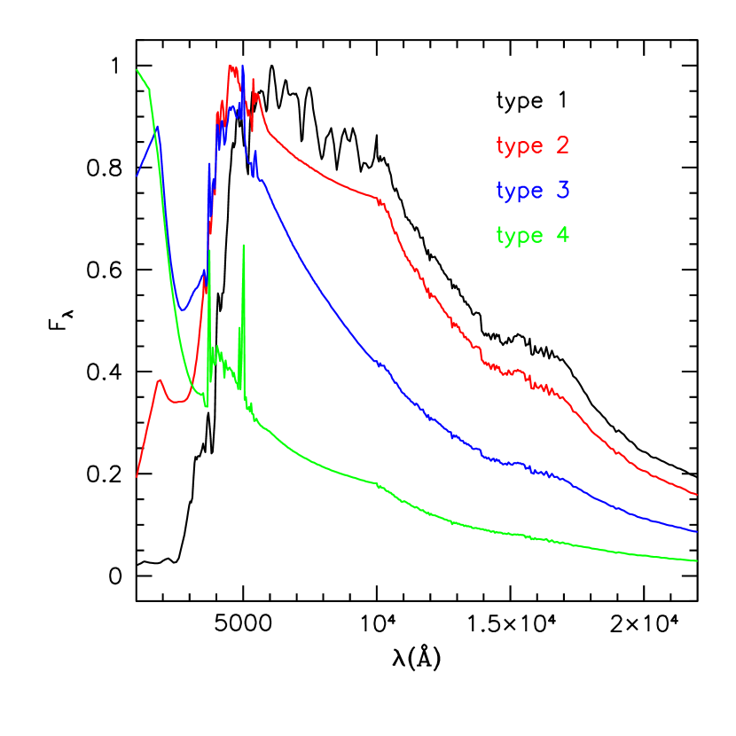
Figure 1: Spectral-energy distributions used to characterize the galaxies of different spectral type. The galaxies are divided into four principal classes: ellipticals/S0 (type 1), early spirals (type 2), late spirals (type 3) and irregulars (type 4). The wavelengths are given in $\AA$, while flux is arbitrary.

The luminosity function for each spectral type and redshift bin is of the form

$$\phi(M)dM = 0.4\phi^{\star}\ln{10}\left(10^{0.4(M^{\star}-M)}\right)^{\alpha+1}\cdot$$ (2)

$$\cdot\exp{\left(-10^{0.4(M^{\star}-M)}\right)}dM\;.$$

It gives the number of galaxies per unit magnitude and per cubic Mpc (Schechter, 1976). The characteristic absolute magnitude $M^{\star}$, the characteristic density $\phi^{\star}$ and the slope $\alpha$ are determined by fitting the observed magnitude distributions of galaxies with the same spectral type and with spectroscopic redshift in the interval between $z_{\rm min}$ and $z_{\rm max}$. We use the values reported in Table 3 of Zucca et al. (2006) for the rest frame B-band (Johnson B filter). The galaxies used in the simulations are generated such as to reproduce the observed luminosity functions in this reference band. The magnitudes in the other bands are easily calculated by using the previous SEDs, suitably normalized such as to assign the correct luminosity in the B-band, and by convolving them with the appropriate filter curves.

The luminosity functions for different morphological types exist for galaxies up to $z=1.5$. For higher redshifts, we adopt the luminosity functions published by Ilbert et al. (2005) and by Paltani et al. (2007) and we extrapolate the fractions of ellipticals, spirals and irregulars from those observed at lower redshift. In particular at $z\gtrsim 2$ we assume that only $5\%$ of the galaxies are ellipticals or S0, while the vast majority of them are spirals and irregulars.

Certainly, important assumptions are made in the process of generating the population of galaxies filling the light cones. First, the VVDS is limited to $I$-magnitude 24 (AB magnitude). Thus, the faint tail of the distribution of galaxy luminosities is extrapolated from a fit performed on brighter galaxies. Second, the absolute magnitudes in bands different from the reference B-band are calculated by adopting a limited number of SEDs. Third, as explained earlier, we can use luminosity functions per different spectral types only at $z<1.5$. For larger redshifts, we must use a single luminosity function and extrapolate from lower redshift the fractions of galaxies with a given SED.

Although it is natural to expect a dominant fraction of irregulars and spirals at high redshift, our procedure may lead to significant errors especially when simulating deep observations. In order to check and validate our methods, we make the following test. We generate a population of galaxies as described above and compare the number counts per magnitude bin and squared arcmin to those measured in the deep observations like the HUDF. We find a good agreement between the number counts independent of the band selected for the experiment. For example, we show in the left panel of Fig. 2 the comparison between our prediction based on the VVDS luminosity functions (solid line) and the HUDF (dotted line) in the $z$-band (F850LP filter on board the Hubble telescope). Although the selected band is much redder than the reference band and the size of the HUDF is rather small, the curves are almost perfectly superposed, confirming the reliability of our results despite the assumptions made.

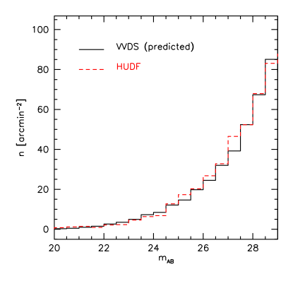
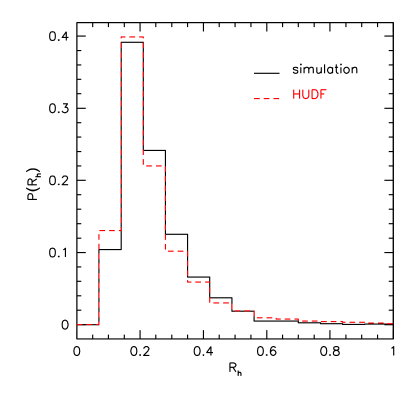
Figure 2: Left panel: Number counts per apparent magnitude bin and squared arcmin predicted by our method (solid line) and observed in the HUDF (dotted line). Magnitudes are given in the $z$-band. Right panel: probability distributions of the galaxy half-light radii in the HUDF (dashed histogram) and in a field simulated with Skylens (solid histogram).

2.2 Galaxy surface-brightness distributions

The light emission from galaxies falling into the telescope field of view is modelled using shapelet functions. This approach has been used by Massey et al. (2004), although using a different shapelet decomposition method. According to Refregier (2003), the galaxy two-dimensional surface-brightness distribution, $I(\@vec{x})$, can be approximated by a summation over a set of basic functions,

$$I(\@vec{x})=\sum_{n_{1},n_{2}=0}^{\infty}I_{\@vec{n}}B_{\@vec{n}}(\@vec{x}-\@vec{x}_{c};\beta)\;,$$ (3)

where $\@vec{x}_{c}$ indicates the galaxy centroid, $\@vec{x}=(x_{1},x_{2})$ is a two-dimensional vector, and $\@vec{n}=(n_{1},n_{2})$. The basic functions $B_{\@vec{n}}(\@vec{x};\beta)$ are called shapelets and have the form

$$B_{\@vec{n}}(\@vec{x},\beta)=\beta^{-1}\phi_{n_{1}}(\beta^{-1}x_{1})\phi_{n_{2}}(\beta^{-1}x_{2})\;,$$ (4)

where the one-dimensional functions $\phi_{n}(x)$ are related to the Gauss-Hermite polynomials, $H_{n}(x)$,

$$\phi_{n}(x)=[2^{n}\pi^{1/2}n!]^{-1/2}H_{n}(x)\exp(-x^{2}/2)\;.$$ (5)

The parameter $\beta$ defines the scale of the galaxy image. The coefficients $I_{\@vec{n}}$ properly weight the contribution of each shapelet function to the surface-brightness of the galaxy and are given by

$$I_{\@vec{n}}=\int{\rm d}^{2}xI(\@vec{x})B_{\@vec{n}}(\@vec{x};\beta)\;.$$ (6)

Basic photometric information about the galaxy is readily derived from the shapelet coefficients. For example, the total flux $I$ is given by

$$I=\pi^{1/2}\beta\sum_{n_{1},n_{2}}^{\rm even}2^{\frac{1}{2}(2-n_{1}-n_{2})}\left(\begin{array}[]{c}n_{1}\\ n_{1}/2\end{array}\right)^{1/2}\left(\begin{array}[]{c}n_{2}\\ n_{2}/2\end{array}\right)^{1/2}I_{\@vec{n}}\;,$$ (7)

and the rms radius $r_{I}$, defined as $r_{I}^{2}\equiv\int{\rm d}^{2}xx^{2}I(\@vec{x})/I$, is given by

$$r_{I}^{2} = \pi^{1/2}\beta^{3}I^{-1}\sum_{n_{1},n_{2}}^{\rm even}2^{\frac{1}{2}(4-n_{1}-n_{2})}(1+n_{1}+n_{2})$$ (12)

$$\times\left(\begin{array}[]{c}n_{1}\\ n_{1}/2\end{array}\right)^{1/2}\left(\begin{array}[]{c}n_{2}\\ n_{2}/2\end{array}\right)^{1/2}I_{\@vec{n}}\;.$$

The shapelet decomposition has proven to be a powerful technique for image anaysis (see e.g. Melchior et al., 2007; Massey et al., 2007b; Goldberg & Bacon, 2005). Among the many applications, Kelly & McKay (2004) have shown that it can be applied to morphological classification. In fact, they find that galaxies of different morphological types separate well in shapelet space. On the other hand, Massey et al. (2004) showed that an infinite number of synthetic galaxy images can be easily created from a set of shapelet coefficients obtained from decomposing real galaxies. Following these ideas, we aim at using real shapelet decompositions to characterize galaxy morphologies in our simulator. In detail, we proceed as follows:

1. we use the newly developed code by Melchior et al. (2007) for shapelet-decomposing the images of $\sim 3000$ galaxies from the GOODS HST/ACS data (Giavalisco et al., 2004). For each galaxy, the code provides the best fit set of coefficients, $I_{\@vec{n}}^{\rm GOODS}$, together with their errors, and the scale parameter, $\beta^{\rm GOODS}$;

2. for about half of the galaxies in the database a spectral classification is available, which allows us to distinguish between morphological types and to assign a SED to each galaxy. For those galaxies which have no classification, we assume that they are irregulars or late spirals, since they are typically faint and distant blue objects. Based on this classification, the galaxy decompositions are divided into four catalogs corresponding to the SEDs described in Sect. 2.1;

3. aiming at generating a galaxy of type M, one entry from the corresponding catalog is randomly chosen. Since our catalogs contain a limited number of galaxies, which may be smaller than the number of galaxies to be generated in the simulation, replications of the same galaxy may occur. To avoid that, whenever a galaxy is chosen, we slightly change the values of the shapelet coefficients (within their errors) to obtain a new, slightly different, galaxy image;

4. the galaxy image is finally rescaled on the basis of the input flux. From the decompositions contained in our shapelet database we build an empirical relation between the scale parameter and the flux. Then, we use this relation and its dispersion to draw the scale parameter $\beta$ that corresponds to the input flux $I$. Eq. 7 however states that $I\propto\beta I_{\@vec{n}}$. Thus, to ensure consistency, when scaling a GOODS galaxy with scale parameter $\beta_{0}$ and flux $I_{0}$ to one with scale parameter $\beta$ and observed flux $I$, we also adjust its shapelet coefficients by multiplying them by $(I/I_{0})(\beta_{0}/\beta)$. In order to verify the reliability of our method, we compared the size distribution of simulated galaxies with that observed in the HUDF. The probability distribution functions of the half-light radii (as outputted by SExtractor, Bertin & Arnouts (1996)) in the simulated and in the observed HUDF are shown in the right panel of Fig 2. For the observed HUDF, we refer to the catalog published by Beckwith et al. (2006). The simulated images have been analyzed consistently, i.e. by adapting the SExtractor parameters to those used in the observations. Clearly, the distributions are very similar, although the half-light radii tend to be slightly larger in the simulation (median $R_{h}=0.211"$) than in the real observation (median $R_{h}=0.204"$). An even more accurate result will be achieved when our shapelet database is extended using deeper observations, including a larger number of low-flux sources;

5. once a set of coefficients and a scale parameter have been defined, they can be used to generate a new galaxy surface-brightness distribution. In order to ensure random orientations, we rotate by a random angle $\psi\in[0,\pi]$

In Fig. 3 we show an example illustrating the generation of syntetic galaxies out of a real GOODS galaxy. In the left panel, we show a spiral galaxy from GOODS. The galaxy is decomposed into shapelets with maximum order $n_{1}=n_{2}=9$. The decomposition is then used to reconstruct the original galaxy image in the central panel. Finally, a second galaxy surface brightness distribution is generated from the same decomposition but after having slightly changed the values of the shapelet coefficients. As explained above, the coefficients and the scale parameter may also be rescaled to change the output flux of the sources, allowing us to create synthetic galaxies in arbitrary numbers. Moreover, as it will be shown later, using shapelets permits us to easily incorporate lensing effects in the simulations. All images already contain several sources of noise that will be discussed in the following sections.

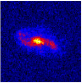
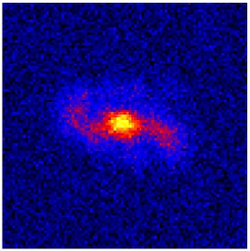
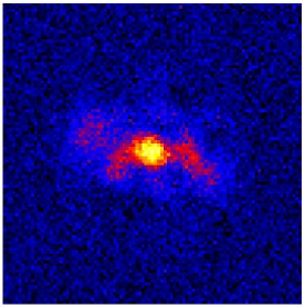
Figure 3: Example of generation of synthetic galaxies with shapelets. In the left panel the original image of a GOODS galaxy is shown. The galaxy is decomposed in $9\times 9$ shapelets and reconstructed in the central panel. A second galaxy is then generated from the same shapelet decomposition by slightly modifying the coefficients and displayed in the right panel. The same color scale is used for all three images. To reproduce the background and the noise properties of the image in the left panel, we have simulated an observation with HST/ACS (filter F850LP, $t_{\rm exp}=10600$ sec). Each frame is $2.9^{\prime\prime}$ on a side.

2.3 Observing deep fields

Once a number of galaxies have been generated, having a luminosity, a SED, a redshift and a shape assigned, we can simulate observations for a particular instrumental set-up. This implies calculating the number of photons coming from a patch of the sky which are collected by each element of the CCD camera, after the light has passed through a sequence of mirrors and filters, and, eventually, through the Earth’s atmosphere.

2.3.1 Photon counts

For the implementation of our simulator, we follow the prescriptions given by Grazian et al. (2004) in the construction of the Large-Binocular-Telescope Camera Image Simulator (LBCSIM). Given a telescope of diameter $D$, the number of photons collected by the CCD pixel at $\@vec{x}$ in the exposure time $t_{\rm exp}$, from a source whose surface brightness is $I(\@vec{x})$ (erg s^-1cm^-2Hz^-1arcsec^-2), is

$$n_{\gamma}(\@vec{x})=\frac{\pi D^{2}t_{\rm exp}p^{2}}{4h}I(\@vec{x})\int\frac{T(\lambda)}{\lambda}{\rm d}\lambda\;,$$ (13)

where $p$ is the pixel size in arcsec, $h$ is the Planck constant and $T(\lambda)$ is the total transmission, which is given by the product of the atmospheric extinction for a given airmass, $A^{\prime}(\lambda)=10^{-0.4\cdot{\rm airmass}\cdot A(\lambda)}$ (airmass$=0$ for observations from space), and the efficiencies of the CCD, $C(\lambda)$, of the filter, $F(\lambda)$, of the mirror, $M(\lambda)$, and of the optics $O(\lambda)$,

$$T(\lambda)=A^{\prime}(\lambda)\cdot C(\lambda)\cdot F(\lambda)\cdot M(\lambda)\cdot O(\lambda)\;.$$ (14)

The number of photons is converted into a number of ADUs (Astronomical Data Units) by dividing by the gain $g$ of the CCD:

$$ADU(\@vec{x})=\frac{n_{\gamma}(\@vec{x})}{g}\;.$$ (15)

2.3.2 Lensing effects

Lensing by intervening matter along the line of sight is applied by mapping the CCD pixel coordinates using the lens equation 1. The pixel at $\@vec{x}$ is now connected to the position $\@vec{y}$ on the plane where the galaxy surface brightness is assigned. Then, the surface brightess at $\@vec{y}$ is converted into ADUs using Eqs. 13 and 15 and the computed value is assigned to the pixel at position $\@vec{x}$ on the CCD:

$$ADU_{\rm lensed}(\@vec{x})=ADU[\@vec{y}(\@vec{x})]\;,$$ (16)

Note that in the strong lensing regime one coordinate $\@vec{y}$ can correspond to more than one pixel coordinate $\@vec{x}$.

The application of Eq. 16 in the case of arbitrary pixel scales involves two steps. First, since the deflection angles may be determined on a grid whose point positions generally differ from those of CCD pixels, the deflection angle map must be interpolated at each pixel position, $\@vec{x}$. We use a bi-cubic interpolation scheme, which works well provided the spatial resolution of the virtual CCD is not too large compared to that of the input deflection angle map. Second, since the galaxies are distributed in redshift, the deflection angles must be rescaled by the factor $D_{\rm ls}/D_{\rm s}$ appearing in Eq. 1 for each source. Especially when simulating observations of large fields, this operation may become time consuming because of the large number of pixels and sources. To shorten the calculations, we bin the sources in redshift and project all the galaxies in a given redshift bin on a single plane. For example, we assign to all galaxies at a redshift between $z_{\min}$ and $z_{\rm max}$ the redshift $z_{\rm s}=(z_{\min}+z_{\rm max})/2$. By changing the size of the redshift bins, one can increase or decrease the number of source planes. All sources falling into the same redshift bin can then be processed at the same time, saving a considerable amount of computational time.

Note that using the shapelet formalism for representing the source galaxies allows to apply weak lensing transformations through relatively simple operators acting on the shapelet states. For first order lensing, Refregier (2003) shows that the transformation can be written as

$$ADU_{\rm lensed}(\@vec{x})\simeq\left[1+\kappa(\@vec{x})\hat{K}+\gamma_{i}(\@vec{x})\hat{S}_{i}\right]ADU(\@vec{x})\;,$$ (17)

where $\kappa$ and $\@vec{\gamma}=(\gamma_{1},\gamma_{2})$ are the convergence and the shear, respectively. The operators $\hat{K}$ and $\hat{S}$ can be expressed in terms of the raising and lowering operators for the quantum harmonic oscillator as

$$\hat{K} \equiv 1+\frac{1}{2}\left[\hat{a}_{1}^{{\dagger}2}+\hat{a}_{2}^{{\dagger}2}-\hat{a}_{1}^{2}-\hat{a}_{2}^{2}\right]$$ (18)

$$\hat{S}_{1} \equiv \frac{1}{2}\left[\hat{a}_{1}^{{\dagger}2}-\hat{a}_{2}^{{\dagger}2}-\hat{a}_{1}^{2}+\hat{a}_{2}^{2}\right]$$ (19)

$$\hat{S}_{2} \equiv \hat{a}_{1}^{{\dagger}2}\hat{a}_{2}^{{\dagger}2}-\hat{a}_{1}^{2}\hat{a}_{2}^{2}$$ (20)

Thus, by using these formulas in combination with Eqs. 3, 13 and 15, the lensing distortion can be expressed in terms of transformations of the shapelet coefficients, $I_{\@vec{n}}$.

2.3.3 Convolution with the PSF and seeing

Several sources of noise can then be added to the image to resemble real observational conditions.

First, the images can be convolved with the instrumental point-spread-function (PSF):

$$I^{\prime}(\@vec{x})=\int{\rm d}^{2}x^{\prime}I(\@vec{x}^{\prime})F(\@vec{x}-\@vec{x}^{\prime})\;.$$ (21)

The convolution can be done in two ways. In analogy to the galaxy images, a given PSF model, $F(\@vec{x})$, can be decomposed into shapelets. Convolution is entirely analytically possible in shapelet space, given the invariance of the shapelet functions under Fourier transformations. The full formalism is explained in Refregier (2003). This approach has been used by Massey et al. (2007a) for image simulations. The method is efficient for doing convolutions involving un-lensed or weakly lensed galaxies, i.e. galaxies with known shapelet decompositions. For very distorted galaxies, like in the strong lensing regime, applying this method would require to further shapelet-decompose the lensed images, whose shapelet coefficients cannot be easily derived from the un-lensed ones (for example using Eq.17). Thus, this would lead to a loss of computational efficiency. For this reason, when simulating fields including strong lensing features, we opt for applying standard FFT techniques for doing convolution operations.

This approach allows to simulate the shape of the PSF very realistically. However, the PSF is unique for the whole image, i.e. local variations of the PSF shape were not mimicked so far.

In weak lensing applications, the PSF needs to be corrected in order to extract the lensing signal from the source ellipticities. Residuals in the PSF corrections, due for example to the above mentioned variations of the PSF shape are one of the major sources of error (see e.g. Rhodes et al., 2007).

To take this into account in our simulations, we propose the following approach to model the PSF. The general idea is that distortions of the PSF shape can be described as an additional “lensing” effect. Anisotropies cause the images of stars to acquire irregular shapes, being stretched along some particular directions as if an external shear was applied. Such an external shear can be characterized by a power spectrum, whose amplitude defines the intensity of the anisotropies and whose shape characterizes the spatial scales over which it varies.

Let the shear power spectrum be $P_{\gamma}$. We can link the power spectrum to a source potential power spectrum using standard definitions. Since the components of the shear are combinations of the second derivatives of the lensing potential,

$$\gamma_{1} = \frac{1}{2}\left(\frac{\partial^{2}\psi}{\partial x_{1}^{2}}-\frac{\partial^{2}\psi}{\partial x_{2}^{2}}\right)$$ (22)

$$\gamma_{2} = \frac{\partial^{2}\psi}{\partial x_{1}\partial x_{2}}\;,$$ (23)

in the Fourier space we have that

$$\hat{\gamma}_{1} = \frac{k_{1}^{2}-k_{2}^{2}}{2}\hat{\psi}$$ (24)

$$\hat{\gamma}_{2} = k_{1}k_{2}\hat{\psi}\;,$$ (25)

where the hat denotes Fourier transforms and $\@vec{k}=(k_{1},k_{2})$ is the wave vector. The power spectrum of the source potential is thus

$$P_{\psi}=\frac{4}{k^{4}}P_{\gamma}\;.$$ (26)

Using this formalism, the distortions of the PSF can be introduced by applying additional lensing to the images already convolved with a PSF function. Given a potential $\psi$, the corresponding deflection angle field is

$$\@vec{\alpha}=\@vec{\nabla}\psi\;,$$ (27)

and in Fourier space

$$\alpha_{1} = -\mathrm{i}k_{1}\hat{\psi}$$ (28)

$$\alpha_{2} = -\mathrm{i}k_{2}\hat{\psi}\;.$$ (29)

Thus, the power spectra of the two components of the deflection angle are:

$$P_{\alpha_{1}} = k_{1}^{2}P_{\psi}=\frac{k_{1}^{2}}{k^{4}}P_{\gamma}$$ (30)

$$P_{\alpha_{2}} = k_{2}^{2}P_{\psi}=\frac{k_{2}^{2}}{k^{4}}P_{\gamma}\;.$$ (31)

For simplicity, we assume that $P_{\gamma}$ is a Gaussian,

$$P_{\gamma}(k)=A_{\gamma}\exp{-\frac{k^{2}}{k_{\rm cut}^{2}}}\;,$$ (32)

whose amplitude is $A_{\gamma}$ and whose characteristic scale is $k_{\rm cut}$. This last parameter sets the scales over which spatial variations of the PSF shape occur.

Thus, we use $P_{\gamma}$ to generate maps of the deflection angle components. For doing that we assume that these maps are Gaussian, with zero mean and variance defined by the amplitude of the input power spectrum. The deflection angles are used to lens the images as explained in the previous section.

When simulating ground based observations, seeing is simulated by further convolving the image with a Gaussian $G$ of size $\sigma$:

$$I_{\sigma}(\@vec{x})=\int{\rm d}^{2}x^{\prime}I^{\prime}(\@vec{x}^{\prime})G(\@vec{x}-\@vec{x}^{\prime})\;.$$ (33)

In Fig. 4 we show some examples. In the top panel, an array of stars convolved with an isotropic PSF with Gaussian profile and FWHM of $0.6"$ (including seeing) is shown. The angular separation of the stars along the $x$ axis is $10"$. In the middle panel, we introduce variations of the PSF shape on scales of $\sim 1"$. The amplitude of the distortions is intentionally quite large and correspond to $A_{\gamma}=0.9$. Instead, in the bottom panel we mimic a PSF that slowly varies on scales of $\sim 15"$. These examples show that by properly choosing the parameters $A_{\gamma}$ and $k_{\rm cut}$ a suitable level of noise in the PSF can be added.

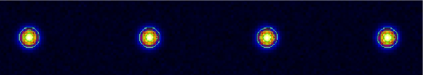
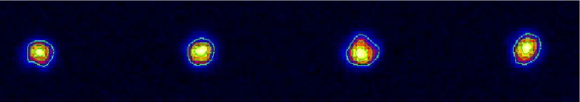
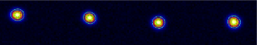
Figure 4: Images of an array of stars observed with an LBT-like telescope. The angular separation between the stars is $10"$ along the $x$ axis. In the top panel, an isotropic PSF (FWHM=$0.6"$) is mimicked. In the middle panel, anisotropies varying on scales of $\sim 1"$ are included. In the bottom panel we simulate larger-scale variations of the PSF shape on scales of $\sim 15"$.

2.3.4 Sky background and photon noise

The number of ADUs per pixel from the sky background are given by

$$ADU_{\rm sky}=\frac{\pi D^{2}t_{\rm exp}p^{2}}{4hg}\int\frac{T(\lambda)S(\lambda)}{\lambda}{\rm d}\lambda\;,$$ (34)

where $S(\lambda)$ is the sky flux per square arcsec at a given wavelength and $T(\lambda)$ is calculated now at ${\rm airmass=0}$. The sky flux is modeled differently for observations from the ground and from space. For ground based observations, we use different night sky spectra according to the different phases of the moon. The spectra are those used in Grazian et al. (2004). They correspond to 0, 3, 7, 10 and 14 days after the dark moon. For simulating the sky as seen from the space, we adopt several spectra of zodiacal light, representing the typical variations of the zodiacal background radiation and of the earthshine (Giavalisco et al., 2002).

Photon noise is assumed to be Poissonian. For each pixel the noise (in ADUs) is generated by adding random deviates with Gaussian probability distribution of mean zero and width

$$\sigma_{N}(\@vec{x}) = \left\{n_{\rm exp}\left(\frac{RON}{g}\right)^{2}+\frac{ADU(\@vec{x})+ADU_{\rm sky}}{g}\right.$$ (35)

$$+\left.\left(f+\frac{a^{2}}{n_{\rm exp}^{2}}\right)[ADU(\@vec{x})+ADU_{\rm sky}]^{2}\right\}^{1/2}\;.$$

In the previous formula $RON$ is the read-out noise of the chip, $n_{\rm exp}$ is the number of exposures, $a$ is the flat-field term, which we fix at $a=0.005$ following Grazian et al. (2004). The term $f$ indicates the flat-field accuracy, which is determined by the number of flat-field exposures and by the level of the sky background as

$$f=(N_{ff}\cdot B\cdot g)^{-1}\;.$$ (36)

A more detailed explanation of these formulas is given in Section 4.2 of Grazian et al. (2004).

2.3.5 Producing the images

By properly setting the total efficiency (using the correct efficiency curves for optics, mirrors and CCDs) observations from several instruments can be simulated. As an example, we show in Fig. 5 how the same galaxy displayed in the central panel of Fig. 3 would appear when observed with the LBT with a diffraction limit PSF (left panel) and in bad seeing conditions ($\sigma=1.2^{\prime\prime}$; right panel). The exposure time is $2000$ sec with ${\rm airmass}=1$. The pixel size of the LBT camera is $0.224^{\prime\prime}$, in contrast to the $0.03^{\prime\prime}$ of HST/ACS (after drizzling). The spiral structure of the galaxy is thus not resolved by LBT. Seeing blurs the image, destroying most of the remaining morphological information.

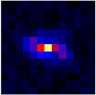
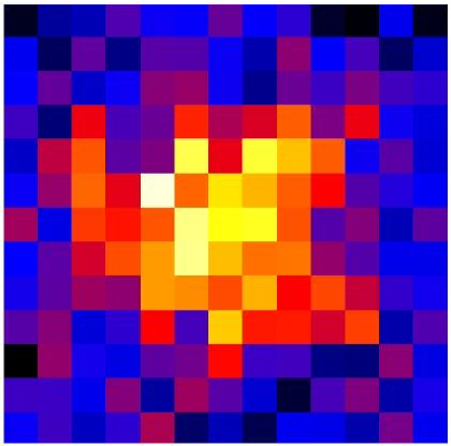
Figure 5: The same galaxy displayed in the central panel of Fig. 3 is shown here as it should be observed in the $I$-band by LBT with a diffraction limited PSF (left panel) and in bad seeing conditions ($\sigma=1.2^{\prime\prime}$, right panel). The exposure time is $t_{\exp}=2000$ sec and the airmass is 1. The scale of each frame is $2.9^{\prime\prime}$.

Combining several galaxies into the same field, we are able to produce artificial galaxy fields. One example is given in Fig. 6, where we simulate a deep field of $1^{\prime}\times 1^{\prime}$ observed with the HST/ACS with an exposure time of $10600$ sec. In this simulation, no lensing effects have been included. As demonstrated here, using our procedure for generating artificial galaxies we can produce very realistic simulated images of the sky.

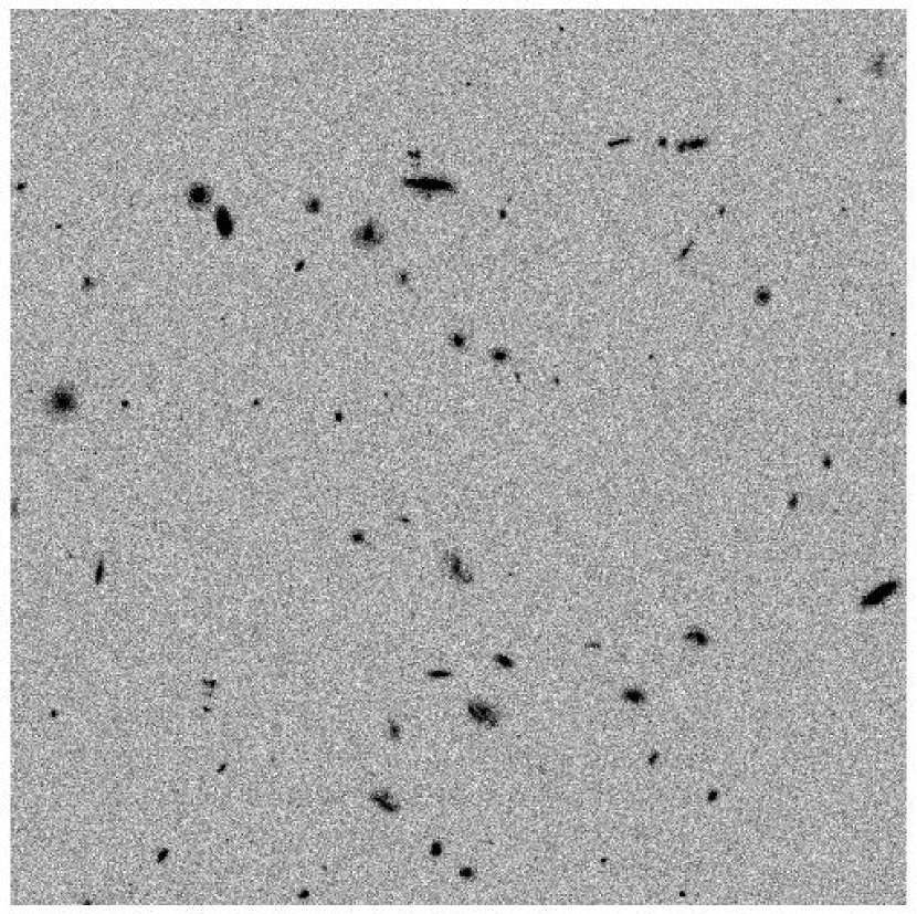
Figure 6: Simulation of a deep field observed by HST/ACS in the $z$-band. The exposure time is $t_{\rm exp}=10600$ sec and the field of view is $1^{\prime}\times 1^{\prime}$.

2.3.6 Foregrounds

The light emission from foreground galaxies can be included in simulated images adopting the same procedure employed for background sources. We note that cluster galaxies in particular represent a potential problem for lensing analyses. For weak lensing studies, misidentification of cluster members as background sources can bias the shear measurements. In addition the bright galaxies concentrated near the cluster centre (which corresponds to the strong lensing regime) complicate the detection of lensed sources.

In order to include realistic galaxy clusters in our simulated images, we have used results from a semi-analytic model of galaxy formation coupled to a cluster N-body re-simulation. The semi-analytic model used in this study is described in De Lucia & Blaizot (2007) and we refer to the original study (and references therein) for more details about the physical processes modelled. The model is used to generate a catalogue containing positions and luminosities of model galaxies at different redshifts. This information is used to simulate galaxy images as described in the previous section. As in previous work, we determine the morphology of our model galaxies by using the B–band bulge–to–disc ratio together with the observational relation by Simien & de Vaucouleurs (1986) between this quantity and the galaxy morphological type.

An example of a simulated observation of a galaxy cluster is shown in Fig. 7. The cluster is at redshift $z\sim 0.3$. It is observed with HST/ACS in the $z$-band with an exposure time of $1000$ sec. The cluster is dominated by some very bright galaxies ($L\sim 10^{12}L_{\odot}$) in the central part. They are expected to complicate significantly the observability of lensing features, in particular radial arcs, occurring near the cluster center.

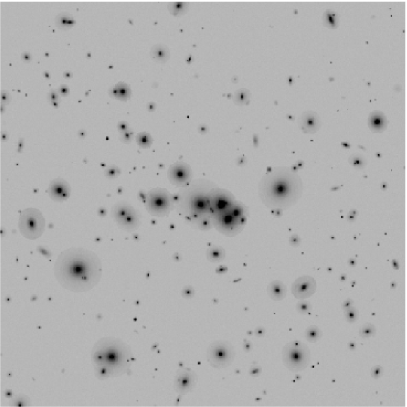
Figure 7: Virtual observation in the $z$-band by HST/ACS of a galaxy cluster at $z\sim 0.3$. The exposure time is $t_{\rm exp}=1000$ sec and the field of view is $100"\times 100"$. The spatial distribution and luminosities of the cluster galaxies have been obtained from semi-analytic models. The lensing effects are disabled in this simulation.

3 Applications of the method

In this Section, we discuss one possible application of our simulator, i.e. simulating gravitational arcs in the center of galaxy clusters. Then we apply some techniques, that can be used also in real observations, to measure the properties of the arcs detected in the images.

3.1 The cluster model

The cluster used in this paper is one the clusters previously studied by Dolag et al. (2005). Its lensing properties were investigated also by Puchwein et al. (2005) and by Meneghetti et al. (2007). A detailed description of the simulation can be found in these papers. Its reference name is $g1$. Although several versions of this cluster exist that include the treatment of the gas component with several physical processes, we have chosen to use for the present paper the simplest simulation, where the cluster contains only dark matter particles.

The halo has a mass of $\sim 1.4\times 10^{15}\>h^{-1}M_{\odot}$ (resolved by more than a million particles within the virial region), thus it represents a very massive and efficient strong lens at $z=0.3$. We have chosen this redshift because it is close to where the strong lensing efficiency of clusters is the largest for sources at $z_{\rm s}\gtrsim 1$ (Li et al., 2005).

Although we are investing the lensing property of this halo only at at $z=0.3$, during the simulation 92 time slices were saved from redshift $60$ to $0$. These are equispaced in time. For each snapshot, we computed group catalogues and their embedded substructures using a standard friends-of-friends algorithm with a linking length of 0.2 in units of the mean particle separation, and a modified version of the algorithm SUBFIND (Springel et al., 2001) that was extended for future applications to hydro-simulations. Substructure catalogues were then used to construct merger history trees as described in Springel (2005) and De Lucia & Blaizot (2007). These merger trees are the basic input needed for the semi-analytic model described in Sect. 2.3.6.

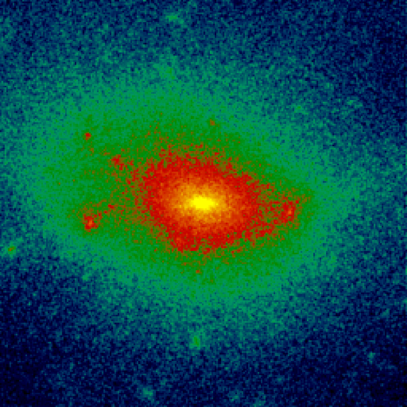
Figure 8: Surface density map of cluster $g1$ corresponding to projecting the cluster along the $z$-axis of the simulation box. The side-length of the image is $1.5\,h^{-1}$Mpc comoving (corresponding to $\sim 372"$).

The surface density map corresponding to one projection of the cluster is shown in Fig. 8. The size of the image is $(1.5\,h^{-1}$Mpc)². The inner region appears quite elliptical and devoid of large substructures. Secondary massive clumps of matter are located at distances $\gtrsim 400\,h^{-1}$kpc from the cluster center.

3.2 Calculations of deflection angles

Ray-tracing simulations are carried out using the technique described in detail in several earlier papers (e.g. Bartelmann et al. 1998; Meneghetti et al. 2000).

We select a cube of $3\,h^{-1}$Mpc comoving side length, centred on the halo centre and containing the high-density region of the cluster. The particles in this cube are used for producing a three-dimensional density field, by interpolating their position on a grid of $1024^{3}$ cells using the Triangular Shaped Cloud method (Hockney & Eastwood, 1988). Then, we project the three-dimensional density field along the coordinate axes, obtaining three surface density maps $\Sigma_{i,j}$, used as lens planes in the following lensing simulations.

The lensing simulations are performed by tracing a bundle of $2048\times 2048$ light rays through a regular grid, covering the central sixteenth of the lens plane. This choice is driven by the necessity to study in detail the central region of the cluster, where critical curves form, taking into account the contribution from the surrounding mass distribution to the deflection angle of each ray.

Deflection angles on the ray grid are computed as follows. We first define a grid of $256\times 256$ “test” rays, for each of which the deflection angle is calculated by directly summing the contributions from all cells on the surface density map $\Sigma_{i,j}$,

$$\@vec{\alpha}_{h,k}=\frac{4G}{c^{2}}\sum_{i,j}\Sigma_{i,j}A\frac{\@vec{x}_{h,k}-\@vec{x}_{i,j}}{|\@vec{x}_{h,k}-\@vec{x}_{i,j}|^{2}}\;,$$ (37)

where $A$ is the area of one pixel on the surface density map and $\@vec{x}_{h,k}$ and $\@vec{x}_{i,j}$ are the positions on the lens plane of the “test” ray ($h,k$) and of the surface density element ($i,j$). We avoid the divergence when the distance between a light ray and the density grid-point is zero by shifting the “test” ray grid by half-cells in both directions with respect to the grid on which the surface density is given. We then determine the deflection angle of each of the $2048\times 2048$ light rays by bi-cubic interpolation between the four nearest test rays.

3.3 Observations

For simulating observations of our numerical cluster, we consider an instrument with the characteristics of the planned space telescope DUNE (Dark Universe Explorer; http://www.dune-mission.net). This mission was recently proposed to ESA within its ”Cosmic Visions” programme. It is targetted at studying the dark components of the universe with a wide field imager, in particular through weak lensing. However, thanks to the good spatial resolution, the panoramic field of view ($0.5$ square degrees) and high sensitivity, this instrument will be extremely useful for many other studies including strong lensing, galaxy formation and evolution, baryonic acoustic oscillations and even planet searches.

The motivation for adopting a future instrument for our virtual observation is twofold. On one hand, we would like to illustrate that the simulator is a powerful tool for testing techniques that are commonly applied to observational data. On the other hand, we would like to highlight that codes like this can help to define the scientific tasks that can be fulfilled by future missions.

DUNE is planned to have a mirror diameter of 1.2 meters, a spatial resolution of $0.10"$/pixel in the visible and a total efficiency close to $\sim 70\%$. During the proposal preparation, three broad-band filters where used, namely a $u+g+r$ ($ugr$), a $r+i+z$ ($riz$) and a $i+z+y$ ($izy$) filter. In the proposed version, DUNE will not provide 3 bands in the visible. On the contrary, there will be one filter in the visible ($riz$) and 3 filters in the NIR ($Y,J,H$). The tests that are discussed below have been performed using the $riz$ filter. Just for the purpose of illustrating the capabilities of the simulator for mimicking observations in multiple bands, we used the $ugr$ and the $izy$ filters (see Fig. 10 below). The throughputs that we assume, including the quantum efficiency of the detector and the optical design, are shown in Fig. 9. The PSF is expected to have a FWHM of $0.23"$ with ellipticity smaller than $6\%$.

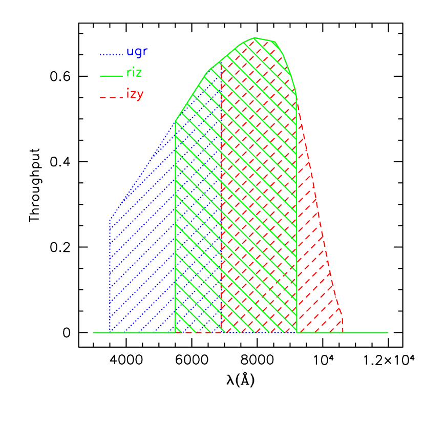
Figure 9: Throughputs assumed in carrying out the simulations with the DUNE satellite. Three broad-band filters are used: $ugr$ (dashed lines), $riz$ (solid lines), $izy$ (courtesy of A. Amara, J. Rhodes and the DUNE collaboration members). Note that the figure does not reflect the final choice for the filters to be mounted on DUNE (see text for more details).

A virtual observation of the inner $100"\times 100"$ region of cluster $g1$ is shown in Fig. 10. It is a composite $ugr$, $riz$ and $izy$ image, corresponding to an exposure time of $1000$ sec. In these tests, we assume an exposure time of $1000$ seconds, although it has been proposed that DUNE exposures will be longer ($1500$ seconds). The galaxies were drawn from our the shapelet library, as explained earlier. In order to facilitate the formation of strong lensing features, we intentionally placed seven ”test” galaxies close to the caustics of the lens. They are shown in the left panel of Fig. 11, where we run a simulation without the foreground lens and we zoom over the region where the caustics are located. The caustics are also shown in blue. For simplicity, we assume that the ”test” sources are all at $z_{s}=1.5$. Two galaxies, labeled A and B, are placed very close to the cusps of the tangential caustic, thus they are expected to produce extended cusp arcs. Two other galaxies (F,G) are placed along the radial caustic and their images will be radially elongated arcs. The remaining ”test” sources (C,D,E) are located along the fold of the tangential caustic, thus they should be lensed to form fold arcs. The lensed images are presented in the central panel of Fig.11.

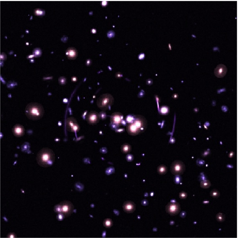
Figure 10: Composite $ugr$+$riz$+$izy$ image of the cluster $g1$. Several strong lensing features are present in the image. The FOV size is $100"\times 100"$.

Some of the arcs, and especially the radial ones, are partially or totally hidden by the light of the foreground galaxies, as can be seen in Fig.10. On the basis of the cluster merger tree, the semi-analytic models predict the presence of a very bright galaxies near the cluster center. These render accurate measurements of arcs shapes behind them problematic. In real cases, these galaxies should be removed (see e.g. Sand et al., 2004). Thus, we subtract the foreground galaxies from the image by fitting their surface brightness profiles with Sersic profiles. This can be done with a suitable software like GALFIT (Peng et al., 2002).

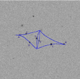
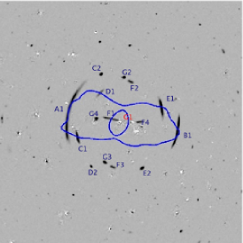
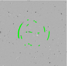
Figure 11: Left panel: positions of the sources relative to the caustics of the lens. The image is $25"\times 25"$ wide. Central panel: $riz$ image of the cluster g1 after subtracting the cluster galaxies using magnitude and size cuts (see text for more details). The size of the image is $100"\times 100"$. The images of the sources in the left panel are indicated by the letters, followed by numbers corresponding to image multiplicity. The image G1 is not visible, but we mark in red the position where it should be. Right panel: the points belonging to the lensed images are marked in green.

We show the image after removing the foreground light in the central panel of Fig. 11. Superposed to the lensed field, we display the cluster critical lines. Cluster members have been identified by selecting galaxies with magnitude $m_{riz}<22$ and rms radius $r_{I}>0.5"$. Comparing to the input catalogs of cluster members, we find that foreground galaxies were efficiently identified by applying these selection criteria. The images of the ”test” galaxies displayed in the left panel are indicated by letters followed by numbers corresponding to their multiplicity. Note the radial image labeled as G1 (one of the images of source G) is not detectable even after subtraction of the foreground galaxies.

3.4 Arc properties

In some applications of strong cluster lensing, such as arc statistics, it is important to accurately measure the properties of gravitational arcs. Properties like length, width and curvature radius of the images can be used to constrain cosmological parameters (Bartelmann et al., 1998, 2003; Wambsganss et al., 2004; Oguri et al., 2003; Li et al., 2005; Meneghetti et al., 2005; Horesh et al., 2005; Hilbert et al., 2007) but also for determining the inner-structure of galaxy clusters (Sand et al., 2005). In this section we illustrate a procedure to measure the shape of arcs that can be applied to both real and simulated, thus favoring the comparison between observations and simulations.

First, we identify the pixels in the image that belong to the lensed images. To do that, we make local measurements of the sky background and set a limit above which pixels can safely be assigned to the arcs. For avoiding the inclusion of noise, especially where foreground galaxies have been subtracted, we select only pixels above $S/N>5$. The result of this selection is presented in the right panel of Fig. 11. Several images cannot be classified as arcs (for example the images C2, D2, etc), thus we exclude them from the following analysis. We focus on the arcs A1, B1, C1, D1, E1 and F1.

As suggested by Miralda-Escude (1993) (see also Bartelmann et al., 1998; Meneghetti et al., 2000, 2001), we define three characteristic points on the arcs, namely

1. the brightest point, that is likely to be an image of the source center;

2. the point at the largest distance from 1);

3. the point at the largest distance from 2).

In the case of arc A1, these three points are shown in Fig.12. We trace a circle segment through these characteristic points. Its length and curvature radius are identified to the length and the curvature radius of the arc, respectively.

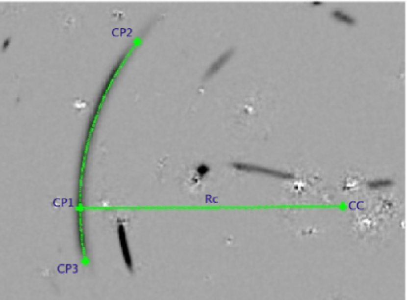
Figure 12: Fit of the arc A1: three characteristic points have been identified on the image (CP1-3), through which a circular segment (CP2-CP3) have been traced. The curvature radius (Rc) and the centre of curvature (CC) of the circular segment define the radius and the centre of the arc.

Measuring the arc width is less simple. Arcs are typically structured, as they originate from mergers of multiple images of the same source. Thus, even in the case of simple, elliptical sources, the width is not constant along the arc. Moreover, arcs form in crowded regions of clusters. As shown in the previous examples, the light from cluster members can influence the detectability of the lensed images or of part of them, thus affecting the measurements of the arc widths and lengths. Cluster galaxies can also alter the shape of arcs by mean of their lensing effects (Meneghetti et al., 2000). Last but not less important, photon noise causes the edges of the images to be irregular.

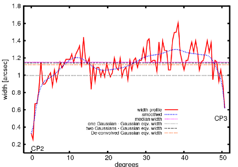
Figure 13: Transversal width profile of arc A1 (red solid line). The blue dotted line shows an interpolation of the profile with a Bezier curve. The horizontal lines correspond to various determinations of the arc width.

The transversal width profile of arc A1 is shown in Fig. 13 (solid line). This has been recovered by making radial scans of the arc along straight lines passing through the center of curvature CC (see Fig. 12) and intercepting the circular segment CP2-CP3 at equi-spaced angular separations. The angle is given in degrees with respect to the line CC-CP2. At each scan, we measure the maximal distance between arc points intercepted by the straight line. Some large scale fluctuations of the width can be recognized, that are caused by mergers of multiple images. To make these large scale modes more visible, we interpolate the profile with a Bezier curve (dotted line) (Knuth, 1986). The profile has several intervals with positive curvature separated by valleys. The valleys are located at the positions where the arc crosses the cluster critical line, as shown in the central panel of Fig 11. They roughly correspond to the regions where multiple images of the source have merged together. Additionally, many other small scale fluctuations are produced by noise. Thus, it appears difficult to define at which position the arc width has to be measured. We propose here to use the median width.

In the case of observations through the Earth atmosphere, this effect is enhanced as both the width and the length of arcs are affected by the instrumental PSF and by the seeing. Since by definition arcs have large length-to-width ratios, the blurring of the images produces a much larger relative change of the widths than of the lengths. Thus, a correction must be applied to the width measurements in particular. This correction can be made by means of a de-convolution. Let assume that the radial profile of the arc is well fitted by a Gaussian,

$$G(x)=Q\exp{-\frac{(x-\overline{x})^{2}}{2\sigma^{2}}}\;,$$ (38)

where $\bar{x}$ is the radial distance from the arc center of curvature. We define ”Gaussian equivalent width” $W_{G}$ given by

$$W_{G}\equiv 2\sqrt{2\ln{\frac{Q}{D}}}\sigma\;.$$ (39)

In this equation, $D$ represents the detection limit used to select the arc points.

We assume that the total PSF (instrumental PSF+seeing) can be described by another Gaussian function, whose FWHM is equivalent to the PSF size:

$$G_{PSF} = \frac{1}{\sqrt{2\pi}\sigma_{PSF}}\exp{-\frac{x^{2}}{2\sigma_{PSF}^{2}}}\;,$$ (40)

$$FWHM = 2\sqrt{2\ln{2}}\sigma_{PSF}\simeq 2.3548\sigma_{PSF}\;.$$ (41)

We further assume that the intrinsic radial profile of the arc is also Gaussian:

$$G_{0}(x)=Q_{0}\exp{-\frac{(x-\overline{x})^{2}}{2\sigma_{0}^{2}}}\;.$$ (42)

Then, the observed profile is a simple convolution of two Gaussians and the parameters of the intrinsic profile can be derived from the observed profile via the equations

$$\sigma_{0} = \sqrt{\sigma^{2}-\left(\frac{FWHM}{2.335}\right)^{2}}\;,$$ (43)

$$Q_{0} = Q\frac{\sigma}{\sigma_{0}}\;.$$ (44)

Using Eq. 39, the de-convolved Gaussian-equivalent width is

$$W_{G,0}=2\sqrt{2\ln{\frac{Q_{0}}{D}}}\sigma_{0}\;.$$ (45)

Unfortunately, the radial profile of arcs is not well fitted by single Gaussians. In Fig. 14, we show the median radial profile of the arc A1. The data points are given by squares. The solid line shows the best single Gaussian fit to the data. Clearly, a single Gaussian provides a bad fit, both in the centre and in the wings of the profile. In particular, in the wings the fit is lower than the data. This implies that the Gaussian-equivalent width underestimates the width of the arc. To be consistent with our definition of the length, this is the maximal radial extension of the arc above a given brightness threshold. In this case, the threshold corresponds to $\sim 100$ ADUs. At that level, the Gaussian-equivalent width is $\sim 2$ pixels (i.e. $\sim 0.23"$) less than the true width.

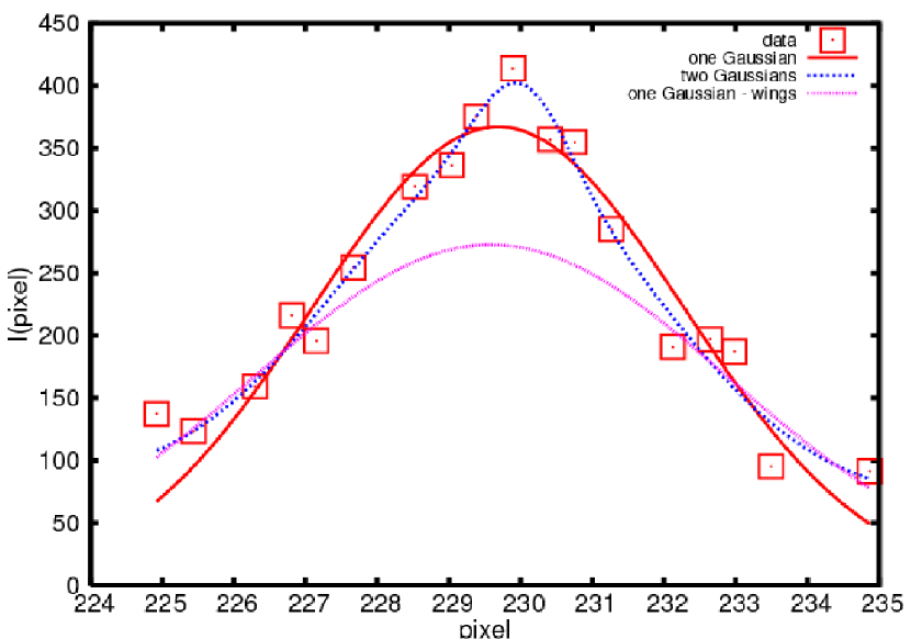
Figure 14: Median radial profile of arc A1 (square data points). Several attempts of fitting it are shown: single Gaussian (solid line), two Gaussians (long-dotted line) and single Gaussian fitting only the data points below half of the maximum of the profile (short-dotted line).

The fit improves if a combination of Gaussians are used:

$$\tilde{G}(x)=\sum_{i=1}^{M}Q_{i}\exp{-\frac{(x-\overline{x}_{i})^{2}}{2\sigma_{i}^{2}}}\;.$$ (46)

The coarsely-dotted line in Fig. 14 shows the best fit obtained by combining $M=2$ Gaussians. The reduced $\chi^{2}$ is smaller by a factor of $\sim 2$ in this case. The resulting fit consists of a combination of a broad Gaussian describing the wings of the profile, and of a narrow one describing its central part and contributing very little to the wings. This suggests that, in order to measure the width of the arc, we could use a single Gaussian to fit the external parts of the profile, without affecting significantly the measurements. For example, the Gaussian that fits only the data points below the half of the maximum of the profile is shown by the finely-dotted line. Comparing to the previously described two-Gaussian fit, the differences in the wings of the profile are minimal.

Even using multiple Gaussians, the de-convolution of the profile can be done as described above. Indeed, each Gaussian component can be de-convolved individually and summed up to provide a de-convolved profile. The arc width can be then derived straightforwardly.

The same fitting procedure can also be applied to the tangential profile of the arc, in order to correct for the PSF effects on the arc length. However, as explained above, for arcs with large length-to-width ratios, the correction is much less important than for the arc width, since the tangential profile declines much more gently than the transversal profile. For example, the best fit Gaussians describing the decline of the tangential brightness profile on both sides of arc A1 have $\sigma\gtrsim 15$ pixels. The Gaussian best fitting the wings of the radial profile shown in Fig. 14 has $\sigma=3.4$ pixels. Using Eqs. 39 and 45, the PSF correction amounts to $\sim 2\%$ for the width and to $\lesssim 0.3\%$ for the length in that example.

The width measurements made on arc A1 are displayed in Fig.13 using horizontal lines. Results are shown both for the PSF convolved and de-convolved widths. The Gaussian-equivalent width obtained by fitting the arc radial profile with a single Gaussian is $0.99"$. This is $\sim 15\%$ smaller than the Gaussian-equivalent width measured by using two Gaussians for fitting the profile ($1.14"$). The latter is very similar to the true median width ($1.15"$). Finally, the de-convolved width, obtained from the two-Gaussians fit, is $1.12"$.

The analysis made on arc A1 has been repeated over the other arc-like images in Fig. 11. We summarize the properties of all these arcs in Table 1. In column 2 we list the arc lengths (without PSF corrections), followed by several definitions of arc widths, listed in columns 3-6. We report both the maximal and the median widths and the Gaussian-equivalent widths before and after PSF-correction. In column 7, we list the arc curvature radii.

The comparison between the median and the maximal widths shows that large fluctuations of the arc thickness are possible along the azimuthal profiles. Differences of order $30\%$ are typical but the maximal width can be even $80\%$ larger than the median width, as shown for the radial arc F1 (see table). This image is located in a noisy region, near to some cluster galaxies, thus the edges of the image are very irregular. This confirms that defining the arc width - and other arc properties that depend on this definition, like the length-to-width ratio - is a critical issue.

The agreement between the Gaussian-equivalent and the median widths is generally good. The PSF-corrections are typically of order few percent, as expected given the narrow PSF of DUNE.

Some arcs are particularly straight. Two examples are the arcs D1 and F1 that have very large curvature radii. In such cases, we arbitrarily assign a curvature radius of $1000"$.

arc	$L$	$W_{\rm max}$	$W_{\rm med}$	$W_{G}$	$W_{G,0}$	$R_{c}$	$W_{0}$
A1	23.2	1.61	1.15	1.14	1.12	26.2	1.13
B1	14.3	0.98	0.81	0.81	0.77	31.5	0.7
C1	4.55	0.88	0.73	0.76	0.7	70.6	0.69
D1	3.91	0.83	0.62	0.61	0.59	1000	0.65
E1	8.04	1.17	0.93	0.94	0.86	18.5	0.73
F1	4.2	0.87	0.48	0.45	0.44	1000	0.47

Table 1: Summary of the main properties of the arcs shown in Fig. 11. Column 1: arc names. Column 2: arc lengths. Column 3-6: different definitions of arc widths (maximal, median, Gaussian-equivalent, PSF-corrected). Column 7: arc curvature radii. Column 8: arc widths in a simulation with null PSF. All quantities are given in arcsec.

By activating and/or deactivating different features of the simulator, the techniques used to analyze the images can be tested to quantify how reliable are the measurements. In the last column of Tab. 1 we show the median widths measured in a simulation where the PSF FWHM is set to zero. The remaining simulation parameters (instrument, exposure time, etc.) are not changed. Although the PSF correction is small, we notice that these newly determined widths are in a slightly better agreement with the PSF-corrected widths in column 6 (r.m.s. deviation of $\sim 0.16"$) than with the previous median or Gaussian-equivalent widths in column 4 and 5 (r.m.s. $\sim 0.23"$ and $\sim 0.25"$, respectively). This suggests that the de-convolution technique described above is correctly applied and allows to determine the true widths with an uncertainty of order one pixel.

3.5 Detectability of arcs

An important question that can be answered using our simulator is how do the properties of the arcs depend on source modeling.

First of all, we wish to determine for what intrinsic fluxes of the sources are the arcs detectable in DUNE images, assuming an exposure time of $1000$ seconds. For this purpose, we run several simulations, using the same morphological models of the sources, i.e. without changing their shapelet coefficients, their orientation and their spectral type, but changing only the input fluxes such that the apparent magnitudes in the $riz$ band vary between $m_{riz}=23$ and $m_{riz}=28$. Then, we quantify if the arcs are detectable by counting the number of pixels belonging to the arcs that emerge above a minimal S/N ratio. As done before, we fix this limit to $S/N_{\rm min}=5$.

The results of this test are shown in Fig. 15 for the arcs $A1$ to $F1$ using different line-styles. In the top-left panel, we show the arc areas above $S/N_{\rm min}$ as a function of the intrinsic apparent magnitude of the sources (in absence of lensing magnification). The limiting source magnitude for which arcs are detectable significantly differs from arc to arc, ranging between $24.5$ and $27$. The most prominent arcs, i.e. arcs A1 and B1, that are the most magnified sources, can be detected only for source intrinsic magnitudes below $25.5$ and $26$, respectively, while some shorter arcs, like arcs C1 and E1, can be detected even if the sources are fainter ($m_{riz}\lesssim 27$). We shall recall that lensing does not change the surface brightness of the sources, but only the solid angle under which they are observed. Thus, the differences between the detectability limits must reflect the different size, shape and brightness profile of the sources.

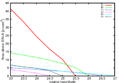
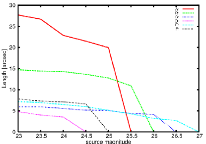
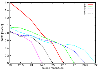
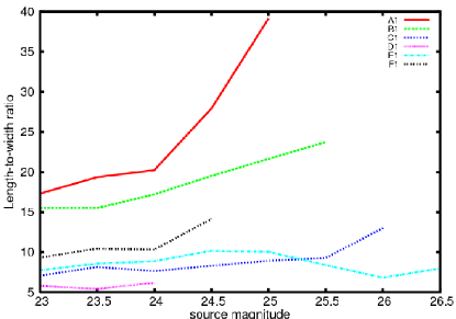
Figure 15: Arc properties as a function of the source intrinsic magnitude in the $riz$ band. Shown are the area above the minimal signal-to-noise ratio $S/N=5$ (upper-left panel), the length (upper-right panel), the width (bottom-left) and the length-to-width ratio (bottom-right panel). The different line-styles correspond to the arcs A1-F1.

The observed properties of the arcs, in particular the length and the width, obviously depend of the luminosity of the sources. In the top-right and in the bottom-left panels of Fig. 15 we show how the lengths and the widths scale as a function of the intrinsic magnitude. As expected, as the sources become fainter, the arcs shrink in both the tangential and in the radial directions. Such decrements, however, occur at different rates. While the lengths decrease slowly, the change of the arc widths is more rapid. This is clearly due to the presence of several bright knots along the azimuthal profile of the arcs (see e.g. Fig. 13). These originate from multiple images of the same source that merge from opposite sides of the critical lines. Thus, as long as the arcs emerge from the background, their length cannot become shorter than the maximal separation between the knots. Only for very faint magnitudes do the arcs break into smaller pieces and the lengths decrease rapidly. This behavior implies that the length-to-width ratio is not a constant function of the source magnitude. As shown in the bottom-right panel, especially for the longest arcs, the length-to-width ratio is generally inversely proportional to the source luminosity, once the source morphology has been fixed. For example, between $m_{riz}=23$ and $m_{riz}=25$, the length-to-width ratio of the arc A1 becomes larger by more than a factor of two. For arc B1, it grows by $\sim 65\%$ between $m_{riz}=23$ and $m_{riz}=25.5$. Also the length-to-width ratios of the arc C1 and of the radial arc F1 grow significantly.

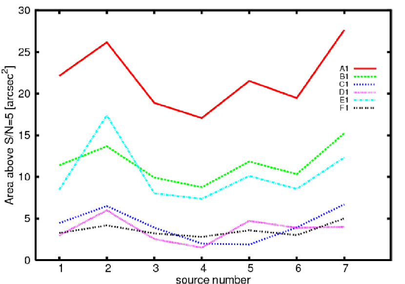
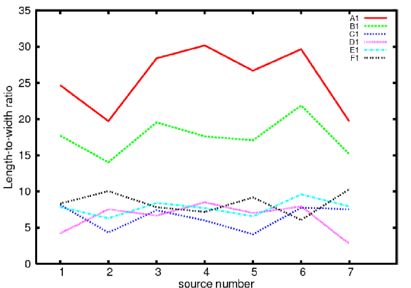
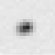
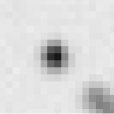
Figure 16: Top panel: Areas of the arcs A1-F1 above $S/N=5$, assuming different sets of shapelet coefficients for modeling the sources. The source models (shown in the figures below the graphs) are numbered from 1 to 7. All sources have intrinsic magnitude $m_{riz}=24$. Bottom panel: length-to-width ratio as a function of the source model

To better explain the dependence of the arc appearance on the intrinsic properties of the sources, we run new simulations, keeping the sources at the same positions but exchanging among them the sets of shapelet coefficients that determine their morphology and surface brightness distributions. In other words, we re-simulate each arc using seven different source shapes. The intrinsic magnitude of the sources was fixed to $m_{riz}=24$. This value has been chosen such that all arcs A1-F1 are detectable. In the upper graph of Fig. 16 we show the area of each arc above $S/N=5$ as a function of the source model. Each model is identified by a number running from 1 to 7. The corresponding un-lensed images of the sources are shown at the center of the frames below the graphs. Note that these are cut-outs from the left panel of Fig. 11. As anticipated earlier, by varying the morphology of the sources, different amounts of pixels belonging to the arcs surpass the detectability thresholds. In particular, the spatial extent of the arc is determined by the size of the sources, i.e. by their surface brightness. We notice that the curves corresponding to different arcs have many features in common. Indeed, they have several local minima and maxima that arise for the same source models. For example, all arcs have the largest sizes if the source model number 2 or number 7 are used, while their size is the smallest for the source model number 4. Looking at the corresponding source representations, we see that the former are low surface-brightness and spatially extended galaxies, while the latter corresponds to the most compact among the sources.

We now consider the correlation between the source model and the length-to-width ratio of their images. This is shown in the bottom graph of Fig. 16. Compared to the previous plot, we notice the opposite correlation for most of the images: for a fixed total luminosity of the sources, the most extended galaxies (the sources 2 and 7 in Fig. 16) correspond to the lowest arc length-to-width ratios.

We can interpret these results as follows. Large, low surface brightness images average magnification over a larger area. Thus, they are less distorted. Indeed, the relative changes of the lengths and of the widths of the images are caused by the convolution of the tangential and of the radial magnifications with source surface brightness distribution. The distortion effects are diluted if the source is broader. For this reason, arcs originating from compact, faint or low surface brightness sources that are barely detectable are preferentially characterized by large length-to-width ratios. These results show that comparing theory to observations, we need to know the source population the arcs are drawn. As surface brightness is unchanged, we suggest basing the detectability criterion of arcs upon it.

4 Conclusions

We presented a new code for mimicking optical observations of distant galaxies. It includes all relevant sources of noise affecting real observations, such as sky background, photon noise and effects of the atmosphere and of the instrumental PSF. The code also incorporates ray-tracing routines that allow us to include lensing effects by matter distributed between the observer and the sources.

In this work we have detailed the thorough method that we have developed in order to model the source galaxies realistically. The source morphologies are modeled via the shapelet decomposition of real galaxy images observed with HST. Four spectral templates are used to simulate the spectral energy distributions of the galaxies. Their redshift and luminosity distributions as a function of their spectral classification are derived from observed galaxy luminosity functions in the VVDS.

Being particularly suitable for simulating lensing by galaxy clusters, the code also simulates the emission from the cluster galaxy population, whose properties are obtained from semi-analytic models of galaxy formation and evolution.

Many features of the simulator have been discussed in detail. In particular, we have shown that the code can be easily used to mimic observations with a variety of existing instruments, both from the space (HST) and from the ground (LBT).

In order to illustrate the code and to introduce some potential applications, we have simulated observations of a galaxy cluster obtained from N-body simulations. These virtual observations were made using a telescope with the characteristics of the proposed space telescope DUNE.

The simulated images were analyzed using standard observational techniques. After subtracting the light of the foreground galaxies, multiple images of several distant sources that were strongly lensed by the foreground cluster can be identified. Each detected arc-like image has been classified, measuring its length, width and curvature radius.

We discussed how the properties of arcs can be measured consistently in simulations and observations, in order to facilitate the comparison with theoretical predictions. In particular, we focused on the determination of the arc widths and on how they can be corrected for the PSF broadening. For this purpose, we fit the radial profile of the arcs with multiple Gaussians. By comparing simulations with and without PSF convolution, we verified that the de-convolution technique allows one to determine the true width of the arcs with a typical error of one pixel.

By varying the characteristics of the sources, we studied the detectability limits of arcs in DUNE observations. With an exposure time of $1500$ seconds, we expect that DUNE will be able to observe arcs arising from sources whose magnitudes are fainter than $\sim 27$ in the $riz$ band. The shape of the arcs are found to be very sensitive to the properties of the sources. In particular, we found that arcs tend to acquire larger length-to-width ratios as their sources become fainter or more compact.

These results are particularly intriguing for arc statistics. Indeed, they show that observational effects may have a large impact on the abundance of arcs with large length-to width ratios, and they deserve careful investigation. We will dedicate a forthcoming paper to this subject (Meneghetti et al., in prep.). The source morphologies, and in particular sub-structures of star-forming regions, are clearly more relevant for arc statistics than is usually assumed. This is as a result of the small angular size of the bright star forming regions which are more easily distorted. Moreover, the number of very elongated images is expected to grow rapidly as a function of the depth of the observations. Thus, space missions like DUNE, capable of making deep and wide surveys thanks to their large sensitivity and field of view, are likely to discover a significant number of new gravitational arcs. The usage of efficient software for automatic arc identification (see e.g. Lenzen et al., 2005; Seidel & Bartelmann, 2007; Alard, 2006; Horesh et al., 2005; Cabanac et al., 2007) will facilitate the detection of strong lensing events in these large data sets.