Nodal domains on graphs - How to count them and why?

Abstract.

The purpose of the present manuscript is to collect known results and present some new ones relating to nodal domains on graphs, with special emphasize on nodal counts. Several methods for counting nodal domains will be presented, and their relevance as a tool in spectral analysis will be discussed.

1. Introduction

Spectral graph theory deals with the spectrum and the eigenfunctions of the Laplace operator defined on graphs. The study of the eigenfunctions, and in particular, their nodal domains is an exciting and rapidly developing research direction. It is an extension to graphs of the investigations of nodal domains on manifolds, which started already in the 19th century by the pioneering work of Chladni on the nodal structures of vibrating plates. Counting nodal domains started with Sturm’s oscillation theorem which states that a vibrating string is divided into exactly n nodal intervals by the zeros of its $\textit{n}^{th}$ vibrational mode. In an attempt to generalize Sturm’s theorem to manifolds in more than one dimension, Courant formulated his nodal domains theorem for vibrating membranes, which bounds the number of nodal domains of the $\textit{n}^{th}$ eigenfunction by n [1]. Pleijel has shown later that Courant’s bound can be realized only for finitely many eigenfunctions [2]. The study of nodal domains counts was revived after Blum et al have shown that nodal count statistics can be used as a criterion for quantum chaos [3]. A subsequent paper by Bogomolny and Schmit illuminated another fascinating connection between nodal statistics and percolation theory [4]. A recent paper by Nazarov and Sodin addresses the counting of nodal domains of eigenfunctions of the Laplacian on $\mathbb{S}^{2}$ [5]. They prove that on average, the number of nodal domains increases linearly with $n$, and the variance about the mean is bounded. At the same time, it was shown that the nodal sequence - the sequence of numbers of nodal domains ordered by the corresponding spectral parameters - stores geometrical information about the domain [6] . Moreover, there is a growing body of numerical and theoretical evidence which shows that the nodal sequence can be used to distinguish between isospectral manifolds. [7, 8].

In the present paper we shall focus on the study of nodal domains on graphs, and show to what extent it goes hand in hand or complements the corresponding results obtained for Laplacians on manifolds.

The paper is designed as follows: The next chapter summarizes some elementary definitions and background material necessary to keep this paper self contained. Next, we survey the known results regarding counting nodal domains on graphs and state a new theorem regarding the morphology of nodal domains. After these preliminaries, we present a few counting methods of nodal domains on graphs. Finally, the intimate connection between nodal sequences and isospectrality on graphs will be reviewed, and some open problems will be formulated.

2. Definitions, notations and background

A graph $\mathcal{G}=(\mathcal{V},\mathcal{B})$ is a set of vertices $\mathcal{V}=\{1,2,\ \cdots V\}$ of size $V\equiv|\mathcal{V}|$ and a set of undirected bonds (edges) $\mathcal{B}$ of size $B\equiv|\mathcal{B}|$, such that $\{i,j\}\in\mathcal{B}$ if the vertices $i$ and $j$ are connected by a bond. In this case we say that vertices $i$ and $j$ are adjacent and denote this by $i\sim j$. The degree (valency) of a vertex is the number of bonds which are connected to it. A graph is called $v$-regular if all its vertices are of degree $v$. Throughout the article, and unless otherwise stated, we deal with connected graphs with no multiple bonds or loops (a bond which connects a vertex to itself). A well known fact in graph theory is that the number of independent cycles in a graph, denoted by $r$ is equal to:

(1) $$r=B-V+Co$$

where $Co$ is the number of connected components in $\mathcal{G}$. We note that $r$ is also the rank of the fundamental group of the graph. A tree is a graph for which $r=0$.
Let $g$ be a subgraph of $\mathcal{G}$. We define the interior of $g$ as the set of vertices whose adjacent vertices are also in $g$. The boundary of $g$ is the set of vertices in $g$ which are not in its interior.

A graph $\mathcal{G}$ is said to be properly colored if each vertex is colored so that adjacent vertices have different colors. $\mathcal{G}$ is k-colorable if it can be properly colored using k colors. The chromatic number $\chi(\mathcal{G})$ is k if $\mathcal{G}$ is k-colorable and not (k-1)-colorable. A very simple observation, which we will use later, is that $\chi(\mathcal{G})\leq V$.

$\mathcal{G}$ is called bipartite if its chromatic number is 1 or 2. However, since a chromatic number 1 corresponds to a graph with no bonds, and we are dealing only with connected graphs, we can exclude this trivial case and say that for a bipartite graph, $\chi=2$. The vertex set of a bipartite graph $\mathcal{G}$ can be partitioned into two disjoint sets, say $\mathcal{V}_{1}$ and $\mathcal{V}_{2}$, in such a way that every bond of $\mathcal{G}$ connects a vertex from $\mathcal{V}_{1}$ with a vertex from $\mathcal{V}_{2}$. We then have the following notation: $\mathcal{G}=(\mathcal{V}_{1}\cup\mathcal{V}_{2},\mathcal{B})$ [20].

The adjacency (connectivity) matrix of $\mathcal{G}$ is the symmetric $V\times V$ matrix $C=C(\mathcal{G})$ whose entries are given by:

$$C_{ij}=\left\{\begin{array}[]{ll}1,&\textrm{if $i$ and $j$ are adjacent}\\ 0,&\textrm{otherwise}\end{array}\right.$$

Laplacians on graphs can be defined in various ways. The most elementary way relies only on the topology (connectivity) of the graph, and the resulting Laplacian is an operator on a discrete and finite-dimensional Hilbert space. These operators or their generalizations to be introduced below will be referred to as “discrete” or “combinatorial” Laplacians. One can construct the Laplacian operator as a differential operator if the bonds are endowed with a metric, and appropriate boundary conditions are required at the vertices. The resulting operator should be referred to as the “metric” Laplacian. However, because the metric Laplacian is identical with the free Schrödinger operator (i.e. with no potential) on the graph, one often refers to this system as a “Quantum Graph” - a misnomer which is now hard to eradicate. In the sequel we shall properly define and discuss the relevant versions of Laplacians on graphs.

The discrete Laplacian, of $\mathcal{G}$, is the matrix

(2) $$L(\mathcal{G})=D-C\ ,$$

where $D$ is the diagonal matrix whose $i^{th}$ diagonal entry is the degree of the vertex $i$, and $C$ is the adjacency matrix of $\mathcal{G}$. A generalized Laplacian, $L^{{}^{\prime}}$ is a symmetric $V\times V$ matrix with off-diagonal elements defined by: $L^{{}^{\prime}}_{ij}<0$ if vertices $i$ and $j$ are adjacent, and $L^{{}^{\prime}}_{ij}=0$ otherwise. There are no constraints on the diagonal elements of $L^{{}^{\prime}}$.

The eigenvalues of $L(\mathcal{G})$ together with their multiplicities, are known as the spectrum of $\mathcal{G}$. To each eigenvalue corresponds (at least one) eigenvector whose entries are labeled by the vertices indexes. It is well known that the eigenvalues of the combinatorial Laplacian are non-negative. Zero is always an eigenvalue and its multiplicity is equal to the number of connected components of $\mathcal{G}$. An important property regarding spectra of large $v$-regular graphs is that the limiting spectral distribution is symmetric about $\lambda=v$, and is supported on the interval $[v-2\sqrt{v-1},v+2\sqrt{v-1}]$ [18].

An extensive survey of the spectral theory of discrete Laplacians can be found in [21, 22, 23].

To define quantum graphs a metric is associated to $\mathcal{G}$. That is, each bond is assigned a positive length: $L_{b}\in(0,\infty)$. The coordinate along the bond $b$ is denoted by $x_{b}$. The total length of the graph will be denoted by $\mathcal{L}=\sum_{b\in\mathcal{B}}L_{b}$. This enables to define the metric Laplacian (or free Schrödinger operator) on the graph as the negative second derivative $-\frac{{\rm d}^{2}\ }{{\rm d}x^{2}}$ on each bond. The domain of this operator on the graph is the space of functions which connect continuously across vertices and which belong to the Sobolev space $W^{2,2}(b)$ on each bond b. Moreover, vertex boundary conditions are imposed to render the operator self adjoint. We shall consider in this paper the Neumann and Dirichlet boundary conditions:

(3) $${\rm Neumann\ condition\ on\ the\ vertex\ }i:\ \ \ \ \ \sum_{b\in S^{(i)}}\left.\frac{{\rm d}\ \ \ }{{\rm d}x_{b}}\ \psi_{b}(x_{b})\right|_{x_{b}=0}\ =\ 0\ \ ,$$

(4) $${\rm Dirichlet\ condition\ on\ the\ vertex\ }i:\ \ \ \ \ \ \ \ \ \ \ \left.\psi_{b}(x_{b})\right|_{x_{b}=0}=0\ ,$$

where $S^{(i)}$ denotes the group of bonds which emerge from the vertex $i$ and the derivatives in (3) are directed out of the vertex $i$. The eigenfunctions are the solutions of the bond Schrödinger equations:

(5) $$\ \ \forall b\in\mathcal{B}\ \ -\frac{{\rm d}^{2}\ }{{\rm d}x^{2}}\psi_{b}=k^{2}\psi_{b},$$

which agree on the vertices and satisfy at each vertex boundary conditions of the type (3) or (4). The spectrum $\{k_{n}^{2}\}_{n=1}^{\infty}$ is discrete, non-negative and unbounded. One can generalize the metric Laplacian by including potential and magnetic flux that are defined on the bonds. Other forms of boundary conditions can also be used. However, these generalizations will not be addressed here, and the interested reader is referred to two recent reviews [13, 14].

Finally, two graphs, $\mathcal{G}$ and $\mathcal{H}$, are said to be isospectral if they posses the same spectrum (same eigenvalues with the same multiplicities). This definition holds both for discrete and quantum graphs.

3. Nodal domains on graphs

Nodal domains on graphs are defined differently for discrete and metric graphs.
$\bullet\$Discrete graphs: Let $\mathcal{G}=(\mathcal{V},\mathcal{B})$ be a graph and let $\bf f$=$(f_{1},f_{2},\ldots,f_{V})$ be a real vector. We associate the real numbers $f_{i}$ to the vertices of $\mathcal{G}$ with $i=1,2,\ldots,V$. A nodal domain is a maximally connected subgraph of $\mathcal{G}$ such that all vertices have the same sign with respect to $\bf f$. The number of nodal domains with respect to a vector $\bf f$ is called a nodal domains count, and will be denoted by $\nu(\bf f)$. The maximal number of nodal domains which can be achieved by a graph $\mathcal{G}$ will be denoted by $\nu_{\mathcal{G}}$. The nodal sequence of a graph is the number of nodal domains of eigenvectors of the Laplacian, arranged by increasing eigenvalues. This sequence will be denoted by $\{\nu_{n}\}_{n=1}^{V}$.

The definition of nodal domains should be sharpened if we allow zero entries in $\bf f$. Two definitions are then natural:

• A strong positive (negative) nodal domain is a maximally connected subgraph $\mathcal{H}$ of $\mathcal{G}$ such that $\textit{f}_{i}>0$ ($\textit{f}_{i}<0$) for all $i\in\mathcal{H}$.

• A weak positive (negative) nodal domain is a maximally connected subgraph $\mathcal{H}$ of $\mathcal{G}$ such that $\textit{f}_{i}\geq 0$ ($\textit{f}_{i}\leq 0$) for all $i\in\mathcal{H}$.

In both cases, a positive (negative) nodal domain must consist of at least one positive (negative) vertex. According to these definitions, it is clear that the weak nodal domains count is always smaller or equal to the strong one.
$\bullet\$Metric graphs: Nodal domains are connected domains of the metric graph where the eigenfunction has a constant sign. The nodal domains of the eigenfunctions are of two types. The ones that are confined to a single bond are rather trivial. Their length is exactly half a wavelength and their number is on average $\frac{k\mathcal{L}}{\pi}$. The nodal domains which extend over several bonds emanating from a single vertex vary in length and their existence is the reason why counting nodal domains on graphs is not a trivial task. The number of nodal domains of a certain eigenfunction on a general graph can be written as

(6) $$\mu_{n}=\frac{1}{2}\sum_{i}\sum_{b\in S^{(i)}}\left\{\left\lfloor\frac{k_{n}L_{b}}{\pi}\right\rfloor+\frac{1}{2}\left(1-(-1)^{\lfloor\frac{k_{n}L_{b}}{\pi}\rfloor}\mathrm{sign}[\phi_{i}]\mathrm{sign}[\phi_{j}]\right)\right\}-B+V\$$

where $\lfloor x\rfloor$ stands for the largest integer which is smaller than $x$, and $\phi_{i},\phi_{j}$ are the values of the eigenfunction at the vertices connected by the bond $b=\{i,j\}$ [17]. (6) holds for the case of an eigenfunction which does not vanish on any vertex: $\forall i\,\,\,\phi_{i}\neq 0$, and there is no cycle of the graph on which the eigenfunction has a constant sign. The last requirement is true for high enough eigenvalues where half the wavelength is smaller than the length of the shortest bond. This restriction, which is important for low eigenvalues, was not stated in [17].

Nodal domains on quantum graphs can be also defined and counted in an alternative way. Given an eigenfunction, we can associate to it the vector ${\bm{\phi}}=(\phi_{1},\ldots,\phi_{V})$ of its values on the vertices and count the nodal domains of this vector as in the case of a discrete graph, explained above. The reasoning behind this way of counting is that the values of the eigenfunction on the vertices $\{\phi_{i}\}_{i=1}^{V}$ together with the eigenvalue $k^{2}$ store the complete information about the values of the eigenfunction everywhere on the graph. We thus have two independent ways to define and count nodal domains on metric graphs. To distinguish between them we shall refer to the first as metric nodal domains, and the number of metric domains in the $n^{th}$ eigenfunction will be denoted by $\mu_{n}$. The domains defined in terms of the values of the eigenfunction on the vertices will be referred to as the discrete nodal domains. The number of the discrete nodal domains in the $n^{th}$ eigenfunction will be denoted by $\nu_{n}$, similar to the notation of this count for the discrete graphs.

As far as counting nodal domains is concerned, trees behave as one dimensional manifolds, and the analogue of Sturm’s oscillation theory applies for the eigenfunctions of the discrete [9] and the metric Laplacians [10, 11, 12, 15], as long as the eigenvector (or the eigenfunction) does not vanish at any vertex. Thus we have $\nu_{n}=n$ for discrete tree graphs and $\mu_{n}=n$ for metric ones.

Similarly, Courant’s theorem applies for the eigenfunctions of both the discrete and the metric versions of the Laplacian on any graph: $\nu_{n}\leq n$,   $\mu_{n}\leq n$, [16, 17]. It should be noted that there is a correction due to multiplicity of the $n^{th}$ eigenvalue and the upper bound becomes $n+m-1$, where $m$ is the multiplicity [16]. However, sharper lower and upper bounds for the number of nodal domains were discovered recently. Berkolaiko provided a lower bound for the nodal domains count for both the discrete and the metric cases [27]. He showed that the nodal domains count of the $n^{th}$ eigenfunction of the Laplacian (either discrete or metric) has no less than $n-r$ nodal domains ($r$ is the number of independent cycles in the graph). Again, this is valid if the eigenfunction has no zero entries and it belongs to a simple eigenvalue. When $n-r<0$, this result is trivial since a nodal domains count is positive by definition. We note that for metric graphs this theorem does not hold when the discrete count is used. This can be explained by the simple observation that $n-r$ grows unbounded while the discrete count is bounded by the number of vertices.

A global upper bound for the nodal domains count of a graph $\mathcal{G}$ was derived in [28]: The maximal number of nodal domains on $\mathcal{G}$ was proven to be smaller or equal to $\nu_{\mathcal{G}}V-\chi+2$, where $\chi$ is the chromatic number of $\mathcal{G}$. This bound is valid for any vector, not only for Laplacian eigenvectors.

To end this section we shall formulate and prove a few results which show that not all possible subgraphs can be nodal domains of eigenvectors of the discrete Laplacians of $v$-regular graphs. The topology and connectivity of nodal domains are restricted, and the restrictions depend on whether the eigenvalue is larger or smaller than the spectral mid-point $v$.

Theorem 3.1.

Let $\mathcal{G}$ be a $v$-regular graph. Then the following statements hold:

i. For all eigenvectors with eigenvalue $\lambda>v$ the nodal domains do not have interior vertices.

ii. For all eigenvectors with eigenvalue $\lambda<v$, all the nodal domains consist of at least two vertices.

iii. For all eigenvectors with eigenvalue $\lambda<v-k$ (and $k<v$), in every nodal domain there exists at least one vertex with a degree (valency) which is larger than $k$.

Proof.

Let $\bf{f}$ be an eigenvector with no zero entries of the discrete Laplacian, corresponding to an eigenvalue $\lambda$. Let $g$ be a nodal domain of $\mathrm{\bf{f}}$.

i. Assume that $i$ is an interior vertex in $g$. Hence, the signs of $f_{j}$ for all $j\sim i$ are the same as the sign of $f_{i}$. This is not compatible with

(7) $$-\sum_{j\sim i}f_{j}=(\lambda-v)f_{i}$$

for $\lambda>v$. Hence $g$ cannot have any interior vertices.

ii. Assume that the subgraph $g$ consists of a single vertex $i$. Thus on all its neighbors $j\sim i$, the sign of $f_{j}$ is different from the sign of $f_{i}$. This is not compatible with

(8) $$-\sum_{j\sim i}f_{j}=-(v-\lambda)f_{i}$$

for $\lambda<v$. Hence $g$ cannot consist of a single vertex.

iii. Denote the complement of the nodal domain (subgraph) $g$ in $\mathcal{V}$ by $g^{c}$. For all the vertices $i$ in $g$

(9) $$(L\textbf{f})_{i}\ =\ vf_{i}-\sum_{j\in g}C_{j,i}f_{j}-\sum_{l\in g^{c}}C_{l,i}f_{l}\ =\ \lambda f_{i}\ .$$

Summing over $i\in g$ we get:

(10) $$(v-\lambda)\sum_{i\in g}f_{i}=\sum_{i\in g}\left(\sum_{j\in g}C_{j,i}f_{j}+\sum_{l\in g^{c}}C_{l,i}f_{l}\right)$$

Assuming for convenience that $f_{i}$ are positive for $i\in g$, the rightmost sum in the equation above is non positive, and therefore

(11) $$(v-\lambda)\sum_{i\in g}f_{i}\ \leq\ \sum_{i\in g}\sum_{j\in g}C_{j,i}f_{j}=\sum_{i\in g}v_{i}f_{i}\ \leq\ \hat{v}\sum_{i\in g}f_{i}\ .$$

Here, $v_{i}=\sum_{j\in g}C_{j,i}$ is the valency (degree) of the $i^{th}$ vertex in $g$, and $\hat{v}$ denotes the largest valency in the subgraph. Since it is assumed that $\lambda<v-k$ we get

(12) $$k\ <\ \hat{v}\ ,$$

which completes the proof. ∎

This theorem holds also for an eigenvector $\bf{f}$ which has zero elements with the only exception being the failure of part i when using the weak count. The case $\lambda=v$ deserves special attention. As long as the nodal domain under study has no vanishing entries, it cannot consist of a single vertex nor can it have interior vertices. Namely, for $\lambda=v$, statements i and ii of Theorem 3.1. are valid simultaneously. Otherwise, one should treat separately the strong and the weak counts. For the strong count, and $\lambda=v$ a nodal domain cannot have an interior vertex. However, using the weak count for $\lambda=v$ one finds that no single vertex domains can exists, as in Theorem 3.1.ii.

Item iii of Theorem 3.1 can be used to provide a $\lambda$ dependent bound on the number of nodal domains of eigenvectors corresponding to eigenvalues $\lambda<v$. Define the integer $k$ as $k=v-\lceil\lambda\rceil$. Theorem 3.1.iii implies that every nodal domain occupies at least $k+2$ vertices. Thus, their number is bounded by $\frac{V}{k+2}$. Courant theorem guarantees that the number of nodal domains is bounded by the spectral count $\mathcal{N}(\lambda)$. This information together with the known expression for the expectation value of $\mathcal{N}(\lambda)$ over the ensemble of random graphs, enable us to show that for large $v$ and $V$, the bound $\frac{V}{k+2}$ is more restrictive than the Courant bound. Unlike Pleijel’s result, this bound is not uniform for the entire spectrum, and it applies only to the lower half of the eigenvalues with $\lambda<v$.

Theorem 3.1 can be easily extended to the nodal properties of the eigenvectors of the generalized Laplacian, provided that the weights at each vertex sum up to a constant $v$ which is the same for the entire graph.

4. How to count nodal domains on graphs?

When discussing nodal domains counting, we must make a clear distinction between algorithmic and analytic methods. In the first class, we include computer algorithms. They vary in efficiency and reliability, but they have one feature in common, namely, that the number of nodal domains is provided not as a result of a computation, but rather, it follows from a systematic counting process. The most widely used method is the Hoshen-Kopelman algorithm (HK) for counting nodal domains on 2-dimensional domains [30]. Analytic methods provide the number of nodal domains as a functional of the function and the domain under study. The functional might be quite complicated, and not efficient when implemented numerically. An example of an analytical method for nodal domains counting in one dimension, is given by

(13) $$\nu=\int_{a}^{b}\delta\left(f(x)\right)\left|\frac{{\rm d}f(x)}{{\rm d}x}\right|{\rm d}x\ +\ 1\ ,$$

where the nodal domains of $f(x)$, in the interval $[a,b]$ are provided (assuming that $f(a)f(b)\neq 0$). While counting in 1-d is simple, there is no analytic counting method for computing the number of nodal domains in higher dimensions: the complicated connectivity allowed in high dimensions renders the counting operation too non local.

Graphs, which are in some sense intermediate between one and two dimensions still allow several analytic counting methods which we discuss here. An example of an analytical count is given by (6). The HK algorithm is well suited for graphs which are grids. However, it is not as efficient when the graph under study is highly irregular. Although the HK algorithm fails for very complex graphs, other algorithms, called labeling algorithms, display linear efficiency ([46],[47]).
Method III. in the following list, in addition of providing an analytical expression for the nodal domain count, can also be implemented as a computer algorithm. We show that it performs as efficiently as the labeling algorithm.

The counting methods that we present here are aimed for the discrete counting of both discrete and metric graphs. In what follows, we assume that a vector $\bf f$ is associated to the vertex set with entries $f_{i}$. The nodal domains are defined with respect to $\bf f$.

4.1. Method I. - Counting nodal domains in terms of flips

We define a flip as a bond on the graph which connects vertices of opposite signs with respect to a vector $\bf f$. The sign vector of $\bf f$, denoted by $\widetilde{\bf f}$, is defined by $\widetilde{f}_{i}\equiv\textrm{sign}(f_{i})$. For the time being, it is assumed that $\bf f$ has no zero entries. The general situation will be discussed later. We denote the set of flips on the graph by $\mathcal{F}(\bf f)$:

(14) $$\mathcal{F}(\textbf{f})=\{(u,v)\in\mathcal{B}\mid f_{v}f_{u}<0\}\ .$$

The cardinality of $\mathcal{F}(\bf f)$ will be denoted by $\mathrm{F}(\bf f)$.

Lemma 4.1.

The number of flips of a sign vector $\widetilde{\bf f}$, can be expressed as

(15) $$\mathrm{F}(\bf{f})=\mathrm{F}(\widetilde{\bf f})=\frac{1}{4}(\widetilde{\bf f},L\widetilde{\bf f})\ .$$

Proof.

Using:

(16) $$(\widetilde{\bf f},L\widetilde{\bf f}) = \frac{1}{2}\sum_{v\sim u}(\widetilde{f}_{v}-\widetilde{f}_{u})^{2}$$

(19) $$(\widetilde{f}_{v}-\widetilde{f}_{u})^{2} = \left\{\begin{array}[]{ll}4,&\textrm{if $\widetilde{f}_{v}$ and $\widetilde{f}_{u}$ have opposite signs}\\ 0,&\textrm{if $\widetilde{f}_{v}$ and $\widetilde{f}_{u}$ have the same sign}\end{array}\right.$$

∎

Using the number of flips, one can get an expression for the number of nodal domains:

Theorem 4.2.

Given a connected graph $\mathcal{G}$ on $V$ vertices, $B$ bonds (and $r$ cycles) and a vector $\bf f$, then the number of nodal domains of $\bf f$ is:

(20) $$\nu(\mathrm{\bf{f}})=\frac{1}{4}(\widetilde{\bf f},L\widetilde{\bf f})+V-B+l(\mathrm{\bf{f}})=\frac{1}{4}(\widetilde{\bf f},L\widetilde{\bf f})-(r-l(\mathrm{\bf{f}}))+1$$

where $l(\bf{f})$ is the number of independent cycles in $\mathcal{G}$ of constant sign (with respect to $\bf f$). The second equality above is based on equation (1).

Proof.

Let us remove all the flips from the graph. We are now left with a possibly disconnected graph $\widetilde{\mathcal{G}}$. There is a bijective mapping between components of $\widetilde{\mathcal{G}}$ and nodal domains of $\mathcal{G}$. Hence, the number of components in $\widetilde{\mathcal{G}}$ is equal to the nodal domains count of $\mathcal{G}$ with respect to $\bf f$. Let the number of nodal domains in $\mathcal{G}$ be denoted by $\nu(\bf f)$. Using (1), it is clear that for the $i^{th}$ component (where $i=1,2,\ldots,\nu(\bf{f})$): $r_{i}=B_{i}-V_{i}+1$ where $r_{i}$, $B_{i}$ and $V_{i}$ are the number of cycles, bonds and vertices of the $i^{th}$ component, respectively. It is also clear that all the cycles in $\widetilde{\mathcal{G}}$ are of constant sign, since there are no flips in $\widetilde{\mathcal{G}}$. Thus, by our notation $r_{i}=l_{i}$. Let us sum over the components:

(21) $$l(\mathrm{\bf{f}})=\sum_{i=1}^{\nu}l_{i}=\sum_{i=1}^{\nu}(B_{i}-V_{i}+1)=(B-\mathrm{F}(\textbf{f}))-V+\nu(\bf{f})$$

Combining (15) with (21), we get (20). ∎

(20) is valid only for vectors $\bf f$ with no zero entries. In order to be able to handle a zero entry in $\bf f$, we must perform a transformation on the graph. For a strong nodal count, we simply delete all the zero vertices along with the bonds connected to them from the graph, and then apply (20) on the new graph (with the new Laplacian). For a weak nodal count we replace each zero vertex by two vertices, one positive and one negative (not connected to each other), and connect them to all vertices which were connected to the original one. Now we can apply (20), and get the desired result. Notice that this correction fails in the case of a zero vertex whose neighbors are of the same sign (in this case an artificial nodal domain is added). However, the situation above can not occur for an eigenvector of a discrete Laplacian. This way of handling zero entries can be adapted for the following counting methods as well and will not be repeated in the sequel.

Using (20), we can write some immediate consequences:

(22) $$\mathrm{F}(\textbf{f}_{n})+1-r\leq\nu_{n}\leq\mathrm{F}(\textbf{f}_{n})+1$$

(23) $$n-r-1\leq\mathrm{F}(\textbf{f}_{n})\leq n+r-1$$

(22) results from the obvious fact that $0\leq l\leq r$, while (23) is a consequence of Courant’s nodal domains theorem and Berkolaiko’s theorem which states that $n-r\leq\nu_{n}$.
In order to make use of (20), one must compute $l(\bf{f})$ which is not given explicitly in terms of f. Thus, it cannot be considered as an analytic counting method, nor does it offer computational advantage (There is no known efficient algorithm which counts all the cycles of constant sign with respect to f). However, it offers a useful analytical tool for deriving other results, and it makes a useful connection between various quantities defined on the graph.

4.2. Method II. – Partition function approach

Foltin derived a partition function approach to counting nodal domains of real functions in two dimensions [32]. It can be adapted for graphs in the following way: Each vertex, $i$, is assigned an auxiliary “spin” variable $s_{i}$ where $s_{i}=\pm 1$ (a so called Ising-spin). Thus, given a certain function $\bf{f}$ on the graph, each vertex is assigned with two “spins” $s_{i}$ and $\widetilde{f}_{i}$. Let $\bf s$ denote the auxiliary spin vector: $\textbf{s}=(s_{1},s_{2},\ldots,s_{V})$. Foltin introduced a weight to each configuration of the spins model. It assigns the value $1$ to configurations in which all spins $s_{i}$ belonging to the same nodal domain (with respect to $\bf{f}$) are parallel, while spins of different domains might have different values. The weight reads:

(24) $$w(\textbf{f},\textbf{s})=\prod_{i,j:\ C_{i,j}=1}\left[1-\frac{1+\widetilde{f}_{i}\widetilde{f}_{j}}{2}\cdot\frac{1-s_{i}s_{j}}{2}\right]\ .$$

It can be easily checked that this form satisfies the requirements stated above: The weight can take the values one or zero. It is one if and only if each factor in the product is equal to one. A certain factor is one, in either one of the two cases: if $\widetilde{f}_{i}\neq\widetilde{f}_{j}$ ($i,j$ belong to different domains) - this allows the Ising-spins in different domains to be independent of each other. The second case is if $i,j$ are in the same domain, $\widetilde{f}_{i}=\widetilde{f}_{j}$ and the corresponding Ising-spins are equal, $s_{i}=s_{j}$. Let us now sum over all possible spin configurations $\{s_{i}\}$ to get the partition function

(25) $$Z(\textbf{f})\equiv\sum_{\{\textbf{s}\}}w(\textbf{f},\textbf{s})\ .$$

For the configurations whose weight has the value one, the spins have equal signs over each nodal domain and different domains are independent of each other. Hence, the total number of such configurations is:

(26) $$Z(\textbf{f})=2^{\nu(\textbf{f})}\ ,$$

where $\nu(\textbf{f})$ is the number of nodal domains of the vector f. The nodal domains count is:

(27) $$\nu(\mathrm{\bf{f}})=\frac{1}{\ln 2}\ln Z(\textbf{f})\approx 1.44\ln Z(\textbf{f}).$$

The partition function approach provides an explicit formula for the number of nodal domains, and therefore it belongs to the analytic and not to the algorithmic counting methods. As a matter of fact, it is highly inefficient for practical computations. It involves running over all possible spin configurations $\{s_{i}\}$, where $s_{i}=\pm 1$. There are $2^{V}$ different configurations, and as $V$ increases the efficiency deteriorates rapidly.

The partition function approach can be used as a basis for the derivation of some identities involving the graph and a vector $\bf f$ defined on it. It is convenient to introduce the following notations:

$$b\equiv\{i,j\}$$

$$\varphi_{b}\equiv\frac{1+\widetilde{f}_{i}\widetilde{f}_{j}}{2}$$

$$\sigma_{b}\equiv\frac{1-s_{i}s_{j}}{2}$$

Where $\widetilde{\bf f}$ and $\bf s$ are as before, and $b$ is an undirected bond. We generalize the partition function by introducing a new parameter $x$ into the definitions

(28) $$w(\textbf{f},\textbf{s};x) = \prod_{b\in\mathcal{B}}[1-\varphi_{b}\sigma_{b}x]$$

(29) $$Z(\textbf{f};x) \equiv \sum_{\{\textbf{s}\}}w(\textbf{f},\textbf{s};x)=\sum_{\{\textbf{s}\}}\prod_{b\in\mathcal{B}}(1-\varphi_{b}\sigma_{b}x)$$

(30) $$Z(\textbf{f};1) = 2^{\nu(\textbf{f})}$$

where $x$ can assume any real or complex value. At $x=1$, the generalized partition function is identical to (25).

Let us now perform the summation over all the vectors s, and compute the coefficient of $x^{k}$. To get all the contributing terms we have to sum over all choices of $k$ brackets from (29), in which $x$ appears. Non vanishing contributions occur whenever both $\varphi_{b}$ and $\sigma_{b}$ are equal to one. Since we are only summing over s, we only need to check when $\sigma_{b}=1$. This happens if and only if the s vector has a flip on the bond $b$. Since we choose $k$ brackets (which is equivalent to choosing $k$ bonds), we need to count how many s vectors have flips on all these $k$ bonds. The signs of those s vectors on bonds which are not contained in this choice of $k$ bonds are irrelevant. If we observe the choice of $k$ bonds $(b_{1},\ldots,b_{k})$, we notice that each connected component, within this choice, contributes a factor of 2, since the symmetry of turning each plus to minus and vice versa, does not change the flip properties. Using (1) we see that the number of connected components with respect to the choice of $k$ bonds is: $Co(b_{1},\ldots,b_{k})=V-k+r(b_{1},\ldots,b_{k})$, where $r(b_{1},\ldots,b_{k})$ is the number of independent cycles that are contained in this choice. Finally we notice that a cycle of odd length cannot have flips on all of its bonds, so we will not sum over choices of $b_{1},\ldots,b_{k}$ which contain a cycle of odd length. Thus, the sum over s yields:

(31) $$Z(\textbf{f};x) = \sum_{k=0}^{B}\ \ \sideset{}{{}^{\prime}}{\sum}_{b_{1},\ldots,b_{k}\in\mathcal{B}}\ \ \prod_{i=1}^{k}(\varphi_{b_{i}})2^{V-k+r(b_{1},\ldots,b_{k})}(-1)^{k}x^{k}$$

$$= {}2^{V}\sum_{k=0}^{B}\frac{(-1)^{k}}{2^{k}}\left[\sideset{}{{}^{\prime}}{\sum}_{b_{1},\ldots,b_{k}\in\mathcal{B}}\ \ \prod_{i=1}^{k}(\varphi_{b_{i}})2^{r(b_{1},\ldots,b_{k})}\right]x^{k}$$

Where $\sideset{}{{}^{\prime}}{\sum}_{b_{1},\ldots,b_{k}\in\mathcal{B}}$ stands for summation on all the possibilities to choose k bonds $b_{1},\ldots,b_{k}\in\mathcal{B}$ such that the subgraph they form do not contain an odd cycle. We can now derive some immediate properties of the generalized partition function. To start, we compute the leading four derivatives at $x=0$ to demonstrate the counting techniques involved. Some more effort is required to compute the higher derivatives.

(32) $$\hskip 28.45274ptZ(\textbf{f};0) = \ 2^{V}$$

(33) $$\hskip 28.45274ptZ^{(1)}(\textbf{f};0) = -2^{V-1}\sideset{}{{}^{\prime}}{\sum}_{b\in\mathcal{B}}\varphi_{b}=-2^{V-1}(B-\mathrm{F}(\bf{f}))$$

(34) $$Z^{(2)}(\textbf{f};0) = \ 2!\ 2^{V-2}\sideset{}{{}^{\prime}}{\sum}_{b_{1},b_{2}\in\mathcal{B}}\ \prod_{i=1}^{2}(\varphi_{b_{i}})=2^{V-1}{B-\mathrm{F}(\bf{f})\choose 2}$$

(35) $$Z^{(3)}(\textbf{f};0) = -3!\ 2^{V-3}\sideset{}{{}^{\prime}}{\sum}_{b_{1},\ldots,b_{3}\in\mathcal{B}}\ \prod_{i=1}^{3}(\varphi_{b_{i}})=-3!\ 2^{V-3}\left[{B-\mathrm{F}(\bf{f})\choose 3}-C_{3}\right]$$

(36) $$Z^{(4)}(\textbf{f};0) = \ 4!\ 2^{V-4}\sideset{}{{}^{\prime}}{\sum}_{b_{1},\ldots,b_{4}\in\mathcal{B}}\ \prod_{i=1}^{4}(\varphi_{b_{i}})$$

$$= 4!\ 2^{V-4}\left\{2C_{4}+\left[{B-\mathrm{F}(\bf{f})\choose 4}-C_{4}-\widetilde{C}_{3}\right]\right\}$$

$$= 4!\ 2^{V-4}\left[{B-\mathrm{F}(\bf{f})\choose 4}+C_{4}-\widetilde{C}_{3}\right]$$

Where $C_{3}$ is the number of triangles of constant sign, $C_{4}$ is the number of cycles of length 4 of constant sign, and $\widetilde{C}_{3}=C_{3}(B-\mathrm{F}(\textbf{f})-3)$ is the number of choices of 4 non-flips bonds which contain a triangle. In the evaluation of the function and its first three derivatives we have used the identity $\forall n\leq 3\ \ r(b_{1},\ldots,b_{n})=0$ when $b_{1},\ldots,b_{n}$ contain no odd cycles.

The partition function is a polynomial of degree less than or equal to the number of bonds. For a graph $\mathcal{G}$ with $B$ bonds and $Co$ connected components, the polynomial is of degree $B$ if and only if $\mathcal{G}$ is bipartite and the function $\bf f$ is of constant sign on each connected component. This follows from two observations: first, a well known theorem in graph theory states that a graph $\mathcal{G}$ is bipartite if and only if it contains no cycles of odd length. Thus we can choose all the bonds in $\mathcal{G}$ without having an odd cycle contained in this choice. Second, unless $\bf f$ is of constant sign on each connected component, we will encounter a flip and hence the multiplication over all $\varphi_{b_{i}}$ will vanish. If $\mathcal{G}$ is bipartite, the coefficient of $x^{B}$ is $2^{Co}$.

While the value of the polynomial at $x=1$ has an immediate application through (30), we can evaluate it for other values. Let us choose $\bf f$ to be a vector of constant sign. This way $\varphi_{b_{i}}=1$ for all $i=1,2,\ldots,B$. Hence (31) reduces to:

(37) $$2^{V}\sum_{k=0}^{B}\frac{(-1)^{k}}{2^{k}}\left(\sideset{}{{}^{\prime}}{\sum}_{b_{1},\ldots,b_{k}\in\mathcal{B}}2^{r(b_{1},\ldots,b_{k})}\right)x^{k}.$$

On the other hand, (29) equals:

(38) $$\sum_{\{\textbf{s}\}}\prod_{b\in\mathcal{B}}(1-\sigma_{b}x).$$

Choosing $x=-n+1$ where $n\in\mathbb{Z}$ and using the fact that (37) and (38) are equal, we get:

(39) $$\frac{1}{2^{V}}\sum_{\{\textbf{s}\}}n^{\mathrm{F}(\bf s)}=\sum_{k=0}^{B}\frac{(-1)^{k}}{2^{k}}\left(\sideset{}{{}^{\prime}}{\sum}_{b_{1},\ldots,b_{k}\in\mathcal{B}}2^{r(b_{1},\ldots,b_{k})}\right)(-n+1)^{k}.$$

For random vectors $\bf s$, uniformly distributed, the left hand side can be interpreted as the average over this ensemble of the quantity: $n^{\mathrm{F}(\bf s)}$. Let us choose two special values for n. If we choose $n=-1$, the left hand side is just the difference between the probability that a random vector $\bf s$ on the graph has an even number of flips, and an odd number of flips. The right hand side is:

(40) $$\sum_{k=0}^{B}(-1)^{k}\sideset{}{{}^{\prime}}{\sum}_{b_{1},\ldots,b_{k}\in\mathcal{B}}2^{r(b_{1},\ldots,b_{k})}.$$

For $n=2$, we get:

(41) $$\frac{1}{2^{V}}\sum_{\{\textbf{s}\}}2^{\mathrm{F}(\textbf{s})}=\sum_{k=0}^{B}\frac{1}{2^{k}}\sideset{}{{}^{\prime}}{\sum}_{b_{1},\ldots,b_{k}\in\mathcal{B}}2^{r(b_{1},\ldots,b_{k})}.$$

An example of the use of the polynomial could be in proving that on a tree, the probability of an even number of flips is equal to the probability of an odd number of flips. We use Eq. (40) and see that this difference of probabilities is equal to: $\sum_{k=0}^{B}(-1)^{k}{B\choose k}=0$.
Other possible identities we can derive are for the complete graph, $K_{V}$. A function $\bf f$ of constant sign induces one nodal domain on $K_{V}$, while any other function induces two nodal domains. Therefore, for $x=1$:

(42) $$2^{V}\sum_{k=0}^{B}\frac{(-1)^{k}}{2^{k}}\sideset{}{{}^{\prime}}{\sum}_{b_{1},\ldots,b_{k}\in\mathcal{B}}2^{r(b_{1},\ldots,b_{k})}=2$$

(43) $$\qquad\frac{2^{V}}{2^{V}-2}\sum_{\begin{subarray}{\mathrm{missing}}{\bf{f}}\in\{\pm 1\}^{V}\ \\ \mathrm{\bf{f}}\neq\pm\overrightarrow{\bf{1}}\end{subarray}}\ \sum_{k=0}^{B}\frac{(-1)^{k}}{2^{k}}\left[\sideset{}{{}^{\prime}}{\sum}_{b_{1},\ldots,b_{k}\in\mathcal{B}}\left(\prod_{i=1}^{k}\varphi_{b_{i}}(\mathrm{\bf{f})}\right)2^{r(b_{1},\ldots,b_{k})}\right]=4$$

Where $\varphi_{b_{i}}(\mathrm{\bf{f})}=\frac{1+f_{u}f_{v}}{2}$ for $b_{i}=(u,v)$. Equivalently, running over all the functions $\mathrm{\bf{f}}$ (including those of constant sign) we get:

(44) $$\quad 2^{V}\sum_{\mathrm{\bf{f}}\in\{\pm 1\}^{V}}\sum_{k=0}^{B}\frac{(-1)^{k}}{2^{k}}\left[\sideset{}{{}^{\prime}}{\sum}_{b_{1},\ldots,b_{k}\in\mathcal{B}}\left(\prod_{i=1}^{k}\varphi_{b_{i}}(\mathrm{\bf{f})}\right)2^{r(b_{1},\ldots,b_{k})}\right]=4(2^{V}-1)$$

4.3. Method III. – Breaking up the graph

We begin again by deleting all the flips from the graph $\mathcal{G}$. This way we are left with a (possibly) disconnected graph, $\widetilde{\mathcal{G}}$ in which each connected component corresponds uniquely to a nodal domain in the original graph. The connectivity matrix $\widetilde{C}$ and the discrete Laplacian $\widetilde{L}$ of $\widetilde{\mathcal{G}}$ are given by

(45) $$\widetilde{C}_{ij} = C_{ij}\cdot\frac{1+\widetilde{f}_{i}\widetilde{f}_{j}}{2}$$

(46) $$\widetilde{L}_{ij} = -\widetilde{C}_{ij}+\delta_{ij}\sum_{k=1}^{V}\widetilde{C}_{ik}$$

Where $\widetilde{\bf{f}}$ is the sign vector, and it is assumed for the moment that none of the entries of ${\bf f}$ vanish.

We now make use of the theorem which states that the lowest eigenvalue of the Laplacian is $0$ with multiplicity which equals the number of connected components in the graph. Therefore, finding the nodal domains count reduces to finding the multiplicity of zero as an eigenvalue of $\widetilde{L}$. An analytic counting formula can be derived by constructing the characteristic polynomial of $\widetilde{L}$:

(47) $$\det(\lambda I_{V}-\widetilde{L})$$

The multiplicity of its $0$ eigenvalue provides the nodal domains count:

(48) $$\nu(\textbf{f})=\lim_{\lambda\rightarrow 0}\lambda\frac{d}{d\lambda}\ln\det(\lambda I_{V}-\widetilde{L})\ .$$

This method of counting, which provides the analytical expression (48) for the nodal count, is also the basis for a computational algorithm which turns out to be very efficient. It relies on the efficiency of state of the art algorithms to compute the spectrum (including multiplicity) of sparse, real and symmetric matrices. To estimate the dependence of the efficiency on the dimension $V$ of the graph, we have to consider the costs of the various steps in the computation. The construction of the matrix $\widetilde{L}$, takes $O(V^{2})$ operations, and storing the information requires $O(V^{2})$ memory cells as well. It takes $O(V^{\alpha})$ operations to find all its eigenvalues where $\alpha\simeq 2.3$ (and at worst case $\alpha\simeq 3$) [29]. In figure 1, this polynomial dependence is shown for graphs of two different connectivity densities, with $\frac{r}{V}$ equals 0.5 and 5. In this figure the logarithm of the time needed to find all eigenvalues of $\widetilde{L}$ (defined for a random vector), is plotted against the logarithm of the number of vertices. The slope which is the exponent of the polynomial dependence is smaller than 3. The eigenvalues in these two examples were attained using the Matlab command eig. As will be shown below, there are more efficient ways of finding the spectrum of sparse, real and symmetric matrices. Thus, the efficiency stated above can be improved for graphs with sparse Laplacians.

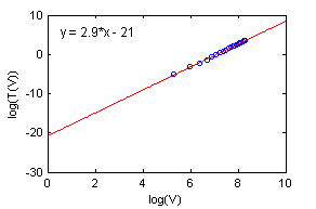
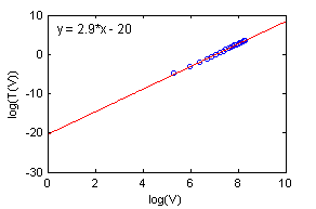
Figure 1. The time it takes to compute the spectrum of $\widetilde{L}$ as a function of the number of vertices, for two different connectivity densities: $\frac{r}{V}=0.5$ in the upper figure and $\frac{r}{V}=5$ in the lower figure.

Finally, we would like to show that the present method can be applied for counting nodal domains of functions defined on two dimensional grids and that its efficiency is comparable to that of the commonly used HK algorithm. Given a function f on a two dimensional domain, we have to compute its values on a rectangular grid with $\sqrt{V}\times\sqrt{V}$ points. The HK algorithm counts the nodal domains in $O(V)$ operations [30]. Using our method, we consider the rectangular grid as a graph with $V$ vertices. Assuming for simplicity periodic boundary conditions, the valency of all the vertices is 4. The corresponding $L$ matrix is a $V\times V$ matrix which is sparse (as long as $V\gg 4$), and due to the periodic boundary conditions it takes the explicit form:

(49) $$L_{i,j}=4\delta_{i,j}-\delta_{i,j-1}-\delta_{i,j+1}-\delta_{i-V,j}-\delta_{i+V,j}\ .$$

Thus, storing $L$ takes only $O(V)$ memory cells, and constructing $\widetilde{L}$ takes $O(V)$ operations. We mentioned above that for a general real symmetric matrix, the number of operations needed is $O(V^{\alpha})$, where $\alpha\simeq 2.3$ and at worst case $\alpha\simeq 3$. However, the sparse nature of $L$ significantly simplifies the problem. The most well-known eigenvalue method for sparse-real-symmetric matrices is the Lanczos method. In addition, in recent years, new efficient algorithms were discovered for the same problem. In [31], it is proven that finding the eigenvalues of a sparse symmetric matrix takes only $O(V)$ operations. Combining the costs, we find that it takes our algorithm $O(V)$ operations in order to compute the nodal domains count, and therefore it is comparable in efficiency to the HK algorithm.
As mentioned earlier, the labeling algorithms also display linear efficiency ([46],[47]). The labeling algorithms have the advantage that they are simpler in a sense, and that they are implemented quite easily as computer programs. In addition, the labeling algorithms maintain their linear efficiency even for graphs with dense Laplacians. It is worth mentioning, however, that our algorithm has the advantage that it provides an analytic expression of the nodal domains count (48).

4.4. Method IV. – A geometric point of view

The counting method proposed here uses a geometric point of view which starts by considering the $V$ dimensional Euclidean space, and dividing it into $2^{V}$ sectors using the following construction. Consider the $2^{V}$ vectors $\textbf{e}^{(\alpha)}=(e^{(\alpha)}_{1},e^{(\alpha)}_{2},\ldots,e^{(\alpha)}_{V})$ where $e^{(\alpha)}_{i}=\{1,-1\}$, $\alpha=1,2,\ldots,2^{V}$. A vector $\textbf{x}\in\mathbb{R}^{V}$ is in the sector $\alpha$ if $\textbf{x}\cdot\textbf{e}^{(\alpha)}=\sum_{i=1}^{V}{\mid x_{i}\mid}$. In two dimensions, the sectors are the standard quadrants. We shall refer to the vectors $\textbf{e}^{(\alpha)}$ as the indicators.

Given a graph $\mathcal{G}$ with $V$ vertices, we partition the $2^{V}$ indicators into disjoint sets: $\gamma_{n}=\{\textbf{e}^{(\alpha)}:\nu(\textbf{e}^{(\alpha)})=n\}$ where $\nu(\textbf{e}^{(\alpha)})$ denotes the nodal domains count of the indicator $\textbf{e}^{(\alpha)}$ with respect to $\mathcal{G}$. As shown before $\rm{max}\{n\,|\,\gamma_{n}\neq\emptyset\}\leq V-\chi+2$, where $\chi$ is the chromatic number of $\mathcal{G}$, and also some of the $\gamma_{i}^{{}^{\prime}}s$ might be empty.

Let f be a vector with non-zero entries defined on the vertex set of $\mathcal{G}$. Then, the main observation is that $\nu(\textbf{f})=n$ if and only if:

(50) $$\sum_{\textbf{e}^{\alpha}\in\gamma_{n}}\hat{\delta}\left(\left(\textbf{e}^{\alpha},\textbf{f}\right)-\sum_{i=1}^{V}\mid\textbf{f}_{i}\mid\right)\ =\ 1\ ,$$

where,

(51) $$\hat{\delta}(x)=\lim_{\epsilon\rightarrow 0}\frac{\epsilon}{x}\sin{\frac{x}{\epsilon}}=\left\{\begin{array}[]{ll}1,&\textrm{if $x=0$}\\ 0,&\textrm{if $x\neq 0$}\end{array}\right.\ .$$

and $\left(\textbf{e}^{\alpha},\textbf{f}\right)$ is the dot product of $\textbf{e}^{\alpha}$ and f. In other words, by finding the sector to which f belongs and knowing from a preliminary computation the number of nodal domains in each sector, one obtains the desired nodal count. Thus, the present method requires a preliminary computation in which the sectors are partitioned into equi-nodal sets $\gamma_{n}$. This should be carried out once for any graph. Therefore the method is useful when the nodal counts of many vectors is required. In several applications, one is given a vector field (of unit norm for simplicity) $\textbf{f}\in\mathbb{S}^{V-1}$ which is distributed on the $(V-1)$-sphere with a given probability distribution $p(\textbf{f})$, and one is asked to compute the distribution of nodal counts,

(52) $$P(n)=\int_{S^{V-1}}p(\textbf{f})\,\hat{\delta}\left(\nu(\textbf{f})-n\right)\,d^{V-1}\textbf{f}\ .$$

In such cases, the preliminary task of computing the equi-nodal pays off, and one obtains the following analytic expression for the distribution of the nodal counts.

(53) $$P(n)=\int_{S^{V-1}}p(\textbf{f})\,d^{V-1}\textbf{f}\sum_{\textbf{e}^{\alpha}\in\gamma_{n}}\hat{\delta}\left(\left(\textbf{e}^{\alpha},\textbf{f}\right)-\sum_{i=1}^{V}|\textbf{f}_{i}|\right)={}$$

$${}\int_{\mathbb{R}^{V}}\tilde{p}(\textbf{f})\,\delta\left(1-|\textbf{f}|^{2}\right)\,d^{V}\textbf{f}\sum_{\textbf{e}^{\alpha}\in\gamma_{n}}\hat{\delta}\left(\left(\textbf{e}^{\alpha},\textbf{f}\right)-\sum_{i=1}^{V}|\textbf{f}_{i}|\right)$$

where: $\tilde{p}(\textbf{f})=p(\frac{\textbf{f}}{|\textbf{f}|})\cdot 2|\textbf{f}|$.
(53) can also be formulated as:

(54) $$P(n)=\sum_{\beta=1}^{2^{V}}\int_{f_{i}\geq 0}\tilde{p}(\textbf{f}^{\beta})\,\delta(1-|\textbf{f}|^{2})\,d^{V}\textbf{f}\sum_{\textbf{e}^{\alpha}\in\gamma_{n}}\hat{\delta}\left(\left(\textbf{e}^{\alpha},\textbf{f}^{\beta}\right)-\sum_{i=1}^{V}f_{i}\right)={}$$

$${}\sum_{\textbf{e}^{\beta}\in\gamma_{n}}\int^{+}\tilde{p}(\textbf{f}^{\beta})\,\delta(1-|\textbf{f}|^{2})\,d^{V}\textbf{f}\sum_{\textbf{e}^{\alpha}\in\gamma_{n}}\hat{\delta}\left(\left(\textbf{e}^{\alpha},\textbf{f}^{\beta}\right)-\sum_{i=1}^{V}f_{i}\right)$$

Where $\int^{+}=\int_{f_{i}\geq 0}$ means integration on the first sector (the vectors with all entries positive) and $\textbf{f}^{\mu}=(f_{1}e_{1}^{\mu},f_{2}e_{2}^{\mu},\ldots,f_{V}e_{V}^{\mu})$.

Equations (53) and (54) are the general equations governing the nodal domains count distribution. In order to make further progress, we need to specify the distribution from which $\bf f$ is taken. This means that we need to specify $\tilde{p}(\textbf{f})$ in (53) for example. Let us discuss two examples:
A uniform distribution over the $V-1$ dimensional sphere: In this case, we can solve Equation (53) and get that $P(n)=\frac{|\gamma_{n}|}{2^{V}}$. Note that for a tree, we can solve this problem by other means. Using (20), we see that for a tree, the number of nodal domains is equal to the number of flips plus one. Since $\bf f$ is taken from the uniform distribution, then the probability of a flip is half. The number of flips in a vector $\bf f$ is thus a binomial variable: $\mathrm{F}(\textbf{f})\sim Binomial(N,p)$ with $N=V-1$ is the number of bonds, and $p=\frac{1}{2}$. For large enough $V$ this approaches the Gaussian distribution: $\mathrm{F}(\textbf{f})\sim Gaussian(\mu,\sigma^{2})$ with $\mu=\frac{V-1}{2}$ and $\sigma^{2}=\frac{V-1}{4}$. From this result we can infer that:

(55) $$P(n)\approx\frac{2}{\sqrt{2\pi(V-1)}}\exp{(\frac{-2(n-\frac{V+1}{2})^{2}}{V-1})}$$

(56) $$|\gamma_{n}|\approx\frac{2^{V+1}}{\sqrt{2\pi(V-1)}}\exp{(\frac{-2(n-\frac{V+1}{2})^{2}}{V-1})}$$

For the other extreme, the complete graph, $K_{V}$, the only possible nodal domains counts are one and two [28]. The vectors which yield a nodal domains count of one are vectors of constant sign. All other vectors yield a nodal domains count of two. Indeed, using (53) or (54) it is easy to be convinced that for the complete graph, $\gamma_{1}=2$ while $\gamma_{2}=2^{V}-2$. All other $\gamma_{n}$’s are empty.
Micro-canonical ensemble: In this case the vectors $\bf f$ are uniformly distributed on the energy shell, where we can also define a measurement tolerance factor, $\Delta$:

(57) $$p_{E}(\textbf{f})=\frac{\delta\left(E-|\left(\textbf{f},L\textbf{f}\right)-\Delta|\right)\,\delta\left(1-|\textbf{f}|^{2}\right)}{\int_{S^{V-1}}d^{V-1}\textbf{f}\,\,\delta\left(E-|\left(\textbf{f},L\textbf{f}\right)-\Delta|\right)}$$

In order to make use of this ensemble, further work must be done, for example, a natural way to order the functions of the ensemble.

5. The resolution of isospectrality

There are several known methods to construct isospectral yet different graphs. A review of this problem for discrete graphs can be found in [33]. The conditions under which the spectral inversion of quantum graphs is unique were studied previously. In [38, 39] it was shown that in general, the spectrum does not determine uniquely the length of the bonds and their connectivity. However, it was shown in [35] that quantum graphs whose bond lengths are rationally independent “can be heard” - that is - their spectra determine uniquely their connectivity matrices and their bond lengths. This fact follows from the existence of an exact trace formula for quantum graphs [40, 41]. Thus, isospectral pairs of non congruent graphs, must have rationally dependent bond lengths. An example of a pair of metrically distinct graphs which share the same spectrum was already discussed in [35].

The main method of construction of isospectral pairs is due to Sunada [34]. This method enabled the construction of the first pair of planar isospectral domains in $\mathbb{R}^{2}$ [36] which gave a negative answer to Kac’s original question: ‘Can one hear the shape of a drum?’ [37]. Later, it was shown that all the known isospectral domains in $\mathbb{R}^{2}$ [42, 43] which were also constructed using the Sunada method have corresponding isospectral pairs of quantum graphs [44]. An example of this correspondence is shown in figure 2.

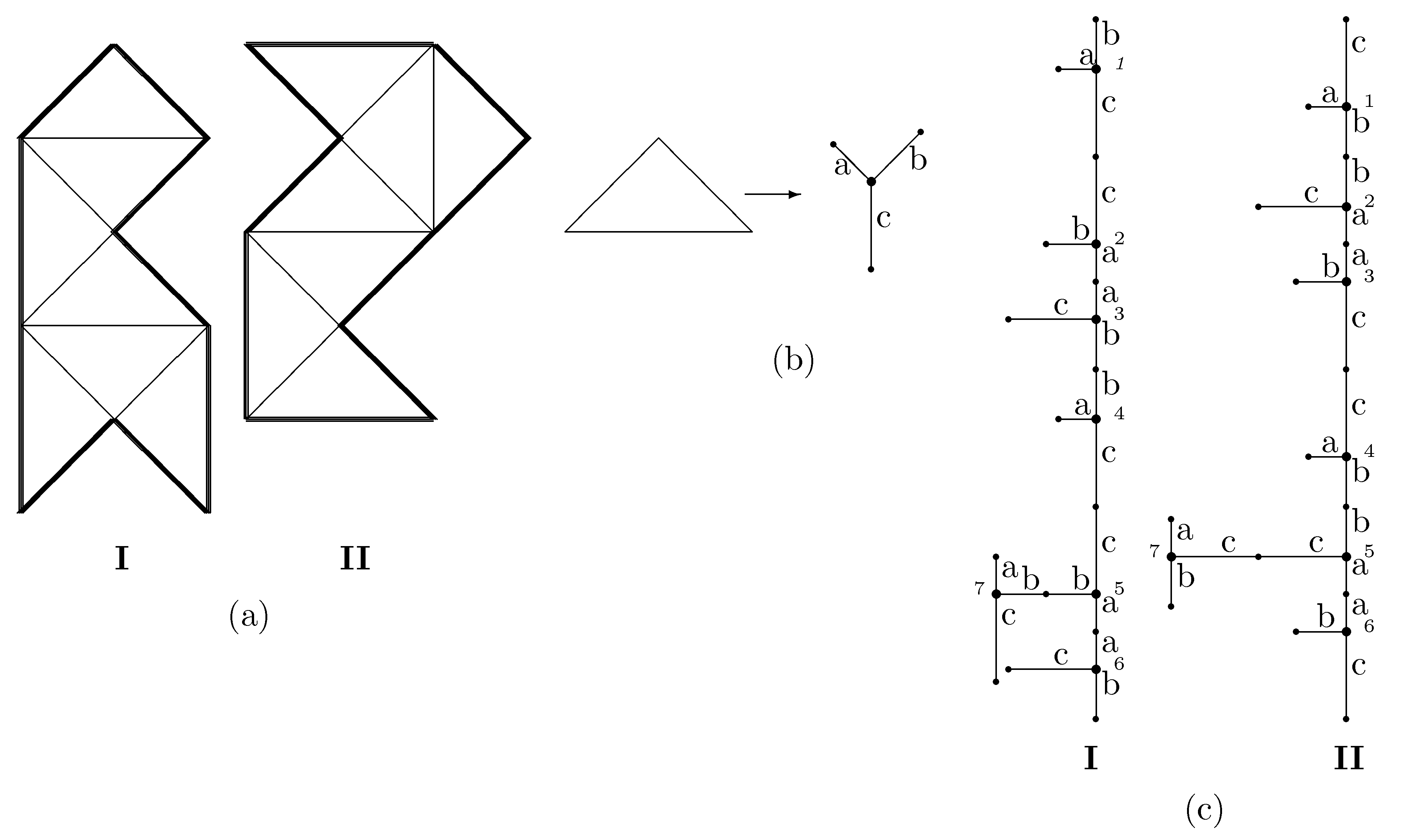
Figure 2. (a) Planar isospectral domains of the $7_{3}$ type. (b) Reducing the building block to a 3-star. (c) The resulting isospectral quantum graphs.

As mentioned in the introduction, it is conjectured [7, 19] that nodal domains sequences resolve between isospectral domains. For flat tori in 4-d, this was proven [8]. We present here three additional known results for the validity of the conjecture for graphs.

The first result is for the quantum graphs shown in figure 2(c). Both graphs of this isospectral pair are tree graphs and therefore have the same metric nodal count $\mu_{n}=n$ [15]. This demonstrates the need to use the discrete nodal count in order to resolve isospectrality in this case. Indeed numerical examination of this case shows that for the first 6600 eigenfunctions there is a different discrete nodal count for $\simeq$ 19 $\%$ of the eigenfunctions. Similar numerical results exist for two other pairs of isospectral graphs that are constructed from the isospectral domains in [42, 43]. The exact results are described in [19].

Another result is also in the field of quantum graphs [19]. The graphs in figure 3 are the simplest isospectral pair of quantum graphs known so far.

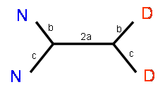
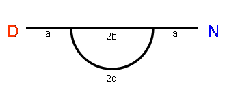
I                                                II

Figure 3. The isospectral pair with boundary conditions. D stands for Dirichlet and N for Neumann. The bonds’ lengths are determined by the parameters a,b,c

The simplicity of these graphs enables the comparison between the nodal counts of both graphs. It was proved that the nodal count is different between these graphs for half of the spectrum. This result was proved separately for the discrete count and for the metric count. The proof does not contain an explicit formula for the nodal count but rather deals with the difference of the nodal count between the graphs averaged over the whole spectrum.

Examining the nodal sequences for the graph $II$ for various values of the length parameters $a,b,c$, we observed that the formula

(58) $$\mu^{II}_{n}=n-\frac{1}{2}-\frac{1}{2}(-1)^{\lfloor\frac{b+c}{a+b+c}n\rfloor}$$

reproduces the entire data set without any flaw . Assuming it is correct (which is not yet proved rigorously) we first see that it provides an easy explanation for the previously discussed result regarding the resolution of isospectrality for this pair. For rationally independent values for the parameters a,b,c one gets that $\mu^{II}_{n}\neq n$ for half of the spectrum. Combining this with $\mu^{I}_{n}=n$ (since graph $I$ is a tree) we see again that for half of the spectrum the nodal domain sequences are different. Expression (58) is a periodic function of $n$ with period proportional to the length of the only loop orbit on the graph (the length is measured in units of the graph’s total length). It can be expanded and brought to a form which is similar in structure to a trace formula where the length of this orbit and its repetitions are the oscillation frequencies. A similar trace formula for the nodal counts of the Laplacian eigenfunctions on surfaces of revolution was recently derived [6].

Finally, we direct our attention to discrete Laplacians. It was recently shown [28] that if $\mathcal{G}$ and $\mathcal{H}$ are two isospectral graphs where one of them is bipartite and the other one is not, then their nodal domains count will differ. Without loss of generality, let $\mathcal{G}$ be a bipartite graph and $\mathcal{H}$ a non-bipartite one, then for the eigenvector of the largest eigenvalue, the nodal domains count are different: for $\mathcal{G}$, $\nu_{{}_{V}}=V$, while for $\mathcal{H}$, $\nu_{{}_{V}}<V$. The proof of this theorem is based on another interesting result derived in [28]: Denote by $\mathrm{\bf{f}}_{V}$ the eigenvector corresponding to the largest eigenvalue of the Laplacian of a connected graph $\mathcal{G}$. Then $\nu(\mathrm{\bf{f}}_{V})=\nu_{\mathcal{G}}=V$, if and only if $\mathcal{G}$ is bipartite. Figure 4. illustrates this result.

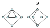
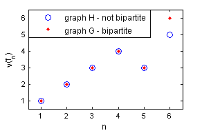
Figure 4. The upper figure presents a pair of isospectral graphs taken from [26]. Graph $G$, on the right is bipartite, whereas graph $H$, on the left, is not. The lower figure presents the nodal domains count, $\nu(\textbf{f}_{n})$ vs. the index $n$.

6. Summary and open questions

In spite of the progress achieved recently in the study of nodal domains on graphs, there are several outstanding open problems which call for further study. We list here a few examples.

Of fundamental importance is to find out whether there exists a “trace formula” for the nodal count sequence of graphs, similar to the one derived in [6] for surfaces of revolution. The closest we reached this goal is for the graph $II$ in the previous section, where (58) could be expanded in a Fourier series. However (58) was deduced numerically but not proved. Once a nodal trace formula is available, it could be compared to the spectral trace formula [41] and might show the way to prove or negate the conjecture that counting nodal domains resolves isospectrality [7, 19].

The conjecture mentioned above can be addressed from a different angle. One may study the various systematic ways to construct isospectral pairs and investigate the relations between the construction method and the nodal count sequence of the resulting graphs. Such an approach worked successfully for the isospectral graphs presented in figure 3 [19].

Another open question which naturally arises in the present context: Can one find graphs whose Laplacians have different spectra but the nodal count sequences are the same? A positive answer is provided for tree graphs [15]. Are there other less trivial examples of “isonodal” yet not isospectral domains?

It follows from Berkolaiko’s theorem [27] that the number of nodal domains (both metric and discrete) of the $n^{th}$ eigenfunction is bounded in the interval $[n-r,n]$. We can thus investigate the probability to have a nodal count $\nu_{n}=n-\tilde{r}$ (for $0\leq\tilde{r}\leq r$). This probability, which is defined with respect to a given ensemble of graphs, is denoted by $P(\tilde{r})$. It is defined for discrete graph Laplacians as:

(59) $$P(\tilde{r})\equiv\frac{1}{V}\langle\#\left\{\ 1\leq n\leq V:\ \nu_{n}=n-\tilde{r}\right\}\rangle\ .$$

The corresponding quantity for metric Laplacians is:

$$N(K) \equiv \langle\#\left\{n:k_{n}\leq K\right\}\rangle$$

$$P(\tilde{r};K) \equiv \frac{1}{N(K)}\ \langle\#\left\{\ n\leq N(K)\ :\ \mu_{n}=n-\tilde{r}\right\}\rangle$$

(60) $$P(\tilde{r}) \equiv \lim_{K\rightarrow\infty}P(\tilde{r};K)$$

Here, $\langle\ \ \ \rangle$ stands for the expectation with respect to the ensemble. New questions arise from the investigation of the relation between the connectivity of the graph and the nodal distribution $P(\tilde{r})$. Can one use the information stored in $P(\tilde{r})$ to gain information on the graphs e.g., the mean and the variance of the valency (degree) distribution of the vertices in the graphs?

Many of the results we have presented, have analogues in Riemannian manifolds (which in most cases, were discovered earlier) - for example, Courant’s theorem was originally formulated for manifolds. One can search for other analogues, and a good example is the Courant-Herrmann Conjecture (CHC). For manifolds the CHC states that any linear combination of the first $n$ eigenfunctions divide the domain, by means of its nodes, into no more than $n$ nodal domains. Gladwell and Zhu [45] have shown that in general there is no discrete counterpart to the CHC. However, we can still ask for which classes of graphs does the CHC hold?

7. Acknowledgments

The authors would like to thank L. Friedlander for stimulating discussions and suggestions of interesting open problems. It is a pleasure to acknowledge A. Aronovitch and Y. Elon for their helpful comments and well thought of critical remarks. We would like to thank the organizers of the AGA program of the I. Newton Institute, and in particular P. Kuchment for his support and encouragement. The work was supported by the Minerva Center for non-linear Physics and the Einstein (Minerva) Center at the Weizmann Institute, and by grants from the EPSRC (grant 531174), GIF (grant I-808-228.14/2003), and BSF (grant 2006065).

References

- [1] R. Courant and D. Hilbert, Methods of Mathematical Physics, Vol. 1, Interscience, New York, 1952.
- [2] A. Pleijel, Comm. Pure and Applied Math. 9,543(1956).
- [3] G. Blum, S. Gnutzman and U. Smilansky, Nodal Domains Statistics - A Criterion for Quantum Chaos, Physical Review Letters, Vol. 88, No. 11 March (2002).
- [4] E. Bogomolny and C. Schmit. Percolation Model for Nodal Domains of Chaotic Wave Functions. Phys. Rev. Lett. 88, 114102, 2002.
- [5] F. Nazarov, M. Sodin On the Number of Nodal Domains of Random Spherical Harmonics, arXiv:0706.2409v1.
- [6] S. Gnutzmann, Panos D. Karageorge and U. Smilansky, Can One Count the Shape of a Drum?, Physical Review Letters, Vol. 97, No. 9 August (2006)
- [7] S. Gnutzmann, U. Smilansky and N. Sondergaard, Resolving isospectral ‘drums’ by counting nodal domains, J. Phys. A.: Math. Gen. 38 (2005) 8921-8933.
- [8] J. Brüning, D. Klawonn and C. Puhle, Comment on “Resolving isospectral ‘drums’ by counting nodal domains”, J. Phys. A: Math. Theor. 40 (2007) 15143-15147.
- [9] T. Bykoglu, A discrete nodal domain theorem for trees, Linear Algebra and its Application 360 (2003) pp. 197-205
- [10] O. Al-Obeid, On the number of the constant sign zones of the eigenfunctions of a dirichlet problem on a network (graph), Tech. report, Voronezh: Voronezh State University, 1992, in Russian, deposited in VINITI 13.04.93, N 938 – B 93. – 8 p.
- [11] Y.V. Pokornyi, V.L. Pryadiev, and A. Al-Obeid, On the oscillation of the spectrum of a boundary value problem on a graph, Mat. Zametki 60 (1996), no. 3, 468–470, Translated in Math. Notes 60 (1996), 351–353.
- [12] Y.V. Pokornyi and V.L. Pryadiev, Some problems in the qualitative Sturm-Liouville theory on a spatial network, Uspekhi Mat. Nauk 59 (2004), no. 3(357), 115–150, Translated in Russian Math. Surveys 59 (2004), 515–552.
- [13] S. Gnutzmann and U, Smilansky, Quantum Graphs: Applications to Quantum Chaos and Universal Spectral Statistics. Advances in Physics 55 (2006) 527-625.
- [14] P. Kuchment, Quantum graphs: I. Some basic structures, Waves in Random Media 14, S107 (2004).
- [15] P. Schapotschnikow, Eigenvalue and nodal properties on quantum graph trees, Waves in Random and Complex Media, Vol. 16, No. 3, August (2006), pp. 167-178.
- [16] E. Brian Davies, Graham M.L. Gladwell, Josef Leydold and Peter F. Stadler, Discrete Nodal Domain Theorems, Linear Algebra and its Applications Vol. 336, October (2001), pp. 51-60.
- [17] S. Gnutzmann, U. Smilansky and J. Weber, Nodal counting on quantum graphs, Waves in Random and Complex Media, Vol. 14, No. 1, January (2004), pp. S61 - S73.
- [18] B. D. McKay, The expected eigenvalue distribution of a random labelled regular graph, Linear Algebra and its Applications, 40 (1981) 203-216.
- [19] R. Band, T. Shapira and U. Smilansky, Nodal domains on isospectral quantum graphs: the resolution of isospectrality?, J. Phys. A.: Math. Gen. 39 (2006) 13999-14014.
- [20] Dragos M. Cvetkovic, Michael Doob and Horst Sachs, Spectra of Graphs Theory and Applications, Academic press, New York, 1979.
- [21] B. Mohar, The Laplacian spectrum of graphs, in “Graph Theory, Combinatorics, and Applications”, Vol. 2, Ed. Y. Alavi, G. Chartrand, O. R. Oellermann, A. J. Schwenk, Wiley, 1991, pp. 871-898.
- [22] Fan R. K. Chung, Spectral Graph Theory, Regional Conference Series in Mathematics 92, American mathematical Society(1997).
- [23] T. Bykoglu, J. Leydold, and P.F. Stadler, Laplacian Eigenvectors of Graphs: Perron-Frobenius and Faber-Krahn Type Theorems, Series: Lecture Notes in Mathematics , Vol. 1915, (2007)
- [24] R. Roth, On the eigenvectors belonging to the minimum eigenvalue of an essentially nonnegative symmetric matrix with bipartite graph, Linear algebra Appl. 118:1-10, (1989)
- [25] T. Bykoglu, J. Leydold, and P.F. Stadler, Nodal Domain Theorems and Bipartite Subgraphs, Electronic Journal of Linear Algebra 13 (2005) pp. 344-351.
- [26] Willem H. Haemers, Edward Spence, Enumeration of cospectral graphs, European Journal of Combinatorics 25 (2004) 199-211
- [27] G. Berkolaiko, A lower bound for nodal count on discrete and metric graphs, math-ph/0611026 (2006).
- [28] I. Oren, Nodal domain counts and the chromatic number of graphs, J. Phys. A: Math. Theor. 40 (2007) 9825-9832.
- [29] J. Dongarra, F. Tisseur, Parallelizing the Divide and Conquer Algorithm for the Symmetric Tridiagonal Eigenvalue Problem on Distributed Memory Architectures, SIAM J.Sci. Comput. Vol. 20, No. 6, (1999) pp 2223-2236.
- [30] J. Hoshen, R. Kopleman, Phys. Rev. B 14 (1976) 3438.
- [31] Shing-Tung Yau and Ya Yan LU, A New Approach to Sparse Matrix Eigenvalues, Aerospace Control Systems, 1993. Proceedings. The First IEEE Regional Conference on May 25-27, 1993 pp 132 - 137.
- [32] G. Foltin, Counting nodal domains, nlin/0302049 (2003).
- [33] R. Brooks, Ann. Inst. Fouriere 49 707-725,(1999).
- [34] T. Sunada, Ann. of math. 121 196-186,(1985).
- [35] B. Gutkin and U. Smilansky J. Phys A.31, 6061-6068 (2001).
- [36] C. Gordon, D. Webb and S . Wolpert, Bull. Am. Math. Soc. 27 134-138 (1992).
- [37] M. Kac, Amer. Math. Monthly, 73 (1966) 1-23.
- [38] J. von Below in ”Partial Differential Equations on Multistructeres” Lecture notes in pure and applied mathematics, 219, Marcel Dekker Inc. New York, (2000) 19-36.
- [39] R. Carlson, Trans. Amer. Math. Soc. 351 4069-4088 (1999).
- [40] Jean-Pierre Roth, in: Lectures Notes in Mathematics: Theorie du Potentiel, A. Dold and B. Eckmann, eds. (Springer–Verlag) 521-539.
- [41] T. Kottos and U. Smilansky, Annals of Physics 274 76 (1999).
- [42] P. Buser, J. Conway, P. Doyle and K.-D. Semmler, Int. Math. Res. Notices 9 (1994), 391-400.
- [43] Y. Okada and A. Shudo J. Phys. A: Math. Gen. 34 (2001) 5911-5922.
- [44] Talia Shapira and Uzy Smilansky, Proceedings of the NATO advanced research workshop, Tashkent, Uzbekistan, 2004.
- [45] Gladwell, G.M.L. and Zhu, H.M., The Courant-Herrmann Conjecture, ZAMM. Math. Mech., 83 (2003) 275-281.
- [46] M.B. Dillencourt, H. Samet and M. Tamminen, A general approach to connected-component labeling for arbitrary image representations, J. ACM 39 (1992) 253-280, Corr. pp. 985-986.
- [47] C. Fiorio and J. Gustedtb, Two linear time Union-Find strategies for image processing, Theoretical Computer Science, 154, 2, (1996), 165-181.