Uniform approximation for the overlap caustic of a quantum state with its translations

Abstract

The semiclassical Wigner function for a Bohr-quantized energy eigenstate is known to have a caustic along the corresponding classical closed phase space curve in the case of a single degree of freedom. Its Fourier transform, the semiclassical chord function, also has a caustic along the conjugate curve defined as the locus of diameters, i.e. the maximal chords of the original curve. If the latter is convex, so is its conjugate, resulting in a simple fold caustic. The uniform approximation through this caustic, that is here derived, describes the transition undergone by the overlap of the state with its translation, from an oscillatory regime for small chords, to evanescent overlaps, rising to a maximum near the caustic. The diameter-caustic for the Wigner function is also treated.

I Introduction

It is often assumed that the Wigner function Wigner , $W({\mathbf{x}})$ in the phase plane ${\mathbf{x}}=(p,q)$, for a semiclassical WKB state can be approximated by a Dirac $\delta$-function on the corresponding classical closed curve in phase space. This simplest approximation does, indeed, lead to reliable expectation values for smooth classical observables. Nonetheless, it is hopelessly inadequate for the description of delicate interference effects that are becoming ever more accessible to experiments related to quantum information, either in quantum optics, atom traps, or other quickly developing technologies. It is then necessary to resort to more refined semiclassical descriptions for the phase space representations of quantum states, such as Berry’s uniform approximation for the Wigner function Berry77 .

A typical interference experiment superposes two modified copies of the same initial state (see e.g. Leonhardt ). For instance, in quantum optics, it is easy to achieve the unitary transformation that corresponds to a uniform phase space translation (or displacement). This translated state can then interfere with the original state. In general, the unitary translation operator

$$\hat{T}_{\mbox{\boldmath$\xi$}}=\exp{\left[\frac{i}{\mbox{\amsb\char 125\relax}}(\mbox{\boldmath$\xi$}\wedge\hat{{\mathbf{x}}})\right]}=\exp{\left[\frac{i}{\mbox{\amsb\char 125\relax}}(\mbox{\boldmath$\xi$}_{p}\cdot\hat{q}-\mbox{\boldmath$\xi$}_{q}\cdot\hat{p})\right]}\ ,$$ (1)

acts on the state $|\psi\rangle$ to produce the new state $|\psi_{\mbox{\boldmath$\xi$}}\rangle=\hat{T}_{\mbox{\boldmath$\xi$}}|\psi\rangle$ in strict correspondence to the classical translation: ${\mathbf{x}}\mapsto{\mathbf{x}}+\mbox{\boldmath$\xi$}$. Thus, given an arbitrary superposition of a state and its translation, $a|\psi\rangle+b|\psi_{\mbox{\boldmath$\xi$}}\rangle$, with $|a|^{2}+|b|^{2}=1$, the probability that this is measured to be in the untranslated state is $|a+b\langle\psi|\psi_{\mbox{\boldmath$\xi$}}\rangle|^{2}$.

Evidently, measurements of such probabilities (through repeated preparation) supply detailed quantum information concerning these initial states. It so happens that the full set of possible overlaps defines the complete phase space representation,

$$\chi(\mbox{\boldmath$\xi$})=\frac{1}{(2\pi\mbox{\amsb\char 125\relax})}\langle\psi|\hat{T}_{-\mbox{\boldmath$\xi$}}|\psi\rangle.$$ (2)

This is known as the chord function OzorioRep , the quantum characteristic function (or the Weyl function as in Choun ), which is the Fourier transform of the Wigner function:

$$\chi(\mbox{\boldmath$\xi$})=\frac{1}{(2\pi\mbox{\amsb\char 125\relax})}\int d{\mathbf{x}}\;W({\mathbf{x}})\exp{\left\{\frac{i}{\mbox{\amsb\char 125\relax}}(\mbox{\boldmath$\xi$}\wedge{\mathbf{x}})\right\}}\ .$$ (3)

The latter can be redefined, following Royer OzorioRep ; Royer , as

$$W({\mathbf{x}})=\frac{1}{(\pi\mbox{\amsb\char 125\relax})}\langle\psi|\hat{R}_{{\mathbf{x}}}|\psi\rangle,$$ (4)

where $\hat{R}_{{\mathbf{x}}}$, the Fourier transform of the translation operators, corresponds classically to the phase space reflection through the point ${\mathbf{x}}$, i. e. ${\mathbf{x}}_{0}\mapsto 2{\mathbf{x}}-{\mathbf{x}}_{0}$. An important consequence is that the phase space correlations Choun ; OzVaSa , for translational interference,

$$C({\mathbf{\xi}})=|\langle\psi|\psi_{\mbox{\boldmath$\xi$}}\rangle|^{2}=(2\pi\mbox{\amsb\char 125\relax})^{2}\int\rm d\mbox{\boldmath$\eta$}\;e^{i\mbox{\boldmath$\eta$}\wedge\mbox{\boldmath$\xi$}/\mbox{\amsb\char 125\relax}}\left|\chi(\mbox{\boldmath$\eta$})\right|^{2}=(2\pi\mbox{\amsb\char 125\relax})^{2}\int\rm d{\mathbf{x}}\>W({\mathbf{x}})\>W({\mathbf{x}}-\mbox{\boldmath$\xi$})\;,$$ (5)

coincide with the autocorrelation of the Wigner function itself. A study of interference phenomena using the quantum phase space formalism, besides some properties of phase space distributions can be found in Choun .

In the limit of small displacements, $\mbox{\boldmath$\xi$}\rightarrow 0$, the correlations attain their maximal value, $C(0)=1$. Increased translations reduce them to an oscillatory regime. We shall have be concerned with the correlation of states, whose chord function can be semiclassically approximated by OzVaSa ; Oz-enta

$$\chi(\mbox{\boldmath$\xi$})=\sum_{j}\;\alpha_{j}(\mbox{\boldmath$\xi$})\;e^{i{\sigma}_{j}(\mbox{\boldmath$\xi$})/\mbox{\amsb\char 125\relax}}=\sum_{j}\;\chi_{j}(\mbox{\boldmath$\xi$})\ ,$$ (6)

where the amplitudes and phases are determined by a classical curve, as will be described in the next section. This is similar to the simplest semiclassical approximation for the Wigner function Berry77

$$W({\mathbf{x}})=\sum_{j}\;a_{j}({\mathbf{x}})\;e^{iA_{j}({\mathbf{x}})/\mbox{\amsb\char 125\relax}}=\sum_{j}\;W_{j}({\mathbf{x}})\ .$$ (7)

Furthermore, the Fourier relation between this pair of representations is reflected in the reciprocal relation, which specifies the centres

$${\mathbf{x}}_{j}(\mbox{\boldmath$\xi$})={\mathbf{J}}\frac{\partial\sigma_{j}}{\partial\mbox{\boldmath$\xi$}}\ ,$$ (8)

for the realizations of the vector $\xi$ as a chord of the classical curve, whereas

$$\mbox{\boldmath$\xi$}_{j}({\mathbf{x}})=-{\mathbf{J}}\frac{\partial S_{j}}{\partial{\mathbf{x}}}\ .$$ (9)

determines the chords that have a given centre. Here,

$${\mathbf{J}}=\left(\begin{array}[]{cc}0&-1\\ 1&0\end{array}\right)\;$$ (10)

is the standard symplectic matrix. Typically for an energy eigenstate, the classical curve is a level curve for the corresponding classical Hamiltonian, related by Bohr-Sommerfeld VanVleck ; Maslov ; OzorioHam ; Gutzwiller quantization. In this way (6) and (7) are alternative phase space representation of WKB wave functions.

For large enough displacements, such that the classical translation of the curve does not intersect the original curve, the phase space correlations are negligible. The transition between this and the previous oscillatory regime takes place along a caustic where the chord function attains locally maximal amplitudes and the simple semiclassical approximation (6) breaks down. The main purpose of this paper is to establish the correct description of this transition from the oscillatory regime to the region of negligible overlap through a uniform approximation. It is interesting that the caustic region for increased quantum correlations is entirely determined by the geometry of the classical curve supporting the quantum state. It will here be assumed that this curve is convex, so that the locus of its diameters, i.e. its maximal chords, also defines a closed convex curve.

The present approximation has some resemblance to the uniform approximation obtained by Berry Berry77 for the Wigner function close to the classical curve. However, the latter is simplified by symmetry constraints that do not hold here. Indeed, the present treatment is even closer to the uniform approximation along the caustic of the Wigner function far from the curve, which will also be treated. For a start, section 2 reviews the geometrical construction of the Wigner function and the chord function for a state that corresponds to a closed quantized curve. In contrast to the treatment in Berry77 , the construction of the present uniform approximations cannot be limited to a single WKB branch.

Having defined geometrically the stationary phases for the Wigner function and the chord function, the method of Chester, Friedman and Ursell Chester then supplies uniform approximations for the chord function in terms of the Airy function and its derivative in section 3 and for the Wigner function in section 4. In both cases, the asymptotic form of these functions for large argument are then connected to the simpler semiclassical forms (6) and (7). The analysis of these uniform approximations close to the caustic furnishes simpler transitional approximations in section 5.

None of these expressions extends right down to the limit of small chords, because this is another caustic for both the Wigner function and the chord function. However, for the eigenstates of the harmonic oscillator (Fock states), the approximations for large chords can be compared to a small chord formula specified by a Bessel functionOzVaSa . This leads to a discussion in section 6 of the normalization of all these phase space approximations, deriving from the limit $C(0)=1$.

II Construction of the semiclassical Wigner and chord functions

Before embarking on uniform approximations for the Wigner and chord functions, it is worthwhile to review the derivation of the simpler semiclassical formulae presented in the introduction. Thus we also specify explicitly the amplitudes and phases and their geometric interpretation, which are essential ingredients of the uniform approximations.

The starting point is the generalized WKB expression for the wave function VanVleck ; Maslov ; OzorioHam ; Gutzwiller ,

$$\left\langle q\big{|}\psi_{I}\right\rangle=N\sum_{j}\left|\frac{\partial^{2}S_{j}(q,I)}{\partial q\partial I}\right|^{\frac{1}{2}}\exp\left[\frac{i}{\mbox{\amsb\char 125\relax}}S_{j}(q,I)+i\beta_{j}\right].$$ (11)

Here we assume that the classical curve is defined as a level curve of the action variable $I({\mathbf{x}})$, such that $S_{j}(q,I)$ corresponds to the $j$’th branch of the generating function for the canonical transformation $(p,q)\mapsto(I,\theta)$, $\beta_{j}$ is the Maslov correction and $N$ is the overall normalization constant. Choosing the arbitrary initial point, $q_{0}$, the action branches are defined as

$$S_{j}(q,I)=\int_{q_{0}}^{q}p_{j}(Q,I)\;dQ,\quad\quad\frac{\partial S_{j}}{\partial I}=\theta_{j},\quad\quad\frac{\partial S_{j}}{\partial q}=p_{j},$$ (12)

so that the amplitude can be rewritten in terms of

$$\frac{\partial^{2}S_{j}(q,I)}{\partial q\partial I}=\frac{\partial p_{j}}{\partial I}(q)=\left[\frac{\partial I}{\partial p}(p_{j}(q),q)\right]^{-1}.$$ (13)

It will be assumed that the state corresponds classically to a convex closed curve, so that there will always be a single pair of branches for the action function. This will hold irrespective of any linear canonical transformation, which it may be convenient to make, given that both the chord function and the Wigner functions are covariant with respect to such changes of phase space coordinates. It will also be important to recall that the closed curve must satisfy the Bohr-Sommerfeld quantization condition:

$$\oint p\,dq=2\pi\mbox{\amsb\char 125\relax}\left(n+\frac{1}{2}\right),\quad\quad\quad n\in\mathbb{Z}.$$ (14)

Expressing the translation and reflection operators within the position representation (see e.g. OzorioRep ), the chord function (2) becomes

$$\chi(\xi)=\frac{1}{(2\pi\mbox{\amsb\char 125\relax})}\int dq\left\langle q^{+}\big{|}\psi_{I}\right\rangle\left\langle\psi_{I}\big{|}q^{-}\right\rangle e^{-i\bm{\xi}_{p}\cdot q/\mbox{\amsb\char 125\relax}}$$ (15)

while the Wigner (4) is given by

$$W({\mathbf{x}})=\frac{1}{(\pi\mbox{\amsb\char 125\relax})}\int d\bm{\xi}_{q}\left\langle q^{+}\big{|}\psi_{I}\right\rangle\left\langle\psi_{I}\big{|}q^{-}\right\rangle e^{-ip\cdot\bm{\xi}_{q}/\mbox{\amsb\char 125\relax}}$$ (16)

where, in both equations $q^{\pm}=q\pm\bm{\xi}_{q}/2$.

In the semiclassical limit, the WKB expression can be inserted, so that we obtain in each case a sum of integrals that are dominated by their points of stationary phase. Irrespective of whether these points are sufficiently isolated so as to allow for immediate evaluation by the stationary phase method, we need to understand the geometric construction that defines them. In both cases, each stationary point defines values of $q^{\pm}$ pairs, which are $q$-coordinates of a pair of points, ${\mathbf{x}}^{\pm}$, lying on the classical closed curve. In the case of the chord function, each ${\mathbf{x}}^{-}$ is the intersection of the classical curve with its uniform translation by the vector $-\mbox{\boldmath$\xi$}$, whereas ${\mathbf{x}}^{+}={{\mathbf{x}}^{-}}+\mbox{\boldmath$\xi$}$. This geometry is exhibited in Fig. 1, which shows that each chord has two realizations in a convex closed curve. Thus, this construction on a given convex curve always specifies a pair of centres ${\mathbf{x}}_{1}(\mbox{\boldmath$\xi$})$ and ${\mathbf{x}}_{2}(\mbox{\boldmath$\xi$})$ for each chord $\xi$ that can be fitted in the curve.

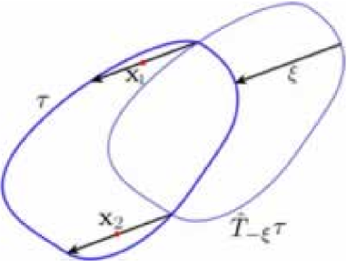
Figure 1: Geometrical construction for the stationary points of the chord function. The intersections at ${{\mathbf{x}}_{1}}^{-}$ and ${{\mathbf{x}}_{2}}^{-}$, of the closed curve with its translation by $-\mbox{\boldmath$\xi$}$, define the pair of realizations of this chord. The $q$-coordinate of the centres, ${{\mathbf{x}}_{1}}$ and ${\mathbf{x}}_{2}$ of these realizations defines the stationary points.

In the case of the Wigner function, instead of a translation, the classical curve is reflected through the reflection centre, ${\mathbf{x}}$. This results in a pair of intersections, ${\mathbf{x}}^{+}$ and ${\mathbf{x}}^{-}$, such that ${\mathbf{x}}$ is the centre for the pair of chords $\mbox{\boldmath$\xi$}=\pm({\mathbf{x}}^{+}-{\mathbf{x}}^{-})$. The stationary points are then the $q$-coordinates for this pair of chords. This geometry is shown in Fig. 2. Therefore, there will be at least one pair of chords $\pm\mbox{\boldmath$\xi$}({\mathbf{x}})$, for each reflection centre in the curve.

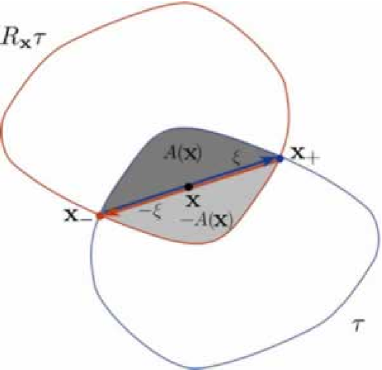
Figure 2: Geometrical construction for the stationary points of the Wigner function. The intersections of the closed curve with its reflection through ${\mathbf{x}}$ defines pair of chords centred on ${\mathbf{x}}$. The $q$-coordinate of these chords defines the stationary points. The area $A({\mathbf{x}})$ determines the phase of the Wigner function.

The stationary phase evaluation of each integral for the Wigner function,

$$W_{ij}({\mathbf{x}})=\frac{N^{2}}{2\pi\mbox{\amsb\char 125\relax}}\int d\bm{\xi}_{q}\left|\frac{\partial I}{\partial p}(p_{i}(q^{+}),q^{+})\frac{\partial I}{\partial p}(p_{j}(q^{-}),q^{-})\right|^{\frac{1}{2}}\exp\left[\frac{i}{\mbox{\amsb\char 125\relax}}\left[S_{i}(q^{+},I)-S_{j}(q^{-},I)-p\cdot\bm{\xi}_{q}+\beta_{i}-\beta_{j}\right]\right],$$ (17)

can usually be obtained from a single branch of the action function for the closed curve, that is, $i=j$. The stationary phase is half of the area between the curve and its reflection, or the “chord area” as shown in Fig. 2, except for a Maslov correction. The only difference between both phases, corresponding to $\pm\mbox{\boldmath$\xi$}({\mathbf{x}})$, is the sign, so that the semiclassical approximation is real Berry77 .

In the case of the chord function, each stationary phase is given by the construction in Fig. 3.

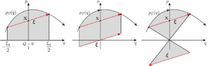
Figure 3: Several geometrical interpretations for the phase for the semiclassical chord function in the simpler approximation for a WKB function, considering one branch. The stationary phase itself is determined by the shaded area in the three casesOzVaSa .

Unlike the Wigner function, this depends explicitly on a change of phase space origin, ${\mathbf{x}}\mapsto{\mathbf{x}}+\mbox{\boldmath$\xi$}^{\prime}$, according to the exact formula OzVaSa ,

$$\chi_{\mbox{\boldmath$\mbox{\boldmath$\xi$}$}^{\prime}}(\mbox{\boldmath$\xi$})=e^{\frac{i}{\mbox{\amsb\char 125\relax}}\mbox{\boldmath$\mbox{\boldmath$\xi$}$}^{\prime}\wedge\mbox{\boldmath$\xi$}}\;\chi(\mbox{\boldmath$\xi$}),$$ (18)

but it is also covariant with respect to homogeneous linear canonical transformations.

The amplitudes in the above semiclassical approximations are best expressed in terms of the canonical action variable, $I({\mathbf{x}})$, that defines the closed curve and is conjugate to the angle variable $\theta({\mathbf{x}})$ along the curve. If we now define the transported action variable,

$$I^{\pm}=I({\mathbf{x}}\pm\mbox{\boldmath$\xi$}/2),$$ (19)

then, generally, the Poisson bracket for this pair of functions,

$$\{I^{+},I^{-}\}=\frac{\partial I^{+}}{\partial{\mathbf{x}}}\wedge\frac{\partial I_{-}}{\partial{\mathbf{x}}}\neq 0,$$ (20)

and it is found that these amplitudes in (6) and (7) are

$$a({\mathbf{x}})=|\{I^{+},I^{-}\}|^{-\frac{1}{2}}=\alpha(\mbox{\boldmath$\xi$}).$$ (21)

The difference between considering the amplitude as a function on ${\mathbf{x}}$ or $\xi$ depends on which variable is fixed in (21). This only changes the sign of the Poisson bracket. Here, the equality of coefficients for both representations holds for the chord and its centre, between a specific pair of points $({\mathbf{x}}^{-},{\mathbf{x}}^{+})$ on the closed curve.

A neat interpretation for these amplitudes follows from the identification of the action variable $I({\mathbf{x}})$ with a classical Hamiltonian. Then the closed curve becomes a closed trajectory, tangent to the phase space velocity vector, $\dot{{\mathbf{x}}}$, and

$$\{I^{-},I^{+}\}=\dot{\mathbf{x}}^{-}\wedge\dot{\mathbf{x}}^{+},$$ (22)

as shown in Fig. 4.

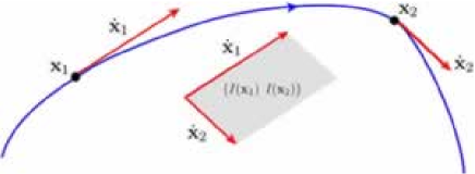
Figure 4: Geometrical interpretation for the semiclassical amplitudes of both the Wigner function and the chord function.

It follows that the amplitudes $\alpha_{j}(\mbox{\boldmath$\xi$})$ (or $a_{j}({\mathbf{x}})$), depend on the degree of transversality of the intersection between the curve and its translation, or its reflection Berry77 ; OzVaSa and so they diverge at caustics, where $\dot{\mathbf{x}}^{+}$ and $\dot{\mathbf{x}}^{-}$ are parallel.

So far, we have presumed that the contribution of each stationary phase point to the integrals for either the Wigner function or the chord function, can be obtained by considering a single branch of the WKB wave function. Thus, $i=j$ in (17) and this single branch can always be accessed through a canonical phase space rotation in the simple semiclassical approximations above and even for Berry’s uniform theory for the caustic that arises in the limit of small chords Berry77 . However, this is not possible in the present treatment of the caustic at maximal chords, where (21) also diverges for both representations, because the tips of the stationary chord become turning points for the WKB function in this limit. It is thus necessary to study this limit with the aid of phase space coordinates, such that it is the cross term between the pair of different branches, of the action function, which have stationary phases in (17). For this reason it will be important to take care of the phase relation between the branches across a turning point:

$$\left\langle q\big{|}\psi_{I}\right\rangle=N\left[\left|\frac{\partial^{2}S_{+}(q,I)}{\partial q\partial I}\right|^{\frac{1}{2}}\exp\left[\frac{i}{\mbox{\amsb\char 125\relax}}S_{+}(q,I)\right]+{\rm e}^{i\pi/2}\;\left|\frac{\partial^{2}S_{-}(q,I)}{\partial q\partial I}\right|^{\frac{1}{2}}\exp\left[\frac{i}{\mbox{\amsb\char 125\relax}}S_{-}(q,I)\right]\right],$$ (23)

where $\pi/2$ is the Maslov phase and $N$ is the normalization constant. Inserting the above wave function in (15), we obtain four integrals to evaluate. An appropiate choice of the coordinate axes orientation, in which the both of chord realizations are crossed, reduces the chord function for (23) to the single integral

$$\chi(\mbox{\boldmath$\xi$}) = \frac{N^{2}}{2\pi\mbox{\amsb\char 125\relax}}\int dq\left|\frac{\partial I}{\partial p}(p_{+}(q^{+}),q^{+})\frac{\partial I}{\partial p}(p_{-}(q^{-}),q^{-})\right|^{\frac{1}{2}}$$ (24)

$$\hskip 28.45274pt\times\exp\left(\frac{i}{\mbox{\amsb\char 125\relax}}\left[S_{+}(q^{+},I)-S_{-}(q^{-},I)-\bm{\xi}_{p}\cdot q\right]+i\frac{\pi}{2}\right).$$

Here $q^{\pm}=q\pm\mbox{\boldmath$\xi$}_{q}/2$. As stated previously, this geometry can be guaranteed by a phase space rotation. The evaluation of the chord areas in the Wigner function and the chord function for this geometry is discussed in Appendix A.

III Uniform approximation for the chord function

Let us allow the pair of these stationary points of (24) to coalesce for the chord $\mbox{\boldmath$\xi$}_{D}$, that corresponds to a diameter of the closed curve, i.e. a maximal chord, at which the semiclassical amplitude (21) diverges. In the present case of a convex curve, these diameters are the locus of a fold caustic with no higher singularity. This is simpler than the geometry for the corresponding caustic of the Wigner function, studied in the following section.

We also simplify the calculation by an appropriate choice of origin, in view of the simple translation property (18) of the chord function. This ideal origin lies midway between the centres for the pair of chord realizations, shown in Fig. 5.

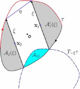
Figure 5: The difference in chord areas, $\mathcal{A}_{12}$, coincides with the area between the closed curve and its translation. This area shrinks to zero when $\xi$ becomes a diameter and its conjugate chord $\eta={\mathbf{x}}_{1}-{\mathbf{x}}_{2}\rightarrow 0$. The simplest choice of phase space origin is at midpoint between ${\mathbf{x}}_{1}$ and ${\mathbf{x}}_{2}$.

The pair of stationary points $q_{1}$ and $q_{2}$ of the integrand in (24) are solutions of the equation:

$$p_{+}(q+{\xi_{q}}/2)-p_{-}(q-{\xi_{q}}/2)=\xi_{p},$$ (25)

which are identified as the position coordinates of ${\mathbf{x}}_{1}$ and ${\mathbf{x}}_{2}$ in Fig. 5. According to Appendix A, the Bohr-Sommerfeld quantization rule (14) leads to the corresponding phases as

$$S_{+}(q_{1}+{\xi_{q}}/2)-S_{-}(q_{1}-{\xi_{q}}/2)-{\xi_{p}}q_{1}=\mathcal{A}_{1}(\xi)+{\mathbf{x}}_{1}\wedge\xi,$$ (26)

$$S_{+}(q_{2}+{\xi_{q}}/2)-S_{-}(q_{2}-{\xi_{q}}/2)-{\xi_{p}}q_{2}=\mathcal{A}_{2}(\xi)+{\mathbf{x}}_{2}\wedge\xi.$$ (27)

Instead of evaluating (24) by stationary phase, this integral is mapped onto the standard form for a fold diffraction catastrophe Berry76 :

$$\chi(\xi)=\frac{N^{2}}{2\pi i\mbox{\amsb\char 125\relax}}\exp\left(\frac{i\Sigma\mathcal{A}}{2\mbox{\amsb\char 125\relax}}\right)\int_{-\infty}^{\infty}du\;g(u;\xi)\;e^{i\left[\frac{u^{3}}{3}-\zeta\,u\right]},$$ (28)

where we have defined

$$\Sigma\mathcal{A}=\mathcal{A}_{1}+\mathcal{A}_{2},\quad\quad\frac{2}{3}\zeta(\mbox{\boldmath$\xi$})^{\frac{3}{2}}=\frac{\mathcal{A}_{12}}{2\mbox{\amsb\char 125\relax}}=\frac{\mathcal{A}_{1}-\mathcal{A}_{2}+\mbox{\boldmath$\eta$}\wedge\mbox{\boldmath$\xi$}}{2\mbox{\amsb\char 125\relax}}.$$ (29)

The action difference, $\mathcal{A}_{12}$, is the main ingredient in the present application of the method of uniform approximation Chester ; Berry76 . Its geometric definition is the area between the closed curve and its translation, as shown in Fig. 5. At the caustic, the chord $\mbox{\boldmath$\xi$}=\mbox{\boldmath$\xi$}_{D}$ is maximal and its conjugate chord OzVaSa : $\eta={\mathbf{x}}_{1}-{\mathbf{x}}_{2}\rightarrow 0$.

The above integral would define an Airy function abramowitz , Ai$(\zeta)$, if $g(u;\xi)=1$, but here the mapping between the variables $q\mapsto u$, respectively in (24) and (28), leads to

$$g(u;\xi)=\left|\frac{\partial I}{\partial p}(q(u)+{\xi_{q}}/2)\frac{\partial I}{\partial p}(q(u)-{\xi_{q}}/2)\right|^{-\frac{1}{2}}\frac{dq}{du}.$$ (30)

The approximation now consists in replacing this by a linear function which coincides with $g(u;\xi)$ at the stationary points, $\pm\zeta^{\frac{1}{2}}$ of (28). These map onto $q(\zeta^{\frac{1}{2}})={\mathbf{x}}_{1q}\equiv q_{1}$ and $q(-\zeta^{\frac{1}{2}})={\mathbf{x}}_{2q}\equiv q_{2}$. The Jacobian of the mapping $q\leftrightarrow u$ at the stationary points is specified by

$$\frac{dq}{du}(\zeta^{\frac{1}{2}}) = \left|\frac{2\mbox{\amsb\char 125\relax}\zeta^{\frac{1}{2}}}{\frac{\partial p}{\partial q}(q_{1}+{\xi_{q}}/2)-\frac{\partial p}{\partial q}(q_{1}-{\xi_{q}}/2)}\right|^{\frac{1}{2}},$$ (31)

$$\frac{dq}{du}(-\zeta^{\frac{1}{2}}) = \left|\frac{2\mbox{\amsb\char 125\relax}\zeta^{\frac{1}{2}}}{\frac{\partial p}{\partial q}(q_{2}+{\xi_{q}}/2)-\frac{\partial p}{\partial q}(q_{2}-{\xi_{q}}/2)}\right|^{\frac{1}{2}},$$ (32)

so that

$$g(\zeta^{\frac{1}{2}};\xi)=\left|\frac{2\mbox{\amsb\char 125\relax}\zeta^{\frac{1}{2}}}{\{I^{+}_{1},I^{-}_{1}\}}\right|^{\frac{1}{2}},\quad g(-\zeta^{\frac{1}{2}};\xi)=\left|\frac{2\mbox{\amsb\char 125\relax}\zeta^{\frac{1}{2}}}{\{I^{+}_{2},I^{-}_{2}\}}\right|^{\frac{1}{2}}.$$ (33)

Thus, recalling the definition of the transported action (19) for each chord realization, we now define

$$\Delta I^{12}\equiv\left|\{I_{1}^{+},I_{1}^{-}\}\right|^{-\frac{1}{2}}-\left|\{I_{2}^{+},I_{2}^{-}\}\right|^{-\frac{1}{2}}\quad\textrm{and }\quad\Sigma I^{12}\equiv\left|\{I_{1}^{+},I_{1}^{-}\}\right|^{-\frac{1}{2}}+\left|\{I_{2}^{+},I_{2}^{-}\}\right|^{-\frac{1}{2}},$$ (34)

so as to obtain

$$g(u;\xi) \simeq\sqrt{\frac{\mbox{\amsb\char 125\relax}}{2}}\left(\zeta^{\frac{1}{4}}\Sigma I^{12}+\frac{u}{\zeta^{\frac{1}{4}}}\Delta I^{12}\right),$$ (35)

as an approximation to (30), which is linear with respect to $u$ and has the correct values at the stationary points. Thus, the integral for the chord function becomes

$$\chi(\xi) = \frac{N^{2}}{ih}\frac{\sqrt{\mbox{\amsb\char 125\relax}}}{\sqrt{2}}\exp\left(i\frac{\Sigma\mathcal{A}}{2\mbox{\amsb\char 125\relax}}\right)\int_{-\infty}^{\infty}du\,\left(\zeta^{\frac{1}{4}}\Sigma I^{12}+\frac{u}{\zeta^{\frac{1}{4}}}\Delta I^{12}\right)\,e^{i\left[\frac{u^{3}}{3}-\zeta\,u\right]}$$ (36)

$$= \frac{N^{2}}{i}\frac{1}{\sqrt{2\mbox{\amsb\char 125\relax}}}\exp\left(i\frac{\Sigma\mathcal{A}}{2\mbox{\amsb\char 125\relax}}\right)\,\left(\zeta^{\frac{1}{4}}\Sigma I^{12}{\rm Ai}\left(-\zeta\right)-\frac{i}{\zeta^{\frac{1}{4}}}\Delta I^{12}{\rm Ai}^{\prime}\left(-\zeta\right),\right)$$

where ${\rm Ai}^{\prime}$ is the derivative of the Airy function. Finally, recalling the definition of the intermediate variable, $\zeta$, in terms of areas (29), we obtain the full unitary approximation for the chord function:

$$\chi(\mbox{\boldmath$\xi$})=N^{2}\exp\left(i\frac{\Sigma\mathcal{A}}{2\mbox{\amsb\char 125\relax}}\right)\,\left[\frac{\left[\frac{3}{4}\mathcal{A}_{12}\right]^{\frac{1}{6}}\Sigma I^{12}}{i\sqrt{2}\mbox{\amsb\char 125\relax}^{\frac{2}{3}}}{\rm Ai}\left(-\left[\frac{3\mathcal{A}_{12}}{4\mbox{\amsb\char 125\relax}}\right]^{\frac{2}{3}}\right)\right.-\left.\frac{\left[\frac{3}{4}\mathcal{A}_{12}\right]^{-\frac{1}{6}}\Delta I^{12}}{\sqrt{2}\mbox{\amsb\char 125\relax}^{\frac{1}{3}}}{\rm Ai}^{\prime}\left(-\left[\frac{3\mathcal{A}_{12}}{4\mbox{\amsb\char 125\relax}}\right]^{\frac{2}{3}}\right)\right].$$ (37)

The Airy function, ${\rm Ai}\left(-\zeta\right)$, oscillates with increasing amplitude as its argument increases and then decays exponentially for positive values of $-\zeta$. The maximum amplitude, just bellow the origin, indicates the singularity of the simple semiclassical amplitude at the caustic. In this region the second term depending on ${\rm Ai}^{\prime}\left(-\zeta\right)$ can be neglected, but it is necessary to obtain the correct limiting behaviour in the oscillatory region where the simple semiclassical description is valid. This term is a new feature in comparison with the uniform approximation for the Wigner function for small chords Berry77 , where it is absent because of the reflection symmetry. The other novel feature is the oscillatory phase proportional to $\Sigma\mathcal{A}$ along the caustic, which will be important to separate the contribution of each realization at the oscillatory regime. Indeed in the case when the chord areas are significantly greater than Planck’s constant, the functions in (37) can be replaced by the asymptotic forms for large negative values abramowitz ,

$${\rm Ai}(-x)\to\frac{1}{\sqrt{\pi}x^{\frac{1}{4}}}\cos\left(\frac{2}{3}x^{\frac{3}{2}}-\frac{\pi}{4}\right)\quad\textrm{and \;}\quad{\rm Ai}^{\prime}(-x)\to\frac{x^{\frac{1}{4}}}{\sqrt{\pi}}\sin\left(\frac{2}{3}x^{\frac{3}{2}}-\frac{\pi}{4}\right),$$ (38)

in order to obtain the correct form in the oscillatory regime as in (6):

$$\chi(\xi)\to\frac{N^{2}}{i\sqrt{2\pi\mbox{\amsb\char 125\relax}}}\left[\frac{\exp\left(i\left[\frac{\mathcal{A}_{1}}{\mbox{\amsb\char 125\relax}}-\frac{\pi}{4}\right]\right)}{|\{I^{+}_{1},I^{-}_{1}\}|^{\frac{1}{2}}}+\frac{\exp\left(i\left[\frac{\mathcal{A}_{2}}{\mbox{\amsb\char 125\relax}}+\frac{\pi}{4}\right]\right)}{|\{I^{+}_{2},I^{-}_{2}\}|^{\frac{1}{2}}}\right].$$ (39)

This result corresponds to the sum of contributions for each chord realization in the simpler stationary phase approximation of the semiclassical chord function in OzVaSa , where it was considered that each chord realization lies on a single of the WKB wave function.

IV Uniform approximation for the Wigner function

As the Wigner function is evaluated at a point ${\mathbf{x}}$ that lies further and further inside a convex closed classical curve, a caustic will be crossed. This is typically a cusped triangleBerry77 , in which there are three chords for each centre, as shown in Fig. 6. Generic paths to its interior enter the triangle through a fold caustic joining two cusps. Such a caustic point $\{{\mathbf{x}}_{i}\}$ is the centre of a diameter, as show in Fig. 6, as well being the centre of the other chord, which was followed in the continuous path through the caustic. An example of the full fringe pattern where the regions characterized by one or three chords are clearly discernible can be found in Oz-enta .

The uniform approximation to be derived here concerns the pair of chords, $\mbox{\boldmath$\xi$}_{1}$ and $\mbox{\boldmath$\xi$}_{2}$ in Fig. 7, that are born from the diameter at the caustic. Away from the cusps, the contribution of the separate chord, $\mbox{\boldmath$\xi$}_{3}$ in Fig. 7, can still be evaluated by stationary phase. This is just a simple semiclassical contribution,

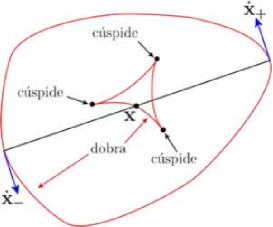
Figure 6: Wigner function catastrophes for a closed curve. The curve itself is a fold (short-chord catastrophe). Another singular curve lying in the interior is composed of folds and cusps (long-chord catastrophe). The catastrophe points correspond to centres of the diameters of the classical curve.

$$W_{3}({\mathbf{x}})=\frac{4N^{2}}{\sqrt{h}}\left|\{I({\mathbf{x}}+\mbox{\boldmath$\xi$}_{3}/2),I({\mathbf{x}}-\mbox{\boldmath$\xi$}_{3}/2)\}\right|^{-\frac{1}{2}}\cos\left(\frac{A_{3}}{\mbox{\amsb\char 125\relax}}-\frac{\pi}{4}\right),$$ (40)

which could be obtained from a single WKB branch, $i=j$ in (17). This could also be derived from a cross-branch $i\neq j$ (by rotating the phase space coordinates) from the same integral that furnishes the joint contribution of the pair of chords, $\mbox{\boldmath$\xi$}_{1}$ and $\mbox{\boldmath$\xi$}_{2}$, which coalesce at the diameter $\mbox{\boldmath$\xi$}_{D}$.

This crossed chord picture is essential for the uniform approximation. As in the theory for the chord function, we now map the integral in the region corresponding to the chords $\mbox{\boldmath$\xi$}_{1}$ and $\mbox{\boldmath$\xi$}_{2}$ onto the diffraction integral, as in (28).

$$W({\mathbf{x}})=2\Re\mathfrak{e}\frac{N^{2}}{i2\pi\mbox{\amsb\char 125\relax}}{\exp\left(i\frac{\Sigma A}{2\mbox{\amsb\char 125\relax}}\right)}\int_{-\infty}^{\infty}dz\,g(z;{\mathbf{x}})\,e^{i\left[\frac{z^{3}}{3}-\zeta z\right]}+W_{3}({\mathbf{x}}).$$ (41)

Here the parameters of the transformation are given by

$$\Sigma A=A_{1}({\mathbf{x}})+A_{2}({\mathbf{x}}),\quad\quad\frac{2}{3}\zeta^{\frac{3}{2}}({\mathbf{x}})=\frac{A_{12}({\mathbf{x}})}{2\mbox{\amsb\char 125\relax}}=\frac{A_{1}({\mathbf{x}})-A_{2}({\mathbf{x}})}{2\mbox{\amsb\char 125\relax}},$$ (42)

in which $A_{12}$ is the symplectic area bounded by the closed curve and its reflection between the ends of $\mbox{\boldmath$\xi$}_{1}$ and $\mbox{\boldmath$\xi$}_{2}$, as show Fig. 7. The procedure is straightforward as for the chord function, so that recalling that $I_{j}^{\pm}({\mathbf{x}})=I({\mathbf{x}}\pm\xi_{j}/2)$, we now define

$$\Delta I_{12}\equiv\left|\{I_{1}^{+},I^{-}_{1}\}\right|^{-\frac{1}{2}}-\left|\{I_{2}^{+},I_{2}^{-}\}\right|^{-\frac{1}{2}}\quad\textrm{and}\quad\Sigma I_{12}\equiv\left|\{I_{1}^{+},I_{1}^{-}\}\right|^{-\frac{1}{2}}+\left|\{I_{2}^{+},I_{2}^{-}\}\right|^{-\frac{1}{2}}.$$ (43)

Hence, the linear approximation for the amplitude in (41) is

$$g(z,{\mathbf{x}})=\sqrt{2\mbox{\amsb\char 125\relax}}\left(\zeta^{\frac{1}{4}}\Sigma I_{12}+\frac{z}{\zeta^{\frac{1}{4}}}\Delta I_{12}\right),$$ (44)

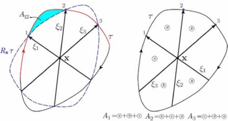
Figure 7: Stationary chords near to long-chord catastrophe of the Wigner function, displaying the compositions of the area $A_{j}$ for each stationary chord. The phase difference for coalescent $\mbox{\boldmath$\xi$}_{1}$ and $\mbox{\boldmath$\xi$}_{2}$ chords is the symplectic area $A_{12}$ limited by their tips.

so that, the Wigner function is given by

$$W({\mathbf{x}})=2\sqrt{2}N^{2}\left[\frac{\left[\frac{3}{4}A_{12}\right]^{\frac{1}{6}}\,\Sigma I_{12}\sin\left(\frac{\Sigma A}{2\mbox{\amsb\char 125\relax}}\right)}{\mbox{\amsb\char 125\relax}^{\frac{2}{3}}}{\rm Ai}\left(-\left[\frac{3A_{12}}{4\mbox{\amsb\char 125\relax}}\right]^{\frac{2}{3}}\right)\right.$$

$$\hskip 56.9055pt\left.-\frac{\Delta I_{12}\cos\left(\frac{\Sigma A}{2\mbox{\amsb\char 125\relax}}\right)}{\mbox{\amsb\char 125\relax}^{\frac{1}{3}}\left[\frac{3}{4}A_{12}\right]^{\frac{1}{6}}}{\rm Ai}^{\prime}\left(-\left[\frac{3A_{12}}{4\mbox{\amsb\char 125\relax}}\right]^{\frac{2}{3}}\right)\right]+W_{3}({\mathbf{x}}).$$ (45)

Again, as for chord function, the behaviour near the caustic is described correctly in terms of the Airy function and its derivative. The fact that the Wigner function also has cusps, which are of higher order than the catastrophes of the chord function, adds an additional term. Crossing the fold caustic, the coalescent chords disappear and only the additional term remains, coinciding with the simpler stationary phase approximation far form the causticBerry77 , although the normalization constant must be re-evaluated.

For regions where $A_{12}\gg\mbox{\amsb\char 125\relax}$, we can replace the Airy function and its derivative by their asymptotic forms for large negative values, obtaining

$$W({\mathbf{x}})=\frac{4N^{2}}{\sqrt{2\pi\mbox{\amsb\char 125\relax}}}\left[\frac{\sin\left(\frac{A_{1}}{\mbox{\amsb\char 125\relax}}-\frac{\pi}{4}\right)}{|\{I_{1}^{+},I_{1}^{-}\}|^{\frac{1}{2}}}+\frac{\sin\left(\frac{A_{2}}{\mbox{\amsb\char 125\relax}}+\frac{\pi}{4}\right)}{|\{I_{2}^{+},I_{2}^{-}\}|^{\frac{1}{2}}}+\frac{\cos\left(\frac{A_{3}}{\mbox{\amsb\char 125\relax}}-\frac{\pi}{4}\right)}{|\{I_{3}^{+},I_{3}^{-}\}|^{\frac{1}{2}}}\right]$$ (46)

which is a sum of oscillatory terms, each one with a different phase, as in (7). This asymptotic form is a superposition of the individual stationary phase approximations for each stationary chord.

V Approximations for the transitional regions

The uniform approximation (37) is not explicitly resolved very close to the caustic, because $\mathcal{A}_{12}\to 0$ as the caustic is approached, whereas $\Sigma I^{12}\to\infty$. The classical curve can be approximated by parabolae in both the neighborhoods of the tips of the realization of $\mbox{\boldmath$\xi$}_{D}$. This equates the amplitude associated for each stationary point, i.e. $\Sigma I^{12}=2\{I^{+},I^{-}\}$ and $\Delta I^{12}\to 0$. Thus, the term of the derivative of the Airy function in (37) cancels near to the caustic.

To obtain an explicit expression for the transitional chord function, we start by recalling that the action variable, $I({\mathbf{x}})$, can be interpreted as a Hamiltonian, such that the classical curve is a trajectory, i.e. the level curve $I({\mathbf{x}})=\mathcal{I}$. Considering ${\mathbf{x}}$ as the centre of a chord $\eta$ that conects two points of the curve, ${\mathbf{x}}_{a}$ and ${\mathbf{x}}_{b}$, we obtain as a first approximation, ${\mathbf{x}}_{b}\simeq{\mathbf{x}}_{a}+\tau\dot{{\mathbf{x}}}_{a}$, if ${\mathbf{x}}$ is very close to this curve. Then the action can be expanded as (see Appendix B in Ref. OzorioRep )

$$\mathcal{I}-I({\mathbf{x}})\simeq\frac{1}{8}\tau^{2}\,\dot{\mathbf{x}}\,\mathfrak{I}_{\mathbf{x}}\,\dot{\mathbf{x}},$$ (47)

where $\mathfrak{I}_{\mathbf{x}}$ is the Hessian matrix of $I$ at the point ${\mathbf{x}}$. This quadratic Hamiltonian generates the assumed linear motion. On the other hand, the area between $\eta$ and the curve (Fig. 8)

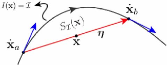
Figure 8: The area $S_{\mathcal{I}}$ for a point very close to the level curve, $I({\mathbf{x}})=\mathcal{I}$. The tips of the chord $\eta$ evolve by the action of the Hamiltonian $I({\mathbf{x}})$. As a first approximation, this evolution is linear.

is given by OzorioRep .

$$S_{\mathcal{I}}({\mathbf{x}})\simeq\frac{1}{12}\tau^{3}\,\dot{\mathbf{x}}\,\mathfrak{I}_{\mathbf{x}}\,\dot{\mathbf{x}}.$$ (48)

Thus, noticing that the centres of the realizations of $\eta$ are ${\mathbf{X}}^{\pm}\equiv\pm\mbox{\boldmath$\xi$}/2$, the symplectic area $\mathcal{A}_{12}$ in Fig. 5 may be obtained as

$$\mathcal{A}_{12}(\mbox{\boldmath$\xi$})=S_{\mathcal{I}}(\mbox{\boldmath$\xi$}/2)+S_{\mathcal{I}}(-\mbox{\boldmath$\xi$}/2)=\frac{1}{12}\left(\tau_{+}^{3}\dot{{\mathbf{X}}}^{+}\mathfrak{I}_{\frac{\bm{\xi}}{2}}\dot{{\mathbf{X}}}^{+}+\tau_{-}^{3}\dot{{\mathbf{X}}}^{-}\mathfrak{I}_{\scalebox{1.0}{-}\frac{\bm{\xi}}{2}}\dot{{\mathbf{X}}}^{-}\right)$$ (49)

where $\tau_{\pm}$ is the time of flight between the tips of each realization of $\eta$, under the action of the Hamiltonian $I({\mathbf{x}})$.

Recalling that ${\mathbf{x}}_{1}$ and ${\mathbf{x}}_{2}$ are the midpoints of the realizations of $\xi$, the Poisson brackets of the action in the amplitudes in (37) will be given by the symplectic products,

$$\dot{\mathbf{x}}_{1}^{+}\wedge\dot{\mathbf{x}}_{1}^{-}=\{I_{1}^{+},I_{1}^{-}\}\simeq-\{I_{2}^{+},I_{2}^{-}\}=\dot{\mathbf{x}}_{2}^{-}\wedge\dot{\mathbf{x}}_{2}^{+}$$ (50)

So that defining the ‘accelerations’OzorioRep ; Berry89 , $\ddot{\mathbf{x}}_{1}$ and $\ddot{\mathbf{x}}_{2}$, as

$$\ddot{\mathbf{x}}_{j}=\left(\dot{\mathbf{x}}_{j}\cdot\frac{\partial}{\partial{\mathbf{x}}}\right)\dot{\mathbf{x}}={\mathbf{J}}\mathfrak{I}_{\mathbf{x}}\dot{\mathbf{x}},$$ (51)

such that $\dot{\mathbf{x}}_{2}^{+}\simeq\dot{\mathbf{x}}_{1}^{+}+\tau_{+}\ddot{\mathbf{x}}_{1}^{+}$ and $\dot{\mathbf{x}}_{1}^{-}\simeq\dot{\mathbf{x}}_{2}^{-}+\tau_{-}\ddot{\mathbf{x}}_{2}^{-}$, we obtain

$$\{I_{1}^{+},I_{1}^{-}\}=\frac{1}{2}\left[\tau_{+}\dot{\mathbf{X}}^{-}\mathfrak{I}_{\frac{\xi}{2}}\dot{\mathbf{X}}^{+}+\tau_{-}\dot{\mathbf{X}}^{+}\mathfrak{I}_{\scalebox{1.0}{-}\frac{\xi}{2}}\dot{\mathbf{X}}^{-}\right]$$ (52)

The times $\tau_{+}$ and $\tau_{-}$ can be found using (47), so that (49) becomes

$$\frac{3}{4}\mathcal{A}_{12}(\mbox{\boldmath$\xi$})=\sqrt{2}\left[\frac{[\mathcal{I}-I(\frac{\bm{\xi}}{2})]^{\frac{3}{2}}}{[\dot{\mathbf{X}}^{+}\mathfrak{I}_{\frac{\bm{\xi}}{2}}\dot{\mathbf{X}}^{+}]^{\frac{1}{2}}}+\frac{[\mathcal{I}-I(\scalebox{1.0}{-}\frac{\bm{\xi}}{2})]^{\frac{3}{2}}}{[\dot{\mathbf{X}}^{-}\mathfrak{I}_{\scalebox{1.0}{-}\frac{\bm{\xi}}{2}}\dot{\mathbf{X}}^{-}]^{\frac{1}{2}}}\right].$$ (53)

Thus, we have all the necessary ingredients to obtain the transitional form of the chord function,

$$\chi(\mbox{\boldmath$\xi$}) = \frac{e^{i\Sigma\mathcal{A}/2\mbox{\amsb\char 125\relax}-i\pi/2}}{\pi^{\frac{1}{3}}h^{\frac{2}{3}}}\frac{[\tau_{+}^{3}\dot{\mathbf{X}}^{+}\mathfrak{I}_{\frac{\bm{\xi}}{2}}\dot{\mathbf{X}}^{+}+\tau_{-}^{3}\dot{\mathbf{X}}^{-}\mathfrak{I}_{\scalebox{1.0}{-}\frac{\bm{\xi}}{2}}\dot{\mathbf{X}}^{-}]^{\frac{1}{6}}}{[\tau_{+}\dot{\mathbf{X}}^{-}\mathfrak{I}_{\frac{\bm{\xi}}{2}}\dot{\mathbf{X}}^{+}+\tau_{-}\dot{\mathbf{X}}^{+}\mathfrak{I}_{\scalebox{1.0}{-}\frac{\bm{\xi}}{2}}\dot{\mathbf{X}}^{-}]^{\frac{1}{2}}}$$ (54)

$$\hskip 71.13188pt\times{\rm Ai}\left(-2^{\frac{1}{3}}\left[\frac{[\mathcal{I}-I(\frac{\bm{\xi}}{2})]^{\frac{3}{2}}}{[\dot{\mathbf{X}}^{+}\mathfrak{I}_{\frac{\bm{\xi}}{2}}\dot{\mathbf{X}}^{+}]^{\frac{1}{2}}}+\frac{[\mathcal{I}-I({\scalebox{1.0}{-}\frac{\bm{\xi}}{2}})]^{\frac{3}{2}}}{[\dot{\mathbf{X}}^{-}\mathfrak{I}_{\scalebox{1.0}{-}\frac{\bm{\xi}}{2}}\dot{\mathbf{X}}^{-}]^{\frac{1}{2}}}\right]^{\frac{2}{3}}\right).$$

If the curve has a local symmetry of reflection with respect to the origin, the hessian matrices will be equal, i.e. $\mathfrak{I}_{\frac{\bm{\xi}}{2}}=\mathfrak{I}_{\scalebox{1.0}{-}\frac{\bm{\xi}}{2}}$ and the velocity vectors $\dot{\mathbf{X}}^{+}=-\dot{\mathbf{X}}^{-}$. Here we recall that the origin depends of the chord $\xi$, since it has been chosen to be the midpoint between the centres of its realizations on the closed curve. Thus, the transitional chord function reduces in this simple case to

$$\chi(\mbox{\boldmath$\xi$})=\frac{e^{i\Sigma\mathcal{A}/2\mbox{\amsb\char 125\relax}+i\pi}}{(2\pi)^{\frac{1}{3}}h^{\frac{2}{3}}}[\dot{\mathbf{X}}^{+}\mathfrak{I}_{\frac{\bm{\xi}}{2}}\dot{\mathbf{X}}^{+}]^{-\frac{1}{3}}{\rm Ai}\left(2\frac{I(\frac{\bm{\xi}}{2})-\mathcal{I}}{[\dot{\mathbf{X}}^{+}\mathfrak{I}_{\frac{\bm{\xi}}{2}}\dot{\mathbf{X}}^{+}]^{\frac{1}{3}}}\right).$$ (55)

For a diameter $\mbox{\boldmath$\xi$}_{D}$, the argument of the Airy function cancels, because $I(\pm\mbox{\boldmath$\xi$}_{D}/2)=\mathcal{I}$, and $\Sigma\mathcal{A}/2$ is the chord area of $\mbox{\boldmath$\xi$}_{D}$. Thus, the transitional approximation remains finite, and at the caustic it is close to a local amplitude maximum.

We can follow a similar procedure for the Wigner function. Defining $\bar{\mbox{\boldmath$\xi$}}$, as the average between the stationary chords $\mbox{\boldmath$\xi$}_{1}$ and $\mbox{\boldmath$\xi$}_{2}$, together with the pair of phase space points, $\bm{y}^{\pm}={\mathbf{x}}\pm\bar{\mbox{\boldmath$\xi$}}/2$, we obtain

$$W(\mbox{\boldmath$\xi$}) = \frac{4\sin\left[\frac{\Sigma\mathcal{A}}{2\mbox{\amsb\char 125\relax}}\right]}{\pi^{\frac{1}{3}}h^{\frac{2}{3}}}\frac{[\tau_{+}^{3}\dot{\bm{y}}^{+}\mathfrak{I}_{{\bm{y}}^{+}}\dot{\bm{y}}^{+}-\tau_{-}^{3}\dot{\bm{y}}^{-}\mathfrak{I}_{{\bm{y}}^{-}}\dot{\bm{y}}^{-}]^{\frac{1}{6}}}{[\tau_{-}\dot{\bm{y}}^{+}\mathfrak{I}_{{\bm{y}}^{-}}\dot{\bm{y}}^{-}-\tau_{+}\dot{\bm{y}}^{-}\mathfrak{I}_{{\bm{y}}^{+}}\dot{\bm{y}}^{+}]^{\frac{1}{2}}}$$ (56)

$$\hskip 71.13188pt\times{\rm Ai}\left(-2^{\frac{1}{3}}\left[\frac{[\mathcal{I}-I(\bm{y}^{+})]^{\frac{3}{2}}}{[\dot{\bm{y}}^{+}\mathfrak{I}_{\bm{y}^{+}}\dot{\bm{y}}^{+}]^{\frac{1}{2}}}-\frac{[\mathcal{I}-I(\bm{y}^{-})]^{\frac{3}{2}}}{[\dot{\bm{y}}^{-}\mathfrak{I}_{\bm{y}^{-}}\dot{\bm{y}}^{-}]^{\frac{1}{2}}}\right]^{\frac{2}{3}}\right).$$

Unlike the chord function, this transitional form is undetermined at the caustic, in the particular case that the state is invariant with respect to a reflection symmetry, because then the entire caustic colapses to a point, where the Wigner function has a catastrophe of higher order.

VI Long-chord regime for Fock states

Now we consider the excited states, $|n\rangle$, of the one dimensional harmonic oscillator whose classical manifold is a circumference centred at the origin, i.e. it has reflection symmetry. The quantization condition (14) for these circles defines

$$\pi(p^{2}+q^{2})=2\pi\mbox{\amsb\char 125\relax}\left(n+\frac{1}{2}\right).$$ (57)

The exact chord function is given by OzVaSa

$$\chi_{n}(\xi)=\frac{e^{-\xi^{2}/4\mbox{\amsb\char 125\relax}}}{2\pi\mbox{\amsb\char 125\relax}}L_{n}\left(\frac{\xi^{2}}{2\mbox{\amsb\char 125\relax}}\right),$$ (58)

where $L_{n}$ is a Laguerre polynomial. For small chords, $\xi\ll\mbox{\amsb\char 125\relax}$,

$$\chi_{\mathcal{I}}(\xi)\simeq\frac{1}{2\pi\mbox{\amsb\char 125\relax}}J_{0}\left(\frac{\sqrt{2\mathcal{I}}|\xi|}{\mbox{\amsb\char 125\relax}}\right),$$ (59)

gives a good approximation for the chord function OzVaSa , where $J_{0}$, is the Bessel function of order zero. Then, the asymptotic form of the Bessel function for large values abramowitz leads to

$$\chi_{\mathcal{I}}(\xi)\simeq\frac{(\sqrt{2\mathcal{I}}|\xi|)^{-\frac{1}{2}}}{\pi\sqrt{h}}\cos\left(\frac{\sqrt{2\mathcal{I}}|\xi|}{\mbox{\amsb\char 125\relax}}-\frac{3\pi}{4}\right).$$ (60)

We can compare this result with the oscillatory regime (39). First, due to symmetry, the area of one chord realization is complementary to the area of the other and a simple integral gives the semiclassical phase as

$$\mathcal{A_{I}}(\xi)=2\pi\mathcal{I}-|\xi|\sqrt{2\mathcal{I}-\left(\frac{|\xi|}{2}\right)^{2}}-4\mathcal{I}\arcsin\left(\frac{|\xi|/2}{\sqrt{2\mathcal{I}}}\right).$$ (61)

Moreover, symmetry equates the Poisson bracket for each chord realization, so that terms containing the derivative of Airy function will cancel. The Poisson brackets are then evaluated as

$$\{I^{+},I^{-}\}=|\xi|\sqrt{2\mathcal{I}-\left(\frac{|\xi|}{2}\right)^{2}},$$ (62)

so that, the uniform approximation for the chord function becomes

$$\chi_{\mathcal{I}}(\xi)=(-1)^{n}\frac{\sqrt{2}N^{2}\left[\frac{3}{4}\mathcal{A_{I}}(\xi)\right]^{\frac{1}{6}}}{\mbox{\amsb\char 125\relax}^{\frac{2}{3}}|\xi|^{\frac{1}{2}}}\left[2\mathcal{I}-\frac{|\xi|^{2}}{4}\right]^{-\frac{1}{4}}{\rm Ai}\left(-\left[\frac{3\mathcal{A_{I}}}{4\mbox{\amsb\char 125\relax}}\right]^{\frac{2}{3}}\right).$$ (63)

It follows that the asymptotic behaviour of Airy function, extrapolated for small chords is

$$\chi_{\mathcal{I}}(\xi)=(-1)^{n}\frac{2N^{2}}{\sqrt{h}}\left(\sqrt{2\mathcal{I}}|\xi|\right)^{-\frac{1}{2}}\cos\left(\frac{\mathcal{A_{I}}}{2\mbox{\amsb\char 125\relax}}-\frac{\pi}{4}\right).$$ (64)

Note that, to lowest order, the argument in the Bessel function (59), $\sqrt{2\mathcal{I}}|\xi|$, is one half of the complementary area to the intersection between the circle and its translation.

Thus, the asymptotic limit of the chord function for the long-chord caustic reproduces the chord function of small chords for Fock states, in an intermediary region. Furthermore, we immediately obtain the normalization constant as

$$N^{2}=\frac{1}{2\pi}.$$ (65)

This is an alternative derivation to Berry’s Berry77 . We can replace this value in (46) outside the caustic, where the two coalescent chords disappear, so as to recover the simpler stationary phase approximation for the Wigner function Berry77 .

VII Discussion

We have shown that the behaviour of both the Wigner function and the chord function near a maximal chord singularity can be described by the Airy function and its derivative. Although, the latter becomes negligible for points very close to the caustic, it adds an important contribution to the expansion of the semiclassical distributions in the oscillatory region, coinciding there with the simpler stationary phase method. The shape of the diameter-caustic is different in the phase space of centres, ${\mathbf{x}}$, where the Wigner function is defined, and in the space of chords, $\xi$. In the latter case, the caustic is located on the locus of diameters, $\mbox{\boldmath$\xi$}_{D}$, maximal chords of the original closed complex curve. This diameter caustic is symmetrical with respect to the chord origin and it is also convex. If the assumption of convexity is relaxed, the symmetry will be preserved, because $-\mbox{\boldmath$\xi$}_{D}$ is also a diameter, but the simple fold caustic may then exhibit higher singularities. This is the case for the diameter-caustic viewed in the phase space of centres ${\mathbf{x}}_{D}={\mathbf{x}}(\mbox{\boldmath$\xi$}_{D})$. This caustic of the Wigner function has cusps even in the case of a convex quantized curve Berry77 .

The pair of caustics that concern us may be viewed as alternative projection singularities of a single (lagrangian) surface in a doubled phase space, ${\mathbf{X}}={\mathbf{x}}^{-}\times{\mathbf{x}}^{+}$, i.e the product torus for the pair of quantized curves $I({\mathbf{x}}^{\pm})=\cal{I}$. The alternative description of double phase space in terms of the centres, ${\mathbf{x}}=({\mathbf{x}}^{+}+{\mathbf{x}}^{-})/2$ and $\mbox{\boldmath$\xi$}=\mbox{\boldmath$\xi$}^{+}-\mbox{\boldmath$\xi$}^{-}$ leads to a description of the double torus that no longer factors Oz-enta . The points ${\mathbf{X}}_{D}=({\mathbf{x}}(\mbox{\boldmath$\xi$}_{D}),\mbox{\boldmath$\xi$}_{D})$ on the double torus project singularly onto both these double phase space coordinate planes. Thus the two-dimensional tangent plane to the torus is completely determined by the pair of tangent vectors: $({\mathbf{x}}(\mbox{\boldmath$\xi$}_{D}),0)$ and $(0,\mbox{\boldmath$\xi$}_{D})$.

Let us summarize the behaviour of the chord function for any translation: $a)$ a maximum at the origin; $b)$ an oscillatory regime, obtained as a superposition of stationary phase terms for each chord realization; $c)$ a region near to the maximal chord, i.e. the diameter $\mbox{\boldmath$\xi$}_{D}$, expressed in terms of the Airy function and its derivative, where the amplitude is again maximal and finally $d)$ an evanescent region for chords longer than diameters (also described by the Airy functions).

We have considered only pure states, for which the phase space correlation (5) is given by the square modulus of the chord function. Thus, using the asymptotic form of the uniform approximation for the chord function at the semiclassical regime, we find that, in the oscillatory region far from the caustic, the phase space correlation is approximately

$$C_{\xi}=\frac{1}{\mbox{\amsb\char 125\relax}}\left[\{I_{1}^{+},I_{1}^{-}\}^{-1}+\{I_{2}^{+},I_{2}^{-}\}^{-1}+2\{I_{1}^{+},I_{1}^{-}\}^{-\frac{1}{2}}\{I_{2}^{+},I_{2}^{-}\}^{-\frac{1}{2}}\sin\left(\frac{\mathcal{A}_{12}}{\mbox{\amsb\char 125\relax}}\right)\right],$$ (66)

i.e. a pair of classical terms associated to each chord realization and a term that represents their interference. This formula corrects the semiclassical phase space correlation presented in OzVaSa , which also provides a semiclassical interpretation for the invariance of the correlation with respect to Fourier transformation. The important point is that the maximal reach of the phase space correlations (also the correlations of the Wigner function) in the neighbourhood of a diameter of the quantized curve is just $C_{\xi}=|\chi(\mbox{\boldmath$\xi$})|^{2}$ in the simple form given by (55).

Appendix A Crossed chords

Redefining $S_{i}=S_{+}$ and $S_{j}=S_{-}$ in (17), the phase in the integrand for the Wigner function evaluated at the point ${\mathbf{x}}=(p,q)$ is

$$\mbox{\amsb\char 125\relax}F(Q;{\mathbf{x}})=S_{+}(q+Q/2,I)-S_{-}(q-Q/2)-pQ.$$ (67)

Let $q_{0}$ and $q_{1}$ be the turning points on the closed curve, with $q_{0}<q_{1}$. Choosing the $q$-axis to pass through $q_{0}$, according to Fig. 9, then at the stationary phase points, $Q=\pm\mbox{\boldmath$\xi$}_{q}$, we have

$$S_{+}(q+\xi_{q}/2) = \int_{q_{0}}^{q+{\xi_{q}}/2}p_{+}(Q)dQ=a_{1},$$ (68)

$$S_{-}(q-\xi_{q}/2) = \int_{q_{0}}^{q_{1}}p_{+}(Q)dQ+\int_{q_{1}}^{q-\xi_{q}/2}p_{-}(Q)dQ=a_{1}+a_{2}+a_{3}+[-a_{3}+a_{4}].$$ (69)

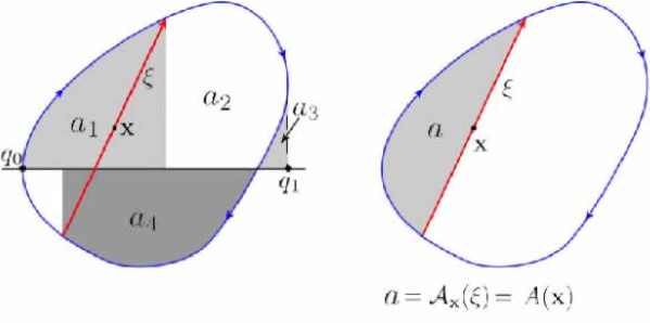
Figure 9: Phase difference between the stationary phase points for the Wigner function, evaluated at ${\mathbf{x}}=(p,q)$, such that the tips of its chord, $\xi=({\xi_{p}},{\xi_{q}})$, lie on different branches of the WKB function. The shaded area, $a=S_{+}(q+\xi_{q}/2)-S_{-}(q-{\xi_{q}}/2)-p{\xi_{q}}$,

The stationary chord, $\xi$, is here assumed to be crossed, i.e to have both its tips on different action branches. Then, the phase becomes

$$\mbox{\amsb\char 125\relax}F(\xi_{q};{\mathbf{x}})=a_{1}-[a_{1}+a_{2}+a_{4}]-p{\xi_{q}}=-[a_{2}+a_{4}]-p{\xi_{q}}=a-\oint pdq.$$ (70)

Defining $A({\mathbf{x}})$ as the area between the stationary chord and the closed curve, leads to

$$\mbox{\amsb\char 125\relax}F(\xi_{q};{\mathbf{x}})=A({\mathbf{x}})-\oint pdq=A({\mathbf{x}})-2\pi\left(n+\frac{1}{2}\right).$$ (71)

On the other hand, the phase of the integrand in (24) that defines the chord function for the same geometry is

$$\mbox{\amsb\char 125\relax}F_{\chi}(Q,\xi)=S_{+}(Q+\xi_{q}/2)-S_{-}(Q-\xi_{q}/2)-\xi_{p}Q.$$ (72)

The stationary points are position coordinates $q$, but their geometrical interpretation provides the respective momentum coordinates, $p$ (as discussed in sec. 2). Again we denote ${\mathbf{x}}=(p,q)$, thus the stationary phase $F_{\chi}$ depends of ${\mathbf{x}}$ instead of only $q$. Choosing the $q$-axis in the same way as before, we obtain

$$\mbox{\amsb\char 125\relax}F_{\chi}({\mathbf{x}},\xi) =S_{+}(q+\xi_{q}/2)-S_{-}(q-\xi_{q}/2)-p{\xi_{q}}+p{\xi_{q}}-\xi_{p}q,$$ (73)

$$=S_{+}(q+\xi_{q}/2)-S_{-}(q-\xi_{q}/2)-p{\xi_{q}}+{\mathbf{x}}\wedge\xi$$ (74)

Defining $\mathcal{A}_{\mathbf{x}}(\xi)$ as the symplectic area between the closed curve and the realization of $\xi$, centred on ${\mathbf{x}}$, as in Fig. 9, leads to

$$\mbox{\amsb\char 125\relax}F_{\chi}({\mathbf{x}},\xi)=\mathcal{A}_{\mathbf{x}}(\xi)+{\mathbf{x}}\wedge\xi-2\pi\left(n+\frac{1}{2}\right).$$ (75)

In order to implement the uniform approximations in sec. 3 and 4, we can ignore the additional term $\oint pdq$ in (71) and (75), because it is quantized. It should be recalled that the quantization of the closed curve implies that the areas, $A({\mathbf{x}})$ and $\mathcal{A}_{\mathbf{x}}(\xi)$ and their respective complementary areas, $A^{\prime}({\mathbf{x}})$ e $\mathcal{A}_{\mathbf{x}}^{\prime}(\xi)$, satisfy the rule

$$A({\mathbf{x}})+A^{\prime}({\mathbf{x}})=\mathcal{A}_{\mathbf{x}}(\xi)+\mathcal{A}_{\mathbf{x}}^{\prime}(\xi)=\oint p\,dq=2\pi\mbox{\amsb\char 125\relax}\left(n+\frac{1}{2}\right),\quad\quad\quad n\in\mathbb{Z}.$$ (76)

References

(1) Wigner E P Phys. Rev. 40 749
(2) Berry M V,
Phil. Trans. R. Soc. Lond. , 30
(1977)
(3) Leonhardt U,
Measuring the Quantum State of Light (Cambrigde: Cambridge University Press)
(1997)
(4) Ozorio de Almeida A M,
Phys. Rep. 265
(1998)
(5) Chountasis S and Vourdas A
Phys. Rev. A. 3, pp 1794
(1998)
(6) Royer A 1977
Phys. Rev. A15 449
(7) Ozorio de Almeida A M , Vallejos R O and Saraceno M,
J. Phys. A: Math. Gen., , 1473-1490
(2005)
(8) Ozorio de Almeida A M,
Entanglement in phase space,
eprintarXiv:quant-ph/0612029
(2006)
(To be published in Theoretical Foundations of Quantum Information,
edited by Buchleitner A and Viviescas C (Lecture Notes in Physics:Springer, Berlin))
(9) Van Vleck J H,
Proc. Math. Acad. Sci. U.S.A , 178 - 188
(1928)
(10) Maslov V P and Fedoriuk M V
Semiclassical Approximation in Quantum Mechanics(Reidel, Dordrecht)
(1981) (translated from original russian edition, 1965).
(11) Ozorio de Almeida A M,
Hamiltonian Systems: Chaos and Quantization (Cambrigde: Cambridge University Press)
(1988)
(12) Gutzwiller M,
Chaos in Classical and Quantum Mechanics (Springer, New York)
(1990)
(13) Chester C, Friedman B and Ursell F,
Proc. Camb. Phil. Soc. Math. Phys. Sci. , 599
(1957)