A Prototype Large-Angle Photon Veto Detector
for the P326 Experiment at CERN

Abstract

The P326 experiment at the CERN SPS has been proposed with the purpose of measuring the branching ratio for the decay $K^{+}\to\pi^{+}\nu\bar{\nu}$ to within $\sim$10%. The photon veto system must provide a rejection factor of $\mbox{10}^{\mbox{\scriptsize{8}}}$ for $\pi^{0}$ decays. We have explored two designs for the large-angle veto detectors, one based on scintillating tiles and the other using scintillating fibers. We have constructed a prototype module based on the fiber solution and evaluated its performance using low-energy electron beams from the Frascati Beam-Test Facility. For comparison, we have also tested a tile prototype constructed for the CKM experiment, as well as lead-glass modules from the OPAL electromagnetic barrel calorimeter. We present results on the linearity, energy resolution, and time resolution obtained with the fiber prototype, and compare the detection efficiency for electrons obtained with all three instruments.

I The P326 Experiment

THE branching ratio (BR) for the decay $K^{+}\to\pi^{+}\nu\bar{\nu}$ can be related to the value of the CKM matrix element $V_{td}$ with minimal theoretical uncertainty, providing a sensitive probe of the flavor sector of the Standard Model. The measured value of the BR is $\mbox{1.47}^{+\mbox{\scriptsize{1.30}}}_{-\mbox{\scriptsize{0.89}}}\times\mbox{10}^{-\mbox{\scriptsize{10}}}$ on the basis of three detected events [1]. P326, an experiment at the CERN SPS, has been proposed with the goal of detecting $\sim$100 $K^{+}\to\pi^{+}\nu\bar{\nu}$ decays with a S/B ratio of 10:1 [2]. The experimental layout is illustrated in Fig. 1.

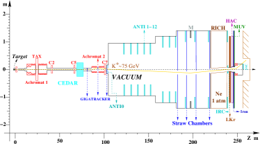
Figure 1: The P326 experimental layout.

The experiment will make use of a 75 GeV unseparated positive secondary beam. The total beam rate is 800 MHz, providing $\sim$50 MHz of $K^{+}$’s. The decay volume begins 102 m downstream of the production target. 10 MHz of kaon decays are observed in the 120-m long vacuum decay region. Large-angle photon vetoes are placed at 12 stations along the decay region and provide full coverage for decay photons with $\mbox{8.5~{}mrad}<\theta<\mbox{50~{}mrad}$. The last 35 m of the decay region hosts a dipole spectrometer with four straw-tracker stations operated in vacuum. The NA48 liquid-krypton calorimeter [3] is used to veto high-energy photons at small angle. Additional detectors further downstream extend the coverage of the photon veto system (e.g. for particles traveling in the beam pipe).

The experiment must be able to reject background from, e.g., $K^{+}\to\pi^{+}\pi^{0}$ decays at the level of $\mbox{10}^{\mbox{\scriptsize{12}}}$. Kinematic cuts on the $K^{+}$ and $\pi^{+}$ tracks provide a factor of $\mbox{10}^{\mbox{\scriptsize{4}}}$ and ensure 40 GeV of electromagnetic energy in the photon vetoes; this energy must then be detected with an inefficiency of $\geq\mbox{10}^{-\mbox{\scriptsize{8}}}$. For the large-angle photon vetoes, the maximum tolerable detection inefficiency for photons with energies as low as 200 MeV is $\mbox{10}^{-\mbox{\scriptsize{4}}}$. In addition, the large-angle vetoes must have good energy and time resolution and must be compatible with operation in vacuum.

II Large-Angle Photon Vetoes

The detectors at each veto station are ring shaped. The detectors at the first five veto stations have inner radii of 60 cm and outer radii of 96 cm. Those at the remaining stations have inner and outer radii to match the taper of the vacuum chamber; the largest covers $\mbox{90~{}cm}<r<\mbox{140~{}cm}$.

For the construction of the detectors themselves, two designs are under consideration. One consists of a sandwich of lead sheets and scintillating tiles with WLS-fiber readout. An assembly of wedge-shaped modules forms the veto station. An example of such a detector, using 80 layers of 1-mm thick lead sheets and 5-mm thick scintillating tiles, was designed for the (now canceled) CKM experiment at Fermilab. Tests of a prototype at Jefferson Lab showed that the inefficiency of the detector for 1.2 GeV electrons was at most $\mbox{3}\times\mbox{10}^{-\mbox{\scriptsize{6}}}$ [4].

An alternative solution is based on the design of the KLOE calorimeter [5], and consists of 1-mm diameter scintillating fibers sandwiched between 0.5-mm thick lead foils. The fibers are arranged orthogonal to the direction of particle incidence and are read out at both ends. Two U-shaped modules form a veto station. This solution offers advantages in terms of hermeticity, position resolution, and time resolution. Since a prototype based on the tile design has already been tested, we have opted to construct and test a prototype fiber module. We have obtained the CKM prototype on loan for further testing and comparison.

The remainder of this paper describes the construction of the fiber prototype and its testing with low-energy electron beams at the Frascati Beam-Test Facility (BTF). For the purposes of comparison, we also present preliminary results on the detection efficiency for low-energy electrons for the CKM tile prototype, and for lead-glass blocks from the OPAL electromagnetic barrel calorimeter.

III Construction of the Fiber Prototype

One U-shaped module was constructed at Frascati in fall 2006 (Fig. 2).

Figure 2: Schematic diagram of the fiber prototype attached to construction saddle.

The inner radius (60 cm) and length (310 cm along the inner face) of the prototype are identical to the specified values for one of the upstream veto stations in the actual experiment. The prototype has a radial thickness of 12.5 cm, corresponding to 35% of the specified value for one of the upstream stations. This thickness was chosen to reduce prototyping costs; it should be sufficient for transverse containment of low-energy electron showers incident half-way between the inner and outer edges of the module.

The materials used in construction were 0.5-mm thick lead foils from an industrial supplier, cut to $\mbox{350}\times\mbox{25~{}cm}^{\mbox{\scriptsize{2}}}$; 1-mm diameter Kuraray SCSF-81 scintillating fibers cut to 350 cm in length; and Bicron BC-600 optical cement. Layers of the module were constructed by rolling 1-mm grooves on 1.35-mm centers into the lead foils, and gluing scintillating fibers into the grooves. The 25-cm width of the lead foils determines the longitudinal depth of the module. The desired radial thickness was obtained by stacking 99 layers. The ends of the module were then milled and fitted with $\mbox{4.2}\times\mbox{4.2~{}cm}^{\mbox{\scriptsize{2}}}$ lucite light guides terminating in Winston-cone concentrators. This determines the segmentation of the module in the plane transverse to the fibers—there are three readout cells in the radial direction and six cells in depth. Light from the fibers is read-out by Hamamatsu R6427 28-mm photomultiplier tubes (PMTs) coupled to the light guides with optical grease.

In the region covered by the first four cells in depth, every groove in the lead is occupied by a scintillating fiber. In the region covered by the last two cells, the scintillating fibers in alternating grooves are replaced by lead wire. This reduces the number of scintillating fibers by 17% and increases the thickness of the module in radiation lengths.

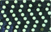
Figure 3: Photographs of fiber fill patterns in the (left) first four and (right) last two cells in longitudinal depth.

The resulting fill pattern is illustrated in Fig. 3. The first four cells in depth contain lead, fiber, and glue in the proportions 42:48:10 by volume, for a thickness of 13$X_{0}$. For the last two cells, the proportions are 66:24:10, for a thickness of 10$X_{0}$.

For construction of the prototype, we designed the steel and aluminum support structure, or “saddle,” seen in Fig. 2. The saddle also provides a convenient support structure for the completed module, allowing transportation and positioning during beam testing. However, the module is not structurally attached to the saddle. This was intended to allow experimentation at a later time with module mechanics and support structures for installation in the actual experiment. To avoid complications from nearby material for efficiency studies with beam incident near the inner face of the module, the saddle features a removable segment near its midpoint.

The module was constructed as follows. The lead foils were grooved using a rolling machine built for the construction of the KLOE calorimeter [5]. With the curved surface of the saddle upwards, a foil was draped over the saddle, the surface of the foil was painted with optical cement, and fibers were laid into the grooves. For the 16.8 cm in width corresponding to the first four readout cells in module depth, every groove is occupied by a fiber. In this region, the fibers were laid into the grooves en masse by simply distributing a counted number of fibers over the surface and smoothing them into place by hand. For the last two cells, fibers and lead wires were individually placed. The fibers were then painted with optical cement, and the next foil was draped on top, providing the bottom surface of the next layer. Four to six layers could be completed within the 2.5-hour pot life of the glue, after which time, a harmonic-steel band with threaded tensioning rods at either end was applied and tightened. Additional compression was provided by a series of clamps on the saddle. The module was left to set and cure overnight, and construction proceeded the following day.

When construction was complete and the module was instrumented as described above, the responses of the cells to minimum-ionizing particles were equalized to within 10–20% by adjusting the PMT voltages in successive cosmic-ray runs, in which the calorimeter was oriented with the U opening upward, and scintillator paddles were placed above and below the midpoint of the module.

IV Other Prototypes

As described in Sec. II, the prototype lead/scintillating-tile photon veto detector constructed for the CKM experiment was obtained on loan from Fermilab for testing and comparison. This detector is fully described in Ref. 4.

In addition, 3800 modules from the central part of the OPAL electromagnetic calorimeter barrel [6] have recently become available for use in P326. These modules consist of blocks of SF57 lead glass with an asymmetric, truncated square-pyramid shape. The front and rear faces of the blocks measure about $\mbox{10}\times\mbox{10~{}cm}^{\mbox{\scriptsize{2}}}$ and $\mbox{11}\times\mbox{11~{}cm}^{\mbox{\scriptsize{2}}}$, respectively; the blocks are 37 cm long. The modules are read out at the back side by Hamamatsu R2238 (76-mm diameter) PMTs, coupled via 4-cm cylindrical light guides of SF57. There are obvious practical advantages to basing the P326 large-angle photon veto system on existing hardware; the collaboration is actively seeking to understand whether these Cerenkov radiators are suitable. For most of our beam tests, we used a tower of four lead-glass blocks, with the beam centrally incident on the side face of the first module. In this configuration, the stack was $\sim$40 cm (27$X_{0}$) deep.

V The Frascati Beam-Test Facility

The Frascati BTF [7] is an electron transfer line leading off of the DA$\Phi$NE linac. The linac accelerates $e^{+}$’s and $e^{-}$’s to maximum energies of 550 and 800 MeV, respectively, producing 10-ns pulses with a repetition rate of 50 Hz. Momentum-selection magnets, attenuating targets, and collimation slits upstream of the experimental area can be used to produce test beams in the BTF hall with energies from $\sim$100 to 750 MeV with a 1% energy-selection resolution and mean multiplicities from $<$1 to $\mbox{10}^{\mbox{\scriptsize{9}}}$ per pulse.

The last magnet on the BTF line is a 45^∘ dipole with a hole in the yoke allowing extraction of a photon beam through an uncurved extension of the vacuum chamber. The apparatus for producing a tagged photon beam was developed for testing the AGILE satellite gamma-ray telescope [8]. A silicon microstrip beam tracker doubles as an active bremsstrahlung target upstream of the final dipole; silicon trackers inside the dipole gap register the trajectory of the electron after radiation, tagging the bremsstrahlung photon. While the tagged photon beam has been used with some success for energy calibration, e.g., of the AGILE satellite, at present, background levels in the photon beam are prohibitive for sensitive efficiency measurements. This background consists of photons from showering on upstream beam elements by particles from the attenuating target. Work is underway to improve the shielding around the attenuating target. In the meantime, we have used the electron beam to test the prototypes.

VI Readout and data acquisition

All prototypes were read out using the BTF front-end electronics and data acquisition (DAQ) system. For the fiber and tile prototypes, the PMT anode signals were passively split to obtain both charge and time measurements. For the lead-glass detectors, the signals were not split and only charge information was read out. CAEN V792 charge-to-digital converters (QDCs) were used for the charge measurements. CAEN V814 low-threshold discriminators and V775 time-to-digital converters (TDCs) were used for the time measurements. A signal from the linac gun provided QDC gates and TDC starts, as well as the DAQ trigger.

The 12-bit QDCs used reached full scale at 400 pC. A minimum-ionizing particle passing through the fiber prototype deposits 30 MeV per cell. For efficiency studies, we desired that this correspond to about 200 QDC counts. The HV settings obtained from calibration with cosmic rays as described in Sec. III then gave typical tube gains of $\mbox{1}\times\mbox{10}^{\mbox{\scriptsize{7}}}$.

VII Beam tagging system

The telescope of scintillation counters used to tag single-electron events

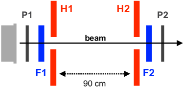
Figure 4: Schematic diagram of the beam tagging system, comprising two paddles for single-electron event selection (F1, F2), two hole counters for trajectory definition (H1, H2), and two beam-profile monitors for alignment (P1, P2).

is schematically illustrated in Fig. 4. From upstream to downstream, the following trigger counters, all made from 10-mm thick plastic scintillator, were used:

• a paddle of area $\mbox{60}\times\mbox{85}$ mm${}^{\mbox{\scriptsize{2}}}$, positioned a few centimeters downstream of the beamline exit window;

• a paddle of area $\mbox{200}\times\mbox{130}$ mm${}^{\mbox{\scriptsize{2}}}$ with a 14-mm diameter hole in the center, positioned $\sim$10 mm downstream of F1;

• a paddle of area $\mbox{330}\times\mbox{100}$ mm${}^{\mbox{\scriptsize{2}}}$ with a 14-mm diameter hole in the center, positioned 90 cm downstream of H1.

• a paddle of area $\mbox{60}\times\mbox{85}$ mm${}^{\mbox{\scriptsize{2}}}$, positioned $\sim$10 mm downstream of H2 and as little as 10 mm upstream of the prototype to be tested.

The tagging criterion for single-electron events used in the efficiency studies was $\mbox{F1}\cdot\overline{\mbox{H1}}\cdot\overline{\mbox{H2}}\cdot\mbox{F2}$, where F1 and F2 refer to charge signals on the paddle counters consistent with passage of a single electron, and $\overline{\mbox{H1}}$ and $\overline{\mbox{H2}}$ refer to null signals on the hole counters. Acceptable beam trajectories were thus defined by the two 14-mm diameter holes separated by 90 cm. The use of paddle/hole combinations rather than horizontal/vertical fingers was intended to reduce the amount of material in the beam. The fact that no material occupied the space between the hole counters was intended to facilitate alignment. The thickness of the paddles was chosen to allow efficient identification of events with exactly one electron in the paddles within the 10-ns linac pulse. The large dimensions of the hole counters served to help reject events with stray beam particles present. The use of a paddle (rather than a hole) as the last counter was intended to reduce mistags by providing a positive signal for beam particles just before entry into the prototype.

The mistag probability was monitored by taking occasional runs with the last dipole in the BTF beamline switched off, so that the beam was not directed towards the tagger or the prototypes. We did not find any tags in more than 1 million events collected in this configuration, corresponding to a false-tag rate of $<\mbox{2}\times\mbox{10}^{-\mbox{\scriptsize{6}}}$ at 90% CL. Based on our evaluation of the efficiencies for the F1 and F2 counters singly, we expect the contribution from false tags to be insignificant for the purposes of the efficiency measurements. In all cases, we quote efficiencies assuming no contribution from false tags. This assumption is conservative; if there are false tags, they artificially increase the inefficiency. The energy spectrum from the fiber prototype for fully-tagged events shows that, at most, multiple-electron events are present at the percent level (Fig. 8), and thus have a negligible effect on the normalization for the efficiency measurements.

The tagging system was mounted on a rigid support structure allowing fine and reproducible positioning of all counters in the horizontal and vertical coordinates. To facilitate alignment, the beam position in the bend plane was measured using the BTF beam-profile meters, which were mounted just upstream and downstream of the tagger (P1 and P2 in Fig. 4). Each profile meter is a one-dimensional, 16-channel close-packed array of 1-mm scintillating fibers read out by a multianode PMT, with each channel consisting of a group of fibers three across by four deep.

VIII Data Collection

The fiber prototype was first tested at the BTF during two-week runs in March and April 2007. During the April run, the tile prototype was also tested. These runs served primarily to debug the prototypes and optimize the tagging system.

TABLE I: Statistics Collected During the Summer 2007 BTF Run

	Beam energy [MeV]	$P(\mbox{1}e)$ [%]	$\varepsilon(\mbox{tag}|\mbox{1}e)$ [%]	Tagged events
Fiber prototype (KLOE)
	203	31.3	2.5	70k
	350	33.0	9.2	210k
	483	33.3	14.4	370k
Tile prototype (CKM)
	203	29.5	3.7	65k
	350	31.8	8.8	220k
	483	29.0	17.6	370k
Lead glass (OPAL)
	203	30.2	3.9	25k
	483	26.0	17.1	90k

The data analyzed for this report were collected during a 25-day run during June-July 2007. For the fiber and tile prototypes, data were taken at beam energies of 203, 350, and 483 MeV. For the lead-glass detectors, data were taken at beam energies of 203 and 483 MeV. Table I summarizes the data collected. For each instrument and point in beam energy, the total number of fully-tagged single-electron events is given, together with $P(\mbox{1}e)$, the probability for having an event of multiplicity one in the prototype (by Poisson statistics, $P(\mbox{1}e)=\mbox{36}$% in the best case), and $\varepsilon(\mbox{tag}|\mbox{1}e)$, the fraction of single-electron events in the prototype passing the full tagging criterion. There is a marked effect from multiple scattering in the tagger and in air: the tagging efficiency $\varepsilon(\mbox{tag}|\mbox{1}e)$ is significantly decreased at low energy.

In tests of the tile prototype at Jefferson Lab, data were taken at beam energies of 500, 800, and 1200 MeV. Our tests thus extend to significantly lower beam energies the experimental knowledge of the detection efficiency for this prototype.

In addition to the data samples listed in Table I, for each detector, smaller samples were also collected in a variety of configurations with the beam incident at different points and/or at different angles.

IX Results Obtained with the Fiber Prototype

IX-A Energy Reconstruction

We obtain separate energy measurements from the set of PMTs on each side of the prototype (sides A and B). We first subtract the mean noise level from the QDC measurements for each cell. The noise arises from diffuse background in the BTF hall; its mean level is determined from events with no activity in the tagger, and is typically larger than the sum of the hardware pedestals by an amount corresponding to a few MeV for the whole detector.

For each side, we take the energy measurement to be the gain-calibrated sum of the signals from all cells for which the uncalibrated QDC measurements are greater than the hardware pedestal by more than 3$\sigma$ (typically less than 10 counts, or $\sim$1.5 MeV). For the combined energy measurement from both sides, if there are signals above the 3$\sigma$ threshold from both PMTs, the energy measurement for the cell is the average of the measurements from each side. If instead one PMT gives a signal above threshold and the other does not, the energy measurement for the cell is equal to the measurement from the side above threshold.

For some runs with $E_{\mbox{\scriptsize{beam}}}=\mbox{350}$ and 500 MeV, a few of the QDC channels digitizing signals from side B of the prototype refused to register any counts above pedestal unless the integrated PMT signals exceeded the normal level of the hardware pedestal by $\sim$100 counts. This led to a loss of part of the signal from side B at low energies. When the energy measurements from both sides are combined, the use of the algorithm described above helps to recover the lost signal.

IX-B Linearity and Energy Resolution

Although seemingly a basic test of the prototype performance, the linearity of response is difficult to measure precisely with our setup. This is mainly because run-to-run fluctuations in the energy scale are observed at the $\sim$5% level. Several factors may contribute to such drifts, including limited reproducibility of the beam energy due to hysteresis in the BTF dipoles and possible time- (or temperature-) dependent drifts in HV power supply voltages or QDC gains. With additional effort during data taking, it should be possible to maintain better stability of the energy scale. In any event, for the energy resolution and efficiency measurements, we calibrate to a reference value of the energy for the single-electron peak, so these small drifts do not pose a problem. When testing the linearity, however, this calibration procedure cannot be applied at more than one energy point.

Figure 5: Response linearity for the fiber prototype. Top: $E_{\mbox{\scriptsize{meas}}}$ vs. $E_{\mbox{\scriptsize{beam}}}$ for $E_{\mbox{\scriptsize{beam}}}=\mbox{203}$, 350, and 483 MeV. Bottom: $(E_{\mbox{\scriptsize{meas}}}-E_{\mbox{\scriptsize{beam}}})/E_{\mbox{\scriptsize{beam}}}$ for each point.

In Fig. 5, we plot the measured mean value of the energy of the single-electron peak, $E_{\mbox{\scriptsize{meas}}}$, as a function of the beam energy, $E_{\mbox{\scriptsize{beam}}}$, where the energy scale has been fixed using the point at $E_{\mbox{\scriptsize{beam}}}=\mbox{203 MeV}$. $E_{\mbox{\scriptsize{meas}}}$ is obtained from Gaussian fits to the single-electron peak over an interval of about $\pm$1.5$\sigma$ about the peak. The lower panel of the figure shows the fractional deviation of $E_{\mbox{\scriptsize{meas}}}$ from $E_{\mbox{\scriptsize{beam}}}$. Such deviations are present at the level of $\sim$5%, i.e., at the level of precision with which the energy scale is known. (The errors on the plotted points include only the statistical measurement errors, plus a 1% systematic error corresponding to the BTF energy-selection resolution.)

We conclude that the response linearity is basically satisfactory. We do note that, in the actual experiment, multiple-range QDCs or some other readout scheme with extended dynamic range will be necessary, as full-scale is reached on the front cells for multiple-electron events in which the total energy deposit is $\sim$2 GeV.

Figure 6: Energy resolution for the fiber prototype at $E_{\mbox{\scriptsize{beam}}}=\mbox{203}$, 350, and 483 MeV.

To obtain the energy resolution, the Gaussian fits to the single-electron peak are performed again after the run-by-run energy scale calibration is applied. In Fig. 6, we plot the relative energy resolution, $\sigma_{E}/E_{\mbox{\scriptsize{meas}}}$, as a function of $E_{\mbox{\scriptsize{beam}}}$, for the measurements from each side of the prototype and for the combined measurement. The inferior performance of side B at $E_{\mbox{\scriptsize{beam}}}=\mbox{350}$ and 500 MeV is due to the loss of signal described in Sec. IX-A. The best performance is obtained by combining information from both sides. The curves in Fig. 6 show the results of fits to the form

$$\frac{\sigma_{E}}{E}=\frac{p_{\mbox{\scriptsize{1}}}}{\surd{E}\>\mbox{(GeV)}}\oplus p_{\mbox{\scriptsize{2}}}.$$

Using the information from both sides of the prototype, we find $p_{\mbox{\scriptsize{1}}}$ = 5.1% and $p_{\mbox{\scriptsize{2}}}$ = 4.4%. The coefficient obtained for the stochastic term ($p_{\mbox{\scriptsize{1}}}$) is in reasonable agreement with expectation from our preliminary Monte Carlo studies and from experience with the KLOE calorimeter.

IX-C Time resolution

In principle, the arrival time of a particle and its impact position along the length of the fibers would be obtained from the sum (average) and difference of the time measurements from the two sides of a cell. However, for the tests described here, the beam was incident at the midpoint of the fibers; we therefore have independent time measurements from each side of each cell. The time measurements for sides A and B, $t_{\mbox{\scriptsize{A}}}$ and $t_{\mbox{\scriptsize{B}}}$, and the combined time measurement $t_{\mbox{\scriptsize{A+B}}}$, are taken to be the energy-weighted averages of the time measurements for the corresponding group of cells. The event time reference is provided by the tagging system: $t_{\mbox{\scriptsize{tag}}}\equiv(t_{\mbox{\scriptsize{F1}}}+t_{\mbox{\scriptsize{F2}}})/\mbox{2}$, where F1 and F2 are the trigger paddles described in Sec. VII.

Slewing corrections and time offsets for each cell are obtained by fitting the time vs. QDC distributions with the form $t-t_{\mbox{\scriptsize{tag}}}\propto(\mbox{ln}\>Q_{0}/Q)^{\alpha}+t_{0}$, where $Q$ and $t$ are the QDC and time measurements, $t_{0}$ is the time offset for the cell, and $\alpha$ is positive. Slewing corrections are also necessary for $t_{\mbox{\scriptsize{F1}}}$ and $t_{\mbox{\scriptsize{F2}}}$, so an iterative procedure is applied.

Once all slewing corrections have been obtained, we form the distributions of the differences $t_{\mbox{\scriptsize{A}}}-t_{\mbox{\scriptsize{tag}}}$, $t_{\mbox{\scriptsize{B}}}-t_{\mbox{\scriptsize{tag}}}$, $t_{\mbox{\scriptsize{A}}}-t_{\mbox{\scriptsize{B}}}$, and $t_{\mbox{\scriptsize{F1}}}-t_{\mbox{\scriptsize{F2}}}$; fit with Gaussians; and from the four widths obtain $\sigma_{\mbox{\scriptsize{A}}}$, $\sigma_{\mbox{\scriptsize{B}}}$, $\sigma_{\mbox{\scriptsize{tag}}}$, and $\sigma_{\mbox{\scriptsize{AB}}}$, where this latter quantity accounts for common-mode fluctuations in the time measurements from the two sides ($\sigma_{\mbox{\scriptsize{AB}}}^{\mbox{\scriptsize{2}}}=2\,\mbox{cov}(t_{\mbox{\scriptsize{A}}},t_{\mbox{\scriptsize{B}}})$). The time resolution of the tagging system is found to be $\sigma_{\mbox{\scriptsize{tag}}}\approx\mbox{147 ps}$ and stable for points with different $E_{\mbox{\scriptsize{beam}}}$. We obtain the resolution on the combined time measurement for the two sides from the width of the distribution $t_{\mbox{\scriptsize{A+B}}}-t_{\mbox{\scriptsize{tag}}}$, with $\sigma_{\mbox{\scriptsize{tag}}}$ subtracted in quadrature.

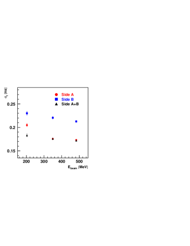
Figure 7: Time resolution for the fiber prototype at $E_{\mbox{\scriptsize{beam}}}=\mbox{203}$, 350, and 483 MeV (preliminary)

Our results on the time resolution are still preliminary. They are plotted in Fig. 7 as a function of $E_{\mbox{\scriptsize{beam}}}$. Again, the resolution is better on side A than it is on side B. For the point at 483 MeV, the resolution for the combined measurement is $\sigma_{\mbox{\scriptsize{A+B}}}=\mbox{172 ps}$, of which 158 ps is due to the common-mode fluctuation in the time measurements from each side. We do not yet fully understand the origin of this large contribution.

IX-D Efficiency

Our measurements of the detection efficiency are summarized in Fig. 8.

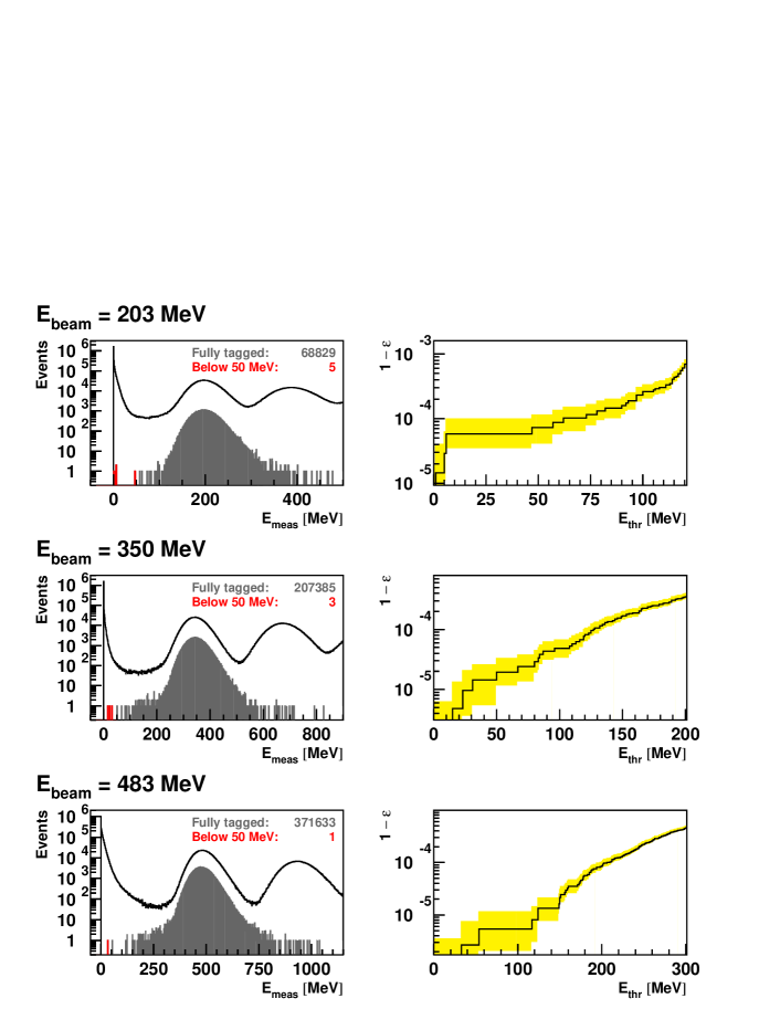
Figure 8: Measurements of detection efficiency for electrons with $E_{\mbox{\scriptsize{beam}}}=\mbox{203}$, 350, and 483 MeV. Left: Measured energy distributions for all events (open histograms) and for fully tagged events (shaded histograms). Right: Inefficiency as a function of $E_{\mbox{\scriptsize{thr}}}$.

For each beam energy, the panel on the left shows the energy distribution for all collected events (open histogram) and for fully-tagged events (shaded) histogram. The one- and two-electron peaks are clearly visible in the distribution for all events; application of the tagging criterion reduces the contribution from multiple-electron events to a level negligible for our purposes.

We consider a fully-tagged single-electron event to be undetected if the measured energy is below a threshold value of $E_{\mbox{\scriptsize{thr}}}=\mbox{50 MeV}$. At $E_{\mbox{\scriptsize{beam}}}=\mbox{203 MeV}$, we find five such events out of 68 829 total tagged events; at $E_{\mbox{\scriptsize{beam}}}=\mbox{350 MeV}$, we find three out of 207 385; and at 483 MeV, we find one out of 371 633. We thus quote inefficiencies of $\mbox{7.3}^{+\mbox{\scriptsize{4.1}}}_{-\mbox{\scriptsize{3.3}}}\times\mbox{10}^{-\mbox{\scriptsize{5}}}$, $\mbox{1.4}^{+\mbox{\scriptsize{1.1}}}_{-\mbox{\scriptsize{0.9}}}\times\mbox{10}^{-\mbox{\scriptsize{5}}}$, and $\mbox{2.7}^{+\mbox{\scriptsize{4.7}}}_{-\mbox{\scriptsize{1.7}}}\times\mbox{10}^{-\mbox{\scriptsize{6}}}$, respectively, where the asymmetric uncertainties represent 68.27% unified confidence intervals [9]. We assume that no undetected events are due to false tags.

The choice of threshold $E_{\mbox{\scriptsize{thr}}}=\mbox{50 MeV}$ is reasonable but arbitrary. For each beam energy, we obtain the inefficiency as a function of threshold from the normalized cumulative energy distribution for fully-tagged events. The results are presented in the right panels of Fig. 8. One again, the shaded bands indicate 68.27% unified confidence intervals, and we assume that there are no false tags. For $E_{\mbox{\scriptsize{beam}}}=\mbox{203 MeV}$, the inefficiency remains at the level of a few per mil even for thresholds as high as 100 MeV.

IX-E Comparison with Other Prototypes

The analysis of the data from the tile and lead-glass detectors is not yet complete, in particular with respect to the final, run-dependent energy calibrations.

TABLE II: Comparison of Detection Efficiencies for Three Prototypes

	Beam energy [MeV]	Tagged events	Tagged, $E_{\mbox{\scriptsize{meas}}}<\mbox{50 MeV}$	$\mbox{1}-\varepsilon$
Fiber prototype (KLOE)
	203	68 829	5	$\mbox{7.3}^{+\mbox{\scriptsize{4.1}}}_{-\mbox{\scriptsize{3.3}}}\times\mbox{10}^{-\mbox{\scriptsize{5}}}$
	350	207 385	3	$\mbox{1.4}^{+\mbox{\scriptsize{1.1}}}_{-\mbox{\scriptsize{0.9}}}\times\mbox{10}^{-\mbox{\scriptsize{5}}}$
	483	371 633	1	$\mbox{2.7}^{+\mbox{\scriptsize{4.7}}}_{-\mbox{\scriptsize{1.7}}}\times\mbox{10}^{-\mbox{\scriptsize{6}}}$
Tile prototype (CKM) - Preliminary
	203	65 165	2	$\mbox{3.1}^{+\mbox{\scriptsize{3.5}}}_{-\mbox{\scriptsize{1.9}}}\times\mbox{10}^{-\mbox{\scriptsize{5}}}$
	350	221 162	3	$\mbox{1.4}^{+\mbox{\scriptsize{1.0}}}_{-\mbox{\scriptsize{0.9}}}\times\mbox{10}^{-\mbox{\scriptsize{5}}}$
	483	192 412	1	$\mbox{5.2}^{+\mbox{\scriptsize{9.1}}}_{-\mbox{\scriptsize{3.3}}}\times\mbox{10}^{-\mbox{\scriptsize{6}}}$
Lead glass (OPAL) - Preliminary
	203	25 069	3	$\mbox{1.2}^{+\mbox{\scriptsize{0.9}}}_{-\mbox{\scriptsize{0.8}}}\times\mbox{10}^{-\mbox{\scriptsize{4}}}$
	483	91 511	1	$\mbox{1.1}^{+\mbox{\scriptsize{1.9}}}_{-\mbox{\scriptsize{0.7}}}\times\mbox{10}^{-\mbox{\scriptsize{5}}}$

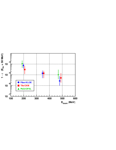
Figure 9: Comparison of detection efficiencies for each of the three prototypes, for 203, 350, and 483 MeV electrons with $E_{\mbox{\scriptsize{thr}}}=\mbox{50 MeV}$. Results obtained with the CKM tile prototype and OPAL lead-glass modules are preliminary.

Nevertheless, we believe that our preliminary results on the detection efficiencies for these prototypes are sufficiently stable to provide meaningful comparison with the results obtained with the fiber prototype. The results obtained for the inefficiency with $E_{\mbox{\scriptsize{thr}}}=\mbox{50 MeV}$ for all three prototypes are summarized in Table II and plotted in Fig. 9. The efficiency for detection of low-energy electrons is seen to be similar for all three technologies tested.

X Summary and Outlook

The large-angle photon veto detectors for the P326 experiment must have inefficiencies of less than $\mbox{10}^{-\mbox{\scriptsize{4}}}$ for the detection of photons with energies as low as 200 MeV. We have constructed a lead/scintillating-fiber prototype detector based on the KLOE calorimeter and tested it with electrons at the Frascati BTF. The performance of the prototype is in agreement with expectation; in particular, we obtain an energy resolution of $\sigma_{E}/E=\mbox{5.1\%}/\surd E\>\mbox{(GeV)}\oplus\mbox{4.4\%}$ and an inefficiency for the detection of 203 MeV electrons of $\mbox{7.3}^{+\mbox{\scriptsize{4.1}}}_{-\mbox{\scriptsize{3.3}}}\times\mbox{10}^{-\mbox{\scriptsize{5}}}$.

A preliminary analysis of data from the CKM tile prototype and from lead-glass modules from the OPAL barrel electromagnetic calorimeter suggests that all three detectors have similar detection efficiencies for electrons. However, the detection efficiency for photons may be worse, whether because of punch-through, or because of a high intrinsic inefficiency for the detection of photonuclear interactions [10, 11].

Since there is a significant practical advantage to basing the P326 photon vetoes on existing hardware, our focus for the near-term future will be on investigation of the OPAL lead-glass modules as an appropriate technology on which to base the P326 low-energy photon vetoes.

References

- [1] E949 Collaboration, V. Anisimovsky, et al., Phys. Rev. Lett., vol. 93, p. 031801, 2004.
- [2] G. Anelli et al., CERN, Geneva, Tech. Rep. CERN/SPSC 2005-013, 2005.
- [3] NA48 Collaboration, V. Fanti, et al., Nucl. Instrum. Meth. A, vol. 574, p. 433, 2007.
- [4] E. Ramberg, P. Cooper, and R. Tschirhart, IEEE Trans. Nucl. Sci., vol. 51, p. 2201, 2004.
- [5] M. Adinolfi et al., Nucl. Instrum. Meth. A, vol. 482, p. 364, 2002.
- [6] OPAL Collaboration, K. Ahmet, et al., Nucl. Instrum. Meth. A, vol. 305, p. 275, 1991.
- [7] G. Mazzitelli et al., Nucl. Instrum. Meth. A, vol. 515, p. 524, 2003.
- [8] S. Hasan et al., in Proc. 9th ICATPP Conf. on Astroparticle, Particle, Space Physics, Detectors, and Medical Physics Applications, Como, Italy, Oct. 2005.
- [9] G. Feldman and R. Cousins, Phys. Rev. D, vol. 57, p. 3873, 1998.
- [10] S. Ajimura et al., Nucl. Instrum. Meth. A, vol. 435, p. 408, 1999.
- [11] ——, Nucl. Instrum. Meth. A, vol. 552, p. 263, 2005.