Hadron structure at low $Q^{2}$.

Abstract

This review deals with the structure of hadrons, strongly interacting many-body systems consisting of quarks and gluons. These systems have a size of about 1 fm, which shows up in scattering experiments at low momentum transfers $Q$ in the GeV region. At this scale the running coupling constant of Quantum Chromodynamics (QCD), the established theory of the strong interactions, becomes divergent. It is therefore highly intriguing to explore this theory in the realm of its strong interaction regime. However, the quarks and gluons can not be resolved at the GeV scale but have to be studied through their manifestations in the bound many-body systems, for instance pions, nucleons and their resonances. The review starts with a short overview of QCD at low momentum transfer and a summary of the theoretical apparatus describing the interaction of hadrons with electrons and photons. In the following sections we present the experimental results for the most significant observables studied with the electromagnetic probe: form factors, polarizabilities, excitation spectra, and sum rules. These experimental findings are compared and interpreted with various theoretical approaches to QCD, such as phenomenological models with quarks and pions, dispersion relations as a means to connect observables from different experiments, and, directly based on the QCD lagrangian, chiral perturbation theory and lattice gauge theory.

I INTRODUCTION

Hadrons are composite systems with many internal degrees of freedom. The strongly interacting constituents of these systems, the quarks and gluons are described by Quantum Chromodynamics (QCD). This theory is asymptotically free, that is, it can be treated in a perturbative way for very large values of the four-momentum transfer squared, $Q^{2}$  Gross and Wilczek (1973b, a); Politzer (1973). However, the binding forces become increasingly strong if the momentum transfer decreases towards the region of about 1 GeV, which is the natural habitat of nucleons and pions. In particular, the “running” coupling constant of the strong interaction, $\alpha_{s}(Q^{2})$, is expected to diverge if $Q^{2}$ decreases to values near $\Lambda^{2}_{\text{QCD}}\approx(250~{}\text{MeV})^{2}$, which defines the “Landau pole” of QCD. This behavior is totally different from Quantum Electrodynamics (QED), for which the coupling constant $\alpha_{\text{em}}(Q^{2})$ diverges for huge momentum transfers at the Planck scale, corresponding to $Q^{2}\approx 10^{38}~{}\text{GeV}^{2}$ or $10^{-35}$ m, much below any distance ever to be resolved by experiment. On the contrary, the Landau pole of QCD corresponds to a resolution of the nucleon’s size, somewhat below 1 fm or $10^{-15}$ m. This is the realm of non-perturbative QCD, in which quarks and gluons appear as clusters confined in the form of color-neutral hadrons. As of today it is an open question whether this confinement can be derived directly from QCD or whether it is a peculiarity of a strongly interacting many-body system or based on some deeper grounds. Therefore, the study of QCD in the non-perturbative domain serves less as a check of QCD per se, but is concerned with the highly correlated many-body system “hadron” and its effective degrees of freedom.

Quantum Chromodynamics is a non-abelian gauge theory developed on the basis of quarks and gluons Gross and Wilczek (1973b); Weinberg (1973); Fritzsch et al. (1973). The non-abelian nature of this theory gives rise to a direct interaction among the gluons, and the forces among the quarks are mediated by the exchange of gluons whose chromodynamic vector potential couples to the vector current of the quarks. If massless particles interact via their vector current, the helicity (handedness or chirality) of the particles is conserved. The nucleon is essentially made of the light $u$ and $d$ quarks plus a small admixture of $s$ quarks, with masses $m_{u}=1.5$ to 3.0 MeV, $m_{d}=3$ to 7 MeV, and $m_{s}=(95\pm 25)$ MeV Yao et al. (2006). In the zero mass limit, these light quarks can be classified according to their chirality by the group SU(3)${}_{R}\otimes$ SU(3)_L. Several empirical facts give rise to the assumption that this symmetry is spontaneously broken down to its vectorial subgroup, and in addition the finite quark masses cause an explicit symmetry breaking. The spontaneously broken symmetry is a most remarkable feature of QCD, because it can not be derived from the Lagrangian. This is quite different from the explicit symmetry breaking, which is put in by design through the finite quark masses in QCD and appears in a similar way in the Higgs sector. As a result one obtains the conserved vector currents $J_{\mu}^{a}$ and the only partially conserved axial vector currents $J_{5\mu}^{a}$,

$$J_{\mu}^{a}=\bar{q}\gamma_{\mu}\frac{\lambda^{a}}{2}q\ ,\ \ \ J_{5\mu}^{a}=\bar{q}\gamma_{\mu}\gamma_{5}\frac{\lambda^{a}}{2}q\ ,$$ (1)

where $q$ are Dirac spinors of point-like (light) quarks and $\gamma_{\mu},\gamma_{5}$ the appropriate Dirac matrices. The quantities $\lambda^{a}$, $a=1\ ...\ 8$ denote the Gell-Mann matrices of SU(3) describing the flavor structure of the 3 light quarks, and $\lambda^{0}$ is the unit matrix. The photon couples to the quarks by the electromagnetic vector current $J_{\mu}^{\text{em}}\sim J_{\mu}^{(3)}+\frac{1}{\sqrt{3}}J_{\mu}^{(8)}$, corresponding to isovector and isoscalar interactions respectively. The weak neutral current mediated by the $Z^{0}$ boson couples to the $3^{\text{rd}}$, $8^{\text{th}}$, and $0^{\text{th}}$ components of both vector and axial currents. While the electromagnetic current is always conserved, $\partial^{\mu}J_{\mu}^{\text{em}}=0$, the axial current is exactly conserved only for massless quarks. In this limit there exist conserved charges $Q^{a}$ and axial charges $Q_{5}^{a}$, which are connected by commutation relations. The corresponding “current algebra” predated QCD and was the basis of various low-energy theorems (LETs), which govern the low-energy behavior of (nearly) massless particles.

The puzzle we encounter in the physics of hadrons is the following: The massless quarks appearing in the QCD Lagrangian must conserve the axial currents. The nucleons should eventually emerge from the same Lagrangian as massive many-body systems of quarks and gluons. However, the conservation of the axial current in the Wigner-Weyl mode would require a vanishing axial coupling constant for these massive nucleons, which is ruled out by the observed $\beta$ decay. A solution of this puzzle was given by Goldstone’s theorem. At the same time as the “three-quark system” nucleon becomes massive by means of the QCD interaction, the vacuum develops a nontrivial structure due to finite expectation values of quark-antiquark pairs (condensates $\langle\bar{q}q\rangle$), and so-called Goldstone bosons are created, $\bar{q}q$ pairs with the quantum numbers of pseudoscalar mesons. These Goldstone bosons are massless, and together with the massive nucleons they warrant the conservation of the axial current. Because the quarks are not really massless, the chiral symmetry is slightly broken in nature. As a consequence also the physical Goldstone bosons acquire a finite mass, in particular the pion mass $m_{\pi}$ follows to lowest order from the Gell-Mann-Oakes-Renner relation,

$$m_{\pi}^{2}f_{\pi}^{2}=-(m_{u}+m_{d})\langle\bar{q}q\rangle+\cdots\,,$$ (2)

with the condensate $\langle\bar{q}q\rangle\approx-(225~{}{\mbox{MeV}})^{3}$ and $f_{\pi}\approx 93~{}$MeV the pion decay constant. Since the pions are now massive, the corresponding axial currents are no longer conserved and the 4-divergence of the axial current becomes finite,

$$\partial^{\mu}J_{5\mu}^{a}\approx-f_{\pi}m_{\pi}^{2}\phi_{\pi}^{a}\,,$$ (3)

where $\phi_{\pi}^{a}$ describes the local pion field. In other words the charged pion decay $\pi^{+}\rightarrow\mu^{+}+\nu_{\mu}$ and $\pi^{-}\rightarrow\mu^{-}+\bar{\nu}_{\mu}$ proceeds via coupling to the axial current of Eq. (3). While the charged pions decay weakly with a life-time of $2.6\times 10^{-8}$ s, the neutral pion decays much faster, in $8.4\times 10^{-17}$ s, by means of the electromagnetic interaction, $\pi^{0}\rightarrow\gamma+\gamma$. This provides an additional source for the neutral pion or the axial current with index 3,

$$\partial^{\mu}J_{5\mu}^{3}=\frac{\alpha_{\text{em}}}{\pi}\ \vec{E}\cdot\vec{B}\ ,$$ (4)

where $\vec{E}$ and $\vec{B}$ are the electromagnetic fields. We note that the scalar product of the two electromagnetic fields is a pseudoscalar. This decay can be mediated by a triangle of intermediate quark lines, and therefore it is often called the triangle anomaly. It is “anomalous” because such processes do not appear in classical theories but only in quantum field theories through the renormalization procedure (Wess-Zumino-Witten term). The analogous anomaly in QCD is obtained from Eq. (4) by replacing the electromagnetic by the corresponding color fields, $\vec{E}_{c}$ and $\vec{B}_{c}$, $\alpha_{\text{em}}$ by the strong coupling constant $\alpha_{s}$, and with an additional factor 3 for $u$, $d$, and $s$ quarks,

$$\partial^{\mu}J_{5\mu}^{0}=3\ \frac{\alpha_{s}}{\pi}\ \vec{E}_{c}\cdot\vec{B}_{c}\ .$$ (5)

As a consequence also $J_{5\mu}^{0}$ is not conserved, not even for massless quarks (“$U_{A}(1)$ anomaly”).

Unfortunately, no ab-initio calculation can yet describe the intriguing but complicated world of the confinement region. In principle, lattice gauge theory should have the potential to describe QCD directly from the underlying Lagrangian. This theory discretizes QCD on a four-dimensional space-time lattice and approaches the physical world in the continuum limit of vanishing lattice constants Wilson (1974); Kogut and Susskind (1975). However, these calculations can as yet only be performed with $u$ and $d$ quark masses much larger than the “current quark masses” mentioned above, and therefore also the pion mass turns out much too large. As a consequence the Goldstone mechanism, the abundant production of sea quarks is much suppressed. Lattice gauge theory has progressed considerably over the past decade and further progress is foreseen by both improved algorithms and increased computing power. For recent developments see the following references: Alexandrou (2007); Alexandrou et al. (2006); Boinepalli et al. (2006); Göckeler et al. (2006); Edwards et al. (2006). Semi-quantitative agreement has been reached for ratios of masses and magnetic moments for the hadrons, there also exist predictions for nucleon resonances and electromagnetic form factors in qualitative agreement with the data. However, some doubt may be in order whether such procedure can ever fully describe the pionic degrees of freedom in hadronic physics, particularly in the context of pion production and similar reactions.

A further ab-initio calculation is chiral perturbation theory (ChPT), which has been established by Weinberg (1979) in the framework of effective Lagrangians and put into a systematic perturbation theory by Gasser and Leutwyler (1985, 1984). This theory is based on the chiral symmetry of QCD, which is however expressed by effective degrees of freedom, notably the Goldstone bosons. Because of the Goldstone mechanism, the threshold interaction of pions and other Goldstone bosons is weak not only among themselves but also with the nucleons. Furthermore the pion mass is small and related to the small quark masses $m_{u}$ and $m_{d}$ according to Eq. (2). Based on these grounds, ChPT has been set up as a perturbation theory in the parameters $p:=(p_{1},p_{2},...;m_{u},m_{d})$, where $p_{i}$ are the external 4-momenta in a particular (Feynman) diagram. Chiral perturbation theory has been applied to many photoinduced reactions by Bernard et al. (1991a); Bernard et al. (1995, 1993) in the 1990’s. As a result several puzzles have been solved and considerable insight has been gained. However, ChPT can not be renormalized as QED by adjusting a few parameters to the observables. Instead, the appearing infinities must be removed order by order in the perturbation series. This renormalization procedure gives rise to a growing number of low-energy constants (LECs) describing the strength of all possible effective Lagrangians consistent with the symmetries of QCD, at any given order of the perturbation series. These LECs, however, can not (yet) be derived from QCD but must be fitted to the data, which leads to a considerable loss of predictive power with increasing order of perturbation. A further problem arises in the nucleonic sector because of the large nucleon mass $M$, which is of course not a small expansion parameter. The latter problem was solved by heavy baryon ChPT, a kind of Foldy-Wouthuysen expansion in $1/M$. This solution was however achieved at the expense of approximating the relativistic description by a non-relativistic one. Over the past decade new schemes have been developed, which provide a consistent expansion within a manifestly Lorentz invariant formalism Becher and Leutwyler (1999); Kubis and Meißner (2001); Schindler et al. (2004); Fuchs et al. (2003). For recent reviews of ChPT see the work of Scherer (2003) and Bernard (2007).

If quarks and gluons are resolved at high momentum transfer, they are asymptotically free and their momentum distribution can be described by evolution functions as derived from perturbative expansions (“higher twists”). This domain has been studied in great detail ever since the discovery of parton scaling at the end of the 1960’s. Such investigations have given confidence in the validity of the QCD Lagrangian. Systems of heavy quarks (charm, bottom, top) can be well described by effective field theories based on QCD. However, these approaches are less effective for systems of light quarks (up, down, strange), for which the sea quarks and notably pionic degrees of freedom become very important. In order to incorporate the consequences of chiral symmetry, a plethora of hybrid models with quarks and pions has been developed. Quark models have been quite successful in predicting the resonance spectrum of the nucleon as well as the electromagnetic decay and excitation of these resonances. However, they have problems to describe the spectrum and the size of the nucleon at the same time. We do not dwell on these models in the review but occasionally refer to them at later stages.

On the following pages we concentrate on hadronic structure investigations with the electromagnetic probe, that is electron and photon scattering as well as electro- and photoproduction of mesons. A broader account can be found in the book of Thomas and Weise (2001). In section II we give a brief introduction to the formalism relevant for these studies. The following section III summarizes the information on the form factors of nucleons and pions. Another bulk property of the hadrons is their polarizability, which can be determined by Compton scattering as discussed in section IV. These global properties are related to the excitation spectrum of the particles, meson production at threshold, resonances and continuum backgrounds as detailed in section V. Finally, we examine the origin and relevance of several sum rules in section VI. In all of these fields, there has been a rapid evolution over the past years triggered by high-precision experiments. These have been made possible by a new generation of electron accelerators with high current, high duty-factor, and highly polarized beams in combination with improved target and detection techniques, notably for polarized particles. In many of the presented phenomena we recover the role of the pion as an effective degree of freedom at low energy and momentum transfer to the nucleon. It is therefore the leitmotiv of this review to look at the hadrons as interesting and complicated many-body systems whose direct description by QCD proper is a major challenge for particle physics over the years to come.

II The electromagnetic interaction with hadrons

II.1 Kinematics

Let us consider the kinematics of the reaction

$$e(k_{1})+N(p_{1})\rightarrow e(k_{2})+N(p_{2})\ ,$$ (6)

with $k_{i}=(\omega_{i},\vec{k}_{i})$ and $p_{i}=(E_{i},\vec{p}_{i})$ denoting the four-momenta of an electron $e$ with mass $m$ and a nucleon $N$ with mass $M$. The 4-momenta are constrained by the on-shell conditions $p_{1}^{2}=p_{2}^{2}=M^{2},\,k_{1}^{2}=k_{2}^{2}=m^{2}$, and by the conservation of total energy and momentum, $k_{1}+p_{1}=k_{2}+p_{2}$. In order to make Lorentz-invariance manifest, it is useful to express the amplitudes in terms of the 3 Mandelstam variables

$$s=(k_{1}+p_{1})^{2}\ \ ,\ \ t=(k_{2}-k_{1})^{2}\ \ ,\ \ u=(p_{2}-k_{1})^{2}\ .$$ (7)

Due to the mentioned constraints, these variables fulfill the relation $s+t+u=2(m^{2}+M^{2})$, and therefore we may choose $s$ and $t$ as the two independent Lorentz scalars. For reasons of symmetry, the center-of-mass (cm) system is used in the following. The 3-momenta of the particles cancel in this system, and therefore $s=(\omega_{\text{cm}}+E_{\text{cm}})^{2}=W^{2}$, i.e., the Mandelstam variable $s$ is the square of the total cm energy $W$. Furthermore, the initial and final energies of each particle are equal, and hence $t=-(\vec{k}_{2}-\vec{k}_{1})^{2}_{\text{cm}}$ is related to the 3-momentum transfer in the cm system. From these definitions it follows that physical processes occur at $s>(m+M)^{2}$ and $t<0$. Because of the smallness of the fine-structure constant $\alpha_{\text{em}}\approx 1/137$, it is usually sufficient to treat electron scattering in the approximation that a single photon with momentum $q=k_{1}-k_{2}=(\omega,\vec{q})$ is transferred to the hadronic system. We call this particle a space-like virtual photon $\gamma^{\ast}$, because $t=q^{2}<0$, i.e., the space-like component of the 4-vector $q$ prevails. Since $t$ is negative in the physical region of electron scattering, it is common use to describe electron scattering by the positive number $Q^{2}=-q^{2}$. This contrasts the situation in pair annihilation, $e^{+}e^{-}\rightarrow\gamma^{\ast}$, which produces a time-like virtual photon with $q^{2}=m_{\gamma^{\ast}}^{2}>0$. The above considerations can be applied to real Compton scattering (RCS),

$$\gamma(k_{1})+N(p_{1})\rightarrow\gamma(k_{2})+N(p_{2})\ ,$$ (8)

by replacing $m_{1,2}^{2}=k_{1,2}^{2}\rightarrow 0$ and to virtual Compton scattering (VCS),

$$\gamma^{\ast}(k_{1})+N(p_{1})\rightarrow\gamma(k_{2})+N(p_{2})\ ,$$ (9)

by replacing $m_{1}^{2}=k_{1}^{2}\rightarrow q^{2}<0$ and $m_{2}^{2}=k_{2}^{2}\rightarrow 0$.

Let us now turn to the spin degrees of freedom. The virtual photon with momentum $\vec{q}$ carries a polarization described by the vector potential $\vec{A}$, which has both a transverse component, $\vec{A}_{T}\perp\vec{q}$, as in the case of a real photon, and a longitudinal component $\hat{q}\cdot\vec{A}$, which is related to the time-like component $A_{0}$ by current conservation, $q\cdot A=\omega A_{0}-\vec{q}\cdot\vec{A}=0$. Since the electron is assumed to be highly relativistic, its spin degrees of freedom are described by the helicity $h=\vec{s}\cdot\hat{k}=\pm\textstyle{\frac{1}{2}}$, the projection of the spin $\vec{s}$ on the momentum unit vector $\hat{k}$. In the following we denote the polarization of the incident electron by $P_{e}=2h=\pm 1$, for example, $P_{e}=1$ describes a beam of fully polarized right-handed electrons. The polarization vector $\vec{P}$ of a target or recoil nucleon is represented in a coordinate system with the z-axis pointing in the direction of the virtual photon, $\hat{e}_{z}=\hat{q}$, the y-axis perpendicular to the electron scattering plane, $\hat{e}_{y}\sim\hat{k}_{1}\times\hat{k}_{2}$, and the x-axis “sideways”, i.e., in the scattering plane and on the side of the outgoing electron.

The scattered electron probes the charge and magnetization distributions of the hadronic system via the interaction of the electromagnetic currents, which leads to a transition matrix element $\mathcal{M}=\sum_{\mu}j_{\mu}(e)J^{\mu}(h)$. If we neglect higher order QED corrections, the electron is a Dirac point particle with its current given by $j_{\mu}=-e\bar{u}_{2}\gamma_{\mu}u_{1}$, where $\gamma_{\mu}$ are Dirac matrices and $u_{i}$ Dirac spinors characterized by the quantum numbers $i=\{\vec{k}_{i},h_{i}\}$. In the one-photon exchange approximation, the cross section is then obtained by the square of the transition matrix element multiplied by phase space factors,

$$d\sigma\sim\sum_{\text{spins}}|\mathcal{M}|^{2}\sim\sum_{\text{spins}}\eta_{\mu\nu}(e)W^{\mu\nu}(h)\,,$$ (10)

where $\eta_{\mu\nu}=j_{\mu}j_{\nu}^{\ast}$ can be calculated straightforwardly. By varying the incident electron energy and the scattering angle as well as the polarizations of the respective particles, it is then possible to enhance or suppress specific components of the hadronic tensor $W_{\mu\nu}=J_{\mu}J_{\nu}^{\ast}$, and thus to study different aspects of the hadronic structure in a model-independent way. For further details and a general introduction to the structure of hadrons and nuclei, we refer to the book of Boffi et al. (1996) (see also Boffi et al. (1993)).

II.2 Elastic electron scattering

The hadronic current for elastic electron scattering off the nucleon is given by the most general form for the vector current with the same spin-$\frac{1}{2}$ particle before and after the collision,

$$J_{\mu}=\bar{u}_{p_{2}}\left(\gamma_{\mu}\,F_{1}(Q^{2})+i\frac{\sigma_{\mu\nu}q^{\nu}}{2M}\,F_{2}(Q^{2})\right)u_{p_{1}}\ ,$$ (11)

where $u_{p_{1}}$ and $u_{p_{2}}$ are the 4-spinors of the nucleon in the initial and final states, respectively. The first structure on the rhs of Eq. (11) is the Dirac current, which describes the finite size of the nucleon by the Dirac form factor $F_{1}(Q^{2})$. The second term reflects the fact that the internal degrees of freedom also produce an anomalous magnetic moment $\kappa$ whose spatial distribution is described by the Pauli form factor $F_{2}(Q^{2})$. These form factors are normalized to $F_{1}^{p}(0)=1$, $F_{2}^{p}(0)=\kappa_{p}=1.79$ and $F_{1}^{n}(0)=0$, $F_{2}^{n}(0)=\kappa_{n}=-1.91$ for proton and neutron, respectively.

From the analogy with non-relativistic physics, it is seducing to associate the form factors with the Fourier transforms of the charge and magnetization densities. The problem is that the charge distribution $\rho(\vec{r})$ has to be calculated by a 3-dimensional Fourier transform of the form factor as function of $\vec{q}$, whereas the form factors are generally functions of $Q^{2}=\vec{q}\ ^{2}-\omega^{2}$. However, there exists a special Lorentz frame, the Breit or brick-wall frame, in which the energy of the (space-like) virtual photon vanishes. This can be realized by choosing, for example, $\vec{p}_{1}=-\frac{1}{2}\vec{q}$ and $\vec{p}_{2}=+\frac{1}{2}\vec{q}$ leading to $E_{1}=E_{2}=(M^{2}+\frac{1}{4}\vec{q}\ ^{2})^{1/2}$, $\omega=0$, and $Q^{2}=\vec{q}\ ^{2}$. Equation (11) takes the following form in this frame Sachs (1962):

$$J_{\mu}=\left(G_{E}(Q^{2})\ ,\ i\frac{\vec{\sigma}\times\vec{q}}{2M}G_{M}(Q^{2})\right)\ ,$$ (12)

where $G_{E}(Q^{2})$ stands for the time-like component of $J_{\mu}$ and hence is identified with the Fourier transform of the electric charge distribution, while $G_{M}(Q^{2})$ appears with a structure typical for a static magnetic moment and hence is interpreted as Fourier transform of the magnetization density. The Sachs form factors $G_{E}$ and $G_{M}$ are related to the Dirac form factors by

$$G_{E}(Q^{2}) = F_{1}(Q^{2})-\tau F_{2}(Q^{2})\ ,$$

$$G_{M}(Q^{2}) = F_{1}(Q^{2})+F_{2}(Q^{2})\ ,$$ (13)

where $\tau=Q^{2}/4M^{2}$ is a measure of relativistic (recoil) effects. Although Eq. (13) is a covariant definition, the Sachs form factors can only be Fourier transformed in a special frame, namely the Breit frame, with the result

$$G_{E}(\vec{q}\ ^{2}) = \int\rho(\vec{r})e^{i\vec{q}\cdot\vec{r}}d^{3}\vec{r}$$

$$= \int\rho(\vec{r})d^{3}\vec{r}-\frac{\vec{q}\ ^{2}}{6}\int\rho(\vec{r})\vec{r}\ ^{2}d^{3}\vec{r}+\ ...\ ,$$

where the first integral yields the total charge in units of $e$, i.e., 1 for the proton and 0 for the neutron, and the second integral defines the square of the electric root-mean-square (rms) radius, $\langle r^{2}\rangle_{E}$. We note that each value of $Q^{2}$ requires a particular Breit frame, i.e., the information on the charge distribution is taken from an infinity of different frames, which is then used as input for the Fourier integral in terms of $G_{E}(\vec{q}\ ^{2})$. Therefore, the density $\rho(\vec{r})$ is not an observable that we can “see” in any particular Lorentz frame but only a mathematical construct in analogy to a “classical” charge distribution. The problem is that an “elementary” particle has a small mass such that recoil effects, measured by $\tau$, and size effects, measured by $\langle r^{2}\rangle$, become comparable and can not be separated in a unique way. The situation is numerically quite different for a heavy nucleus, in which case the size effects dominate the recoil effects by orders of magnitude.

Because the hadronic current is completely defined by Eq. (11), any observable for elastic electron scattering can be uniquely expressed in terms of the two form factors. In particular the unpolarized differential cross section is given by Rosenbluth (1950)

$$\frac{d\sigma}{d\Omega}=\left(\frac{d\sigma}{d\Omega}\right)_{0}\left(\frac{G_{E}^{2}+\tau G_{M}^{2}}{1+\tau}+2\tau\tan^{2}\frac{\theta}{2}G_{M}^{2}\right)\,,$$ (15)

with $(d\sigma/d\Omega)_{0}$ the cross section for electron scattering off a point particle and $\theta$ the scattering angle of the electron in the laboratory (lab) system. Equation (15) gives us the possibility to separate the form factors by variation of $\tan^{2}\frac{\theta}{2}$ while keeping $Q^{2}$ constant. In fact the data should lie on a straight line (“Rosenbluth plot”) with a slope that determines the magnetic form factor $G_{M}$. However, there are limits to this method, in particular if one of the form factors is very much smaller than the other. In such cases a double-polarization experiment can help to get independent and more precise information. Such an experiment requires a polarized electron beam and a polarized target, or equivalently the measurement of the nucleon’s polarization in the final state. The measured asymmetry takes the form Arnold et al. (1981)

$$\mathcal{A}=-P_{e}\frac{\sqrt{2\tau\varepsilon(1-\varepsilon)}\ G_{E}G_{M}P_{x}+\tau\sqrt{1-\varepsilon^{2}}\ G_{M}^{2}\ P_{z}}{\varepsilon\ G_{E}^{2}+\tau\ G_{M}^{2}}\ ,$$ (16)

where $\varepsilon=1/[1+2(1+\tau)\tan^{2}\frac{\theta}{2}]$ is the transverse polarization of the virtual photon. In particular we find that the longitudinal-transverse interference term, appearing if the nucleon is polarized perpendicularly (sideways) to $\vec{q}$, is proportional to $G_{E}G_{M}$, while the transverse-transverse interference term, appearing for polarization in the $\vec{q}$ direction, is proportional to $G_{M}^{2}$. The ratio of both measurements then determines $G_{E}/G_{M}$ with high precision, because most normalization and efficiency factors cancel.

II.3 Parity violating electron scattering

In the previous section we have tacitly assumed that the interaction between electron and hadron is mediated by the virtual photon and therefore parity conserving. With this assumption the polarization of only one particle does not yield any observable effect. However, it is also possible to exchange a Z⁰ gauge boson, although this is much suppressed in the low-energy region because of the large mass $M_{Z^{0}}=91$ GeV. This boson couples to electrons and nucleons with a mixture of vector and axial vector currents typical for the weak interaction. If the Z⁰ is emitted from one of the particles by the vector coupling and absorbed by the other one by the axial vector coupling, it produces a parity-violating asymmetry that can be observed if one of the particles (typically the incident electron) is polarized. The coupling of the Z⁰ to the electron involves the current

$$\tilde{j}_{\mu}=g^{\prime}\bar{u}_{2}[\gamma_{\mu}(1-4\sin^{2}\Theta_{W})-\gamma_{\mu}\gamma_{5}]u_{1}\,,$$ (17)

where $\Theta_{W}$ is the Weinberg angle and $g^{\prime}$ a weak coupling constant. Because $\sin^{2}\Theta_{W}\approx 0.23$, the vector current in Eq. (17) is largely suppressed compared to the axial vector part containing the $\gamma_{5}$ factor. The corresponding weak hadronic current can be parameterized as follows:

$$\tilde{J}_{\mu} = \bar{u}_{p_{2}}[\gamma_{\mu}\,\tilde{F}_{1}(Q^{2})+i\frac{\sigma_{\mu\nu}q^{\nu}}{2M}\,\tilde{F}_{2}(Q^{2})$$ (18)

$$+\gamma_{\mu}\gamma_{5}\,\tilde{G}_{A}(Q^{2})]u_{p_{1}}\,,$$

where the tilde signifies the coupling to the Z⁰. The weak Sachs form factors are defined as in Eq. (13), and the cross sections and asymmetries are calculated as in the previous section. However, the contribution of the weak current to the differential cross section is well below the experimental error bars, and information can only be obtained from the interference between the electromagnetic and the weak transition amplitudes. The parity-violating asymmetry $\tilde{\mathcal{A}}=(d\sigma^{+}-d\sigma^{-})/(d\sigma^{+}+d\sigma^{-})$, where $d\sigma^{+}$ and $d\sigma^{-}$ are the differential cross sections for incident electrons with positive and negative helicities, takes the form

$$\tilde{\mathcal{A}}=-\frac{G_{F}}{4\pi\alpha\sqrt{2}}$$

$$\times\bigg{(}\frac{\varepsilon G_{E}\tilde{G}_{E}+\tau G_{M}\tilde{G}_{M}-\varepsilon^{\prime}(1-4\sin^{2}\Theta_{W})G_{M}\tilde{G}_{A}}{\varepsilon G_{E}^{2}+\tau G_{M}^{2}}\bigg{)}$$

$$={\cal A}^{E}(\tilde{G}_{E})+{\cal A}^{M}(\tilde{G}_{M})+{\cal A}^{A}(\tilde{G}_{A})\,,$$ (19)

with $\varepsilon^{\prime}=\sqrt{(1-\varepsilon^{2})\tau(1+\tau)}$.

II.4 Pseudoscalar meson electroproduction

The reaction

$$\gamma^{\ast}(q)+N(p_{1})\rightarrow\pi(k)+N(p_{2})$$ (20)

is described by the transition matrix element $\varepsilon^{\mu}J_{\mu}$, with $\varepsilon^{\mu}$ the polarization of the (virtual) photon and $J_{\mu}$ the transition current leading from the nucleon’s ground state to a meson-nucleon continuum. This current can be expressed by 6 different Lorentz structures constructed from the independent momenta and appropriate Dirac matrices. Since the photon couples to an electromagnetic vector current and the pion is of pseudoscalar nature, the transition current appears as an axial 4-vector in the nucleon sector. The space-like ($\vec{J}$) and time-like ($\rho$) components of the transition operator take the following form in the hadronic cm frame:

$$\vec{J} = \tilde{\sigma}F_{1}+i(\hat{q}\times\vec{\sigma})(\vec{\sigma}\cdot\hat{k})F_{2}+\tilde{k}(\vec{\sigma}\cdot\hat{q})F_{3}$$ (21)

$$+\tilde{k}(\vec{\sigma}\cdot\hat{k})F_{4}+\hat{q}(\vec{\sigma}\cdot\hat{q})F_{5}+\hat{q}(\vec{\sigma}\cdot\hat{k})F_{6}\ ,$$

$$\rho = (\vec{\sigma}\cdot\hat{k})F_{7}+(\vec{\sigma}\cdot\hat{q})F_{8}\,,$$ (22)

with $\hat{q}$ and $\hat{k}$ the 3-momentum unit vectors of virtual photon and pion, respectively, and $F_{1}$ to $F_{8}$ the CGLN amplitudes Chew et al. (1957). The structures in front of the $F_{i}$ are all the independent axial vectors and pseudoscalars that can be constructed from the Pauli spin matrix $\vec{\sigma}$ and the independent cm momenta $\vec{k}$ and $\vec{q}$. We further note that $\tilde{\sigma}$ and $\tilde{k}$ are the transverse components of $\vec{\sigma}$ and $\hat{k}$ with regard to $\hat{q}$. With these definitions $F_{1}$ to $F_{4}$ describe the transverse, $F_{5}$ and $F_{6}$ the longitudinal, and $F_{7}$ and $F_{8}$ the time-like or Coulomb components of the current. The latter ones are related by current conservation, $\vec{q}\cdot\vec{J}-\omega\rho=0$, leading to $|\vec{q}|F_{5}=\omega F_{8}$ and $|\vec{q}|F_{6}=\omega F_{7}$. The CGLN amplitudes depend on the virtuality of the photon, $Q^{2}$, as well as the total hadronic energy $W$ and the pion-nucleon scattering angle $\theta_{\pi}^{\ast}$ in the hadronic cm system. These amplitudes are complex functions, because the transition leads to a continuum state with a complex phase factor. They can be decomposed in a series of multipoles (see Drechsel and Tiator (1992) for further details),

$$\mathcal{M}_{l\pm}=\{E_{l\pm},\,M_{l\pm},\,L_{l\pm},\,S_{l\pm}\}\,,$$ (23)

where $E_{l\pm}$, $M_{l\pm}$, $L_{l\pm}$, and $S_{l\pm}$ denote the transverse electric, transverse magnetic, longitudinal, and scalar (time-like or Coulomb) multipoles, in order. The latter two are related by gauge invariance, $|\vec{q}|L_{l\pm}=\omega S_{l\pm}$, and therefore we may drop the longitudinal multipoles in the following without loss of generality. The CGLN multipoles are complex functions of 2 variables, ${\cal M}_{\ell\pm}={\cal M}_{\ell\pm}(Q^{2},W)$. The notation of the multipoles is clarified by Fig. 1. The incoming photon carries the multipolarity $L$, which is obtained by adding the spin 1 and the orbital angular momentum of the photon. The parity of the multipole is ${\cal P}=(-1)^{L}$ for $E$, $L$, and $S$, and ${\cal P}=(-1)^{L+1}$ for $M$. The photon couples to the nucleon with spin $\frac{1}{2}$ and ${\cal P}=+1$, which leads to hadronic states of spin $J=\,\mid L\pm\frac{1}{2}\mid$ and with the parity of the incoming photon. The outgoing pion has negative intrinsic parity and orbital angular momentum $l$, from which we can reconstruct the spin $J=\,\mid l\pm\frac{1}{2}\mid$ and the parity ${\cal P}=(-1)^{l+1}$ of the excited hadronic state. This explains the notation of the multipoles, Eq. (23), by the symbols $E$, $M$, and $S$ referring to the type of the photon, and by the index $l\pm$ with $l$ standing for the pion angular momentum and the $\pm$ sign for the two possibilities to construct the total spin $J=\,\mid l\pm\frac{1}{2}\mid$ in the intermediate states.

Figure 1: Multipole notation for pion photoproduction. See text for further explanation.

We complete the formalism of pion photoproduction by discussing the isospin. Since the incoming photon has both isoscalar and isovector components and the produced pion is isovector, the matrix elements take the form

$${\cal M}_{l\pm}^{\alpha}=\frac{1}{2}[\tau_{\alpha},\tau_{0}]{\cal M}_{l\pm}^{(-)}+\frac{1}{2}\{\tau_{\alpha},\tau_{0}\}{\cal M}_{l\pm}^{(+)}+\tau_{\alpha}{\cal M}_{l\pm}^{(0)}\,,$$ (24)

where $\tau_{\alpha}$ are the isospin Pauli matrices in a spherical basis, i.e., $\alpha=\{+,0,-\}$. It follows that the intermediate state in Fig. 1 can only have isospin $I=\frac{1}{2}$ or $I=\frac{3}{2}$. The 4 physical amplitudes with final states $\{p\pi^{0},n\pi^{0},n\pi^{+},p\pi^{-}\}$ are given by linear combinations of the 3 isospin amplitudes. We should however keep in mind that the isospin symmetry is not exact but broken by the mass differences between the nucleons $(n,p)$ and pions $(\pi^{\pm},\pi^{0})$ as well as explicit Coulomb effects, in particular near threshold.

The calculation of the observables is straightforward but somewhat tedious, and therefore we choose pion photoproduction at threshold as an illustrative example. Near threshold the partial wave series may be truncated to s and p waves, i.e., the transverse multipoles $E_{0^{+}}$, $M_{1^{+}}$, $E_{1^{+}}$, and $M_{1^{-}}$. With $P_{1}=3E_{1^{+}}+M_{1^{+}}-M_{1^{-}}$, $P_{2}=3E_{1^{+}}-M_{1^{+}}+M_{1^{-}}$, and $P_{3}=2M_{1^{+}}+M_{1^{-}}$ the differential cross section takes the following form in the cm frame:

$$\frac{d\sigma}{d\Omega}(\theta_{\pi}^{\ast})=\frac{k}{q}\left(A+B\cos\theta_{\pi}^{\ast}+C\cos^{2}\theta_{\pi}^{\ast}\right)\,,$$ (25)

with $A=|E_{0^{+}}|^{2}+\frac{1}{2}|P_{2}|^{2}+\frac{1}{2}|P_{3}|^{2}$, $B=2Re(E_{0^{+}}^{\ast}P_{1})$, and $C=|P_{1}|^{2}-\frac{1}{2}|P_{2}|^{2}-\frac{1}{2}|P_{3}|^{2}$. As is to be expected, the s-wave multipole yields a constant angular distribution, whereas the forward-backward asymmetry is given by the interference between the s wave and the p-wave combination $P_{1}$. The terms in $\cos^{2}\theta_{\pi}^{\ast}$ determine a further p-wave combination, $\mid P_{2}\mid^{2}+\mid P_{3}\mid^{2}$. A complete experiment requires to measure one further observable, the photon asymmetry

$$\Sigma(\theta_{\pi}^{\ast}) = \frac{d\sigma^{\bot}-d\sigma^{\parallel}}{d\sigma^{\bot}+d\sigma^{\parallel}}$$ (26)

$$= \frac{k}{2q}\left(\,|P_{2}|^{2}-|P_{3}|^{2}\right)\sin^{2}\theta_{\pi}^{\ast}\bigg{/}\frac{d\sigma}{d\Omega}(\theta_{\pi}^{\ast})\,,$$

where ${\bot}$ and ${\parallel}$ stand for photon polarizations perpendicular and parallel to the reaction plane.

The theory of meson electroproduction is more involved and we refer the reader to the literature, see Drechsel and Tiator (1992) and references quoted therein. The scattered electron serves as a source of virtual photons whose flux $\Gamma_{V}$ and transverse polarization $\varepsilon$ can be controlled by varying the electron kinematics. Moreover, we assume that the electron beam is polarized. The five-fold differential cross section for meson electroproduction is written as the product of a virtual photon flux factor $\Gamma_{V}$ and a virtual photon cross section,

$$\frac{d\sigma}{d\Omega_{2}d\epsilon_{2}d\Omega_{\pi}^{\ast}}=\Gamma_{V}\,\frac{d\sigma}{d\Omega_{\pi}^{\ast}}\,.$$ (27)

The electron kinematics is commonly given in the lab system, whereas the hadrons are described in the hadronic cm system as indicated by an asterisk. The reaction plane and the electron scattering plane have the same $z$-axis, but the former is tilted against the latter by the azimuthal angle $\Phi_{\pi}$. With these definitions, the virtual photon cross section takes the following form for polarized electrons but unpolarized hadrons:

$$\frac{d\sigma}{d\Omega_{\pi}^{\ast}} = \frac{d\sigma_{T}}{d\Omega_{\pi}^{\ast}}+\varepsilon\,\frac{d\sigma_{L}}{d\Omega_{\pi}^{\ast}}+\sqrt{2\varepsilon(1+\varepsilon)}\,\,\frac{d\sigma_{LT}}{d\Omega_{\pi}^{\ast}}\,\cos{\Phi_{\pi}}$$

$$+ \varepsilon\,\frac{d\sigma_{TT}}{d\Omega_{\pi}^{\ast}}\,\cos{2\Phi_{\pi}}+P_{e}\sqrt{2\varepsilon(1-\varepsilon)}\,\,\frac{d\sigma_{LT^{\prime}}}{d\Omega_{\pi}^{\ast}}\,\sin{\Phi_{\pi}}\,.$$

Denoting the initial and final electron lab energies by $\epsilon_{1}$ and $\epsilon_{2}$, respectively, the photon lab energy is $\omega_{L}=\epsilon_{1}-\epsilon_{2}$, and in the same notation the photon lab three-momentum is given by ${\vec{q}}_{L}$. With these definitions the transverse electron polarization and the virtual photon flux take the form

$$\varepsilon=\frac{1}{1+2\frac{{\vec{q}}\,^{2}_{L}}{Q^{2}}\tan^{2}\frac{\theta}{2}}\,,\quad\Gamma_{V}=\frac{\alpha_{\text{em}}}{2\pi^{2}}\ \frac{\epsilon_{2}}{\epsilon_{1}}\,\frac{K}{Q^{2}}\ \frac{1}{1-\varepsilon}\,,$$ (29)

with $K=(W^{2}-M^{2})/2M$ the photon “equivalent energy” in the lab frame. The partial cross sections in Eq. (II.4) are functions of the virtuality $Q^{2}$, the pion scattering angle $\theta_{\pi}^{\ast}$, and the total hadronic cm energy $W$. The first two terms on the rhs of this equation contain the transverse ($\sigma_{T}$) and longitudinal ($\sigma_{L}$) cross sections. The third and fifth terms yield the longitudinal-transverse interferences $\sigma_{LT}$ and $\sigma_{LT^{\prime}}$. These terms contain the explicit factors $\cos\Phi_{\pi}$ and $\sin\Phi_{\pi}$, respectively, and an implicit factor $\sin\theta_{\pi}^{\ast}$ in the partial cross sections, and therefore they vanish in the direction of the virtual photon. The latter is also true for the fourth term, which contains the transverse-transverse interference ($\sigma_{TT}$), which is proportional to $\sin^{2}\theta_{\pi}^{\ast}$ and appears with the explicit factor $\cos 2\Phi_{\pi}$. These 5 partial cross sections can be expressed in terms of the 6 independent CGLN amplitudes $F_{1}$ to $F_{6}$, or in terms of 6 helicity amplitudes $H_{1}$ to $H_{6}$ given by linear combinations of the CGLN amplitudes. The particular form of the $\Phi_{\pi}$ dependence in Eq. (II.4) is of course related to the fact that the virtual photon transfers one unit of spin. A close inspection shows that the 5 responses provided by the polarization of the electron can be separated in a “super Rosenbluth plot”. This requires measuring the polarization $\varepsilon$ of the virtual photon, the beam polarization $P_{e}$, and the angular distribution of the pion with at least one non-coplanar angle $\Phi_{\pi}$. A double-polarization experiment measuring also the target or recoil polarizations of the nucleon yields 18 different response functions altogether. The relevant expressions can be found in the work of Drechsel and Tiator (1992); Knöchlein et al. (1995).

II.5 Resonance excitation

As shown in the previous section, each partial wave is characterized by 3 quantum numbers, orbital angular momentum $\ell$, total angular momentum $J$, and isospin $I$. Most of these pion-nucleon partial waves show distinct resonance structures at one or more values of the hadronic cm energy. Furthermore, there are generally 3 (independent) electromagnetic transitions between the nucleon and a particular partial wave, an electric, a magnetic, and a Coulomb transition. Let us consider as an example the most important resonance of the nucleon, the $\Delta$(1232) with the spectroscopic notation $P_{33}$, which decays with a life-time of about $0.5\times 10^{-23}$ s into a pion-nucleon state, except for a small electromagnetic decay branch of about 0.5 %. This intermediate state contains a pion in a p wave, i.e., $\ell=1$ and ${\cal P}=+1$. The indices 33 refer to twice the isospin and spin quantum numbers, $I=J=\frac{3}{2}$. The electroexcitation of this resonance takes place by magnetic dipole ($M1$), electric quadrupole ($E2$), and Coulomb quadrupole ($C2$) radiation, which is denoted by the 3 complex functions $M_{1+}^{3/2}$, $E_{1+}^{3/2}$, and $S_{1+}^{3/2}$. If one neglects the small photon decay branch, unitarity requires that all 3 electroproduction multipoles carry the phase $\delta_{1+}^{3/2}(W)$ of the pion-nucleon final state Watson (1954). For a stable particle with the quantum numbers of a $P_{33}$ resonance, Rarita and Schwinger (1941) have developed a consistent relativistic theory involving 3 (real) form factors $G_{i}^{\ast}(Q^{2})$. However, the physical pion-nucleon state has a complex phase factor, the resonance phenomenon spreads over more than 100 MeV in excitation energy, and there is no model-independent way to extract the “bare” resonance parameters from the observables. It is therefore common practice to relate the form factors to the transition multipoles taken at the resonance position, $W=M_{\Delta}=1232$ MeV. Corresponding to the independent transition multipoles, the following 3 form factors for the N$\Delta$ transition have been defined:

$$M_{1+}^{3/2}(M_{\Delta},Q^{2}) = i\,N\;\frac{q_{\Delta}(Q^{2})}{M}\,G_{M}^{*}(Q^{2})\,,$$

$$E_{1+}^{3/2}(M_{\Delta},Q^{2}) = -i\,N\;\frac{q_{\Delta}(Q^{2})}{M}\,G_{E}^{*}(Q^{2})\,,$$ (30)

$$S_{1+}^{3/2}(M_{\Delta},Q^{2}) = -i\,N\;\frac{q_{\Delta}(Q^{2})^{2}}{2\,MM_{\Delta}}\,G_{C}^{*}(Q^{2})\,,$$

with $q_{\Delta}$ and $k_{\Delta}$ the 3-momenta of photon and pion at the resonance, and $N=\sqrt{3\alpha_{\text{em}}/(8k_{\Delta}\Gamma_{\Delta})}$ a kinematic factor relating pion photoproduction to total photoabsorption at the resonance. We note that these definitions divide out the $q$ dependence of the multipoles at pseudothreshold ($q\rightarrow 0)$ such that the form factors are finite at this point. Equation (30) corresponds to the definition of Ash et al. (1967), the form factors of Jones and Scadron (1973) are obtained by multiplication with an additional factor, $G^{\text{JS}}=\sqrt{1+Q^{2}/(M+M_{\Delta})^{2}}\;G^{\text{Ash}}$.

Because the background becomes more and more important as the energy increases, the concept of transition form factors is usually abandoned for the higher resonances. Instead it is common to introduce the helicity amplitudes, which are uniquely defined for each resonance by matrix elements of the transition current between hadronic states of total spin $J$ and projection $M$. With the photon momentum $\vec{q}$ as axis of quantization, the virtual photon can only transfer intrinsic spin 1 to the hadronic system, with projections $\pm 1$ for right- and left-handed transverse photons (current components $J_{\pm 1}$) and 0 for the Coulomb interaction (time-like component $\rho$). Using parity and angular momentum conservation, we find 3 independent helicity amplitudes,

$$A_{1/2} = \frac{1}{\sqrt{2K}}\left\langle N^{\ast}(J,\textstyle{\frac{1}{2}})\mid J_{+}\mid N(\textstyle{\frac{1}{2}},-\textstyle{\frac{1}{2}})\right\rangle\,,$$

$$A_{3/2} = \frac{1}{\sqrt{2K}}\left\langle N^{\ast}(J,\textstyle{\frac{3}{2}})\mid J_{+}\mid N(\textstyle{\frac{1}{2}},\textstyle{\frac{1}{2}})\right\rangle\,,$$ (31)

$$S_{1/2} = \frac{1}{\sqrt{2K}}\left\langle N^{\ast}(J,\textstyle{\frac{1}{2}})\mid\rho\mid N(\textstyle{\frac{1}{2}},\textstyle{\frac{1}{2}})\right\rangle\,.$$

In particular we note that the amplitude $A_{3/2}$ exists only for resonances with $J\geq\frac{3}{2}$, and neither does this amplitude exist for a free quark. Hence asymptotic QCD predicts that $A_{3/2}$ should vanish in the limit of large momentum transfer, $Q^{2}\rightarrow\infty$. The electromagnetic multipoles can be expressed by combinations of the helicity amplitudes. For the $\Delta$ (1232) these relation take the following form:

$$M_{1^{+}}^{3/2} \sim -\frac{1}{2\sqrt{3}}(\sqrt{3}\ A_{1/2}+3\ A_{3/2})\,,$$

$$E_{1^{+}}^{3/2} \sim -\frac{1}{2\sqrt{3}}(\sqrt{3}\ A_{1/2}-A_{3/2})\,,$$ (32)

$$S_{1^{+}}^{3/2} \sim -\frac{1}{\sqrt{2}}S_{1/2}\,.$$

It is interesting to observe that asymptotic QCD predicts the following multipole ratios in the limit $Q^{2}\rightarrow\infty$:

$$R_{EM} = \frac{{\rm{Im}}\,E^{3/2}_{1+}}{{\rm{Im}}\,M^{3/2}_{1+}}\bigg{|}_{W=M_{\Delta}}\rightarrow 1\,,$$

$$R_{SM} = \frac{{\rm{Im}}\,S^{3/2}_{1+}}{{\rm{Im}}\,M^{3/2}_{1+}}\bigg{|}_{W=M_{\Delta}}\rightarrow{\rm{const}}.$$ (33)

In these relations, the multipoles are evaluated at resonance, defined by the energy for which the real part passes through zero (K-matrix pole). This should happen at the same energy for all 3 multipoles as long as the Fermi-Watson theorem is valid.

II.6 Dispersion relations

Dispersion relations (DRs) play an important role in the following sections. They are based on unitarity and analyticity and, by proper definitions of the respective amplitudes, fulfil gauge and Lorentz invariance as well as other symmetries. The analytic continuation in the kinematic variables allows one to connect the information from different physical processes and thus to check the consistency of different sets of experiments. As demonstrated in section IV, DRs are prerequisite to determine the polarizabilities of the hadrons from Compton scattering, and several sum rules are derived in section VI by combining DRs with low-energy theorems. Most of these techniques are very involved and we have to refer to the literature. Therefore we only give an overview of the dispersive approach for the nucleon form factors, which are discussed in more detail in the following section III.

Let G(t) be a generic (electromagnetic) form factor describing the ground state of the nucleon. The real and imaginary parts of G(t) are then related by DRs. Assuming further an appropriate high-energy behavior, these amplitudes fulfill an unsubtracted DR in the Mandelstam variable $t$,

$$\text{Re}~{}G(t)=\frac{1}{\pi}\,\int_{t_{0}}^{\infty}dt^{\prime}\;\frac{\text{Im}~{}G(t^{\prime})}{t^{\prime}-t-i\epsilon}\,,$$ (34)

where $t_{0}$ is the lowest threshold for the electroproduction of pions by $e^{+}\,e^{-}$ pair annihilation. These form factors can be measured by electron scattering for space-like momentum transfer ($t=-Q^{2}<0$) and by collider experiments for time-like momentum transfer ($t>4M^{2}$). The imaginary part or spectral function, ${\rm{Im}}~{}G(t)$, vanishes in the space-like region, and therefore the $i\epsilon$ in Eq. (34) can be dropped for elastic electron scattering. However we note that Eq. (34) defines the real part of the form factor in both the space-like and time-like regions, provided that the spectral function is sufficiently well known. The dispersive formalism also yields information on proton and neutron at the same time as is evident from the following reasoning. The spectral function can be obtained from the two-step process $\gamma^{\ast}\rightarrow X\rightarrow N~{}{\bar{N}}$, with $X$ a hadronic state with the quantum numbers of the photon. In the usual notation of these quantum numbers with isospin $I$, $G$-parity, spin $J$, parity $P$, and $C$-parity, the isoscalar photon has $I^{G}(J^{PC})=0^{-}(1^{--})$ and the isovector photon $I^{G}(J^{PC})=1^{+}(1^{--})$. The lightest hadronic system $X$ in the intermediate state is a pion pair, which has even G-parity and therefore contributes only to the isovector current. This part of the spectral function is therefore composed of (I) the vertex $\gamma^{\ast}\rightarrow\pi~{}{\bar{\pi}}$ given by the pion form factor $F_{\pi}(t)$, here in the time-like region and therefore a complex function, and (II) the process $\pi~{}{\bar{\pi}}\rightarrow N~{}{\bar{N}}$. The latter process is needed in the unphysical region, which can however be reached by analytic continuation of the p-wave amplitudes for pion-nucleon scattering Höhler (1983). As a result, the two-pion contribution to the spectral function can be constructed from $t_{0}=4m_{\pi}^{2}$ up to about 1 GeV² as

$${\rm{Im}}~{}G_{E}^{v}(t) = \frac{q_{t}^{3}}{M\sqrt{t}}\,F_{\pi}(t)^{\ast}f_{+}^{1}(t)\,,$$

$${\rm{Im}}~{}G_{M}^{v}(t) = \frac{q_{t}^{3}}{\sqrt{2t}}\,F_{\pi}(t)^{\ast}f_{-}^{1}(t)\,,$$ (35)

with $q_{t}=\sqrt{t/4-m_{\pi}^{2}}$ the pion momentum in the intermediate state and $f_{\pm}^{1}(t)$ the p-wave $\pi\pi\rightarrow N~{}{\bar{N}}$ amplitude. The spectral functions for the Sachs form factors are plotted in Fig. 2. The figure shows a rapid rise of the spectral functions at the two-pion threshold ($t=4~{}m_{\pi}^{2}$), because the projection of the nucleon Born graphs to the p wave yields a singularity on the second Riemann sheet at $t=3.98~{}m_{\pi}^{2}$, just below threshold. Quite similar results for the two-pion continuum have also been obtained by a two-loop calculation in ChPT Kaiser (2003). Furthermore, we observe the strong peak near $t\approx 28~{}m_{\pi}^{2}$, which is due to the $\rho$ meson with mass 770 MeV and a large width.

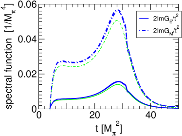
Figure 2: The isovector spectral functions in units of $m_{\pi}^{-4}$. Solid lines: $2\text{Im}G_{E}^{v}(t)/t^{2}$, dashed lines: $2\text{Im}G_{M}^{v}(t)/t^{2}$. The thin lines are from the work of Höhler and Pietarinen (1975), the thick lines include modern data for the pion form factor. The figure is from Belushkin et al. (2006).

The spatial distribution of charge and current can be obtained by the respective form factors in the Breit frame. The starting point is Eq. (34) for space-like $t=-Q^{2}\rightarrow-{\vec{q}\,^{2}}$, which is Fourier transformed to ${\vec{r}}$-space with the result

$$\rho(r)=\frac{1}{4\pi^{2}}\,\int_{t_{0}}^{\infty}dt\;{\rm{Im}}~{}G(t)\frac{e^{-\sqrt{t}\,r}}{r}\,.$$ (36)

The mean squared radius for a particular region of the spectral function at $t=\mu^{2}$, where $\mu$ is the mass of the intermediate state, is given by $<r^{2}>=6/\mu^{2}$. For instance, the onset of the spectral function corresponds to an rms radius of about 1.7 fm, the $\rho$ meson to about 0.6 fm, and so on. We conclude that the density at large distances is dominated by the lightest intermediate states. As a consequence, the tail of the density distribution at large radii should take a Yukawa form, $e^{-\mu r}/r$, with $\mu_{v}=2m_{\pi}$ and $\mu_{s}=3m_{\pi}$ for the isovector and isoscalar form factors, respectively. It is therefore natural to identify the “pion cloud” with the two-pion contribution to the spectral function, which remains after subtraction of the $\rho$ peak from the spectral function of Fig. 2. Whereas the isovector spectral function can be constructed from the available experimental information up to $t\approx 1~{}\text{GeV}^{2}$, the higher part of the spectrum has be modeled from information about resonances and continua. Because the isoscalar spectral function contains at least 3 pions in the intermediate state, it can not be obtained directly from experimental data. In the region below $t\approx 1~{}\text{GeV}^{2}$ it is dominated by the $\omega$ and $\Phi$ mesons, the three-pion continuum has been shown to couple only weakly, see Belushkin et al. (2007) and references to earlier work.

III Form factors

Figure 3: The world data for the 4 nucleon form factors according to Friedrich and Walcher (2003). The solid line is the phenomenological fit given by Eqs. (38) and (39). The other lines show the two dipole contributions and the bump/dip term of the fit separately. Note that the absolute value is plotted for negative quantities. See Friedrich and Walcher (2003) for a detailed listing of the data.

Ever since Hofstadter (1956, 1957) first determined the size of the nucleon, it has been taken for granted that the nucleon’s electromagnetic form factors follow the shape of a dipole form, with some minor deviations and, of course, modified for the vanishing charge of the neutron. This form was conveniently parameterized as

$$G(Q^{2})=\frac{1}{(1+Q^{2}/\Lambda_{D}^{2})^{2}}\,,$$ (37)

with $\Lambda_{D}\approx~{}0.84~{}$GeV a universal parameter. Because this parameter is close to the mass of the $\rho$ meson, it was assumed that the nucleon structure is dominated by a vector meson cloud which was described by the “vector dominance model”. This idea was of course in conflict with the quark model after its establishment in the 1970’s and many attempts were made to reconcile these conflicting models.

In order to set the scene, let us recall the following properties of proton, neutron, and heavier baryons:

• The complexity of these strongly interacting many-body system reflects itself in the finite size in space, the anomalous magnetic moment, and the continuum of excited states with strong resonance structures. These three aspects are of course closely related, and can be connected quantitatively in some cases by sum rules as detailed in section VI.

• Because of the approximate SU(3) symmetry of $u$, $d$, and $s$ quarks, the nucleon forms a doublet in isospin with strangeness $S=0$ in an octet of states. The other partners are: the $\Lambda^{0}$ and the triplet $\Sigma^{+},\Sigma^{0},\Sigma^{-}$ with $S=-1$, and the $\Xi^{0},\Xi^{-}$ with $S=-2$. The strange baryons decay weakly with a typical mean life of about $10^{-10}$ s. Because the $\Sigma^{0}$ can also decay into the $\Lambda^{0}$ by photoemission, its mean life is only about $10^{-19}$ s. The most important resonance of the nucleon, the $\Delta(1232)$ appears as an isospin quadruplet with strangeness $S=0$ in a decuplet of states. The partners of the $\Delta(1232)$ are: an isospin triplet $\Sigma^{+}(1385),\Sigma^{0}(1385),\Sigma^{-}(1385)$ with $S=-1$, a doublet $\Xi^{0}(1530),\Xi^{-}(1530)$ with $S=-2$, and the $\Omega^{-}(1672)$ with $S=-3$. The latter lives about $10^{-10}$ s, because it can only decay weakly. All the other particles in the decuplet decay by the strong interaction with a mean life of order $10^{-23}$ s.

• The size effect reflects itself in the form factors of elastic electron scattering. Because of the life time, only the proton and, with some caveat, the neutron can be studied as a target. With the dipole form of Eq. (37) and the definition of an rms radius according to Eq. (II.2), the result of Hofstadter (1956) was $r_{E}^{p}=0.81$ fm for the charge distribution of the proton. In the mean time several new experiments have led to the larger radius of $r_{E}^{p}\approx 0.88$ fm. The form factors of the strange baryons can in principle be measured by scattering an intense beam of these particles off the atomic electrons of some nuclear target. Such an experiment was performed by the SELEX Collaboration at the Fermi Lab Tevatron with a high-energetic $\Sigma^{-}$ beam Eschrich et al. (2001). The result is a first datum on a hyperon radius, $r_{E}^{\Sigma^{-}}=(0.78\pm 0.08\pm 0.05)$ fm, distinctly smaller than the accepted value for the proton.

• The “normal” magnetic moment of a particle i expected for a pointlike Fermion is given by $eQ_{i}/(2M_{i})$, with $M_{i}$ the mass and $e\,Q_{i}$ the charge of the particle. If the magnetic moments $\mu_{i}$ are given in units of the nuclear magneton $[\mu_{N}]=e/(2M_{p})$, the values for proton and neutron, $\mu_{p}=2.79~{}[\mu_{N}]$ and $\mu_{n}=-1.91~{}[\mu_{N}]$, signal a large isovector anomalous magnetic moment of the nucleon. From electron scattering we also know that the rms radius of the magnetization distribution is quite similar to the radius of the charge distribution. Because of their long mean life, the magnetic moments of 5 other octet baryons and, in addition, the one of the $\Omega^{-}(1672)$ in the decuplet are known from spin precession experiments. Without going in the details, also these particles have large anomalous moments. As an example, even the $\Omega^{-}$, a configuration of 3 $s$ quarks with the large mass of 1.672 GeV, has $\mu_{\Omega}=-2.02~{}[\mu_{N}]$ compared to a “normal” magnetic moment of $-0.56~{}[\mu_{N}]$. In order to get more information about the decuplet, several experiments were performed to measure the magnetic moment of the $\Delta^{++}$ as a subprocess of radiative pion-nucleon scattering Nefkens et al. (1978); Bosshard et al. (1991) and of the $\Delta^{+}$ as a subprocess of radiative pion photoproduction on the proton Kotulla (2003). The results for the magnetic moments are in qualitative agreement with quark model predictions but still with large model errors Pascalutsa and Vanderhaeghen (2007).

At the turn of the century new surprising results put the nucleon form factors into focus once more. These new results became possible through the new generation of cw electron accelerators with sources of high-intensity polarized beams combined with progress in target and recoil polarimetry. As summarized in section II.2 the measurement of asymmetries allows one to determine both form factors even if they are of very different size. This situation occurs in two cases: (I) Because of its vanishing total charge but large anomalous magnetic moment, the neutron’s electric form factor is very much smaller than the magnetic one, at least for small and moderate momentum transfer. (II) As shown by Eq. (15), the magnetic form factor $G_{M}(Q^{2})$ appears with a factor $\tau=Q^{2}/4M^{2}$, whereas $G_{E}(Q^{2})$ is suppressed by a factor $1/(1+\tau)$. As a consequence, $G_{E}(Q^{2})$ is less well determined by the Rosenbluth plot if $Q^{2}$ becomes large. Even though this was known, it was to the great surprise of everybody when asymmetry measurements showed a dramatic deviation from previous results based on the Rosenbluth separation and, at the same time, from the dipole shape of the proton form factors Jones et al. (2000); Gayou et al. (2002). Another open question concerns the behavior of the form factors at low 4-momentum transfer, such as oscillations at very small $Q^{2}$ and conflicting results for the rms radius of the proton. All these experimental findings have caused an intense theoretical investigation that has been summarized by several recent review papers Gao (2003); Hyde-Wright and de Jager (2004); Perdrisat et al. (2007); Arrington et al. (2007b). In the present work we concentrate on the low momentum transfers and, therefore, the phenomena for $Q^{2}\geq 1~{}\text{GeV}^{2}$ will only be discussed briefly.

III.1 Space-like electromagnetic form factors of the nucleon

The new results in the field of space-like form factors have been obtained at basically 3 facilities, the cw electron accelerators CEBAF at the Jefferson Lab Cardman (2006) and Mainz Microtron Jankowiak (2006), and the electron stretcher ring at MIT/Bates Milner (2006). All these facilities provide an intense beam of polarized electrons. The second essential for measuring the asymmetries was the development of polarized targets and polarimeters to determine the polarization of the recoiling particles. For details of the new accelerators, targets, and particle detectors as well as pertinent references, we refer the reader to a recent review of Hyde-Wright and de Jager (2004). In this context it is however important to realize that there exist no free neutron targets, but only targets with neutrons bound in a nucleus. Therefore, any analysis of the data requires theoretical models to correct for the binding effects, which include initial-state correlations, meson exchange and other two-body currents with intermediate resonance excitation of the nucleons, and final-state interactions while the struck nucleon leaves the target. In this situation, we infer that the deuteron provides the most trustworthy neutron target, because its theoretical description is far more advanced than in the case of heavier nuclei. Of course, measurements with heavier nuclei, in particular polarized ${}^{3}He$ targets, provide complementary information and are interesting for their own sake.

In Fig. 3 we display the nucleon form factors as functions of $Q$. We choose this somewhat unusual presentation in order to emphasize the small $Q^{2}$ region. The data base shown is from Friedrich and Walcher (2003), which meanwhile has been complemented by results from the following references: Crawford et al. (2007); Bermuth et al. (2003); Glazier et al. (2005); Plaster et al. (2006); Ziskin (2005); Anderson et al. (2007). The phenomenological fit shown by the solid line in Fig. 3 is composed of two dipoles and a bump/dip structure. The dipole form is given by

$$G_{s}(Q^{2})=\frac{a_{10}}{(1+Q^{2}/a_{11})^{2}}+\frac{a_{20}}{(1+Q^{2}/a_{21})^{2}}\,,$$ (38)

and the bump/dip structure, seen at $Q^{2}=Q_{b}^{2}\approx 0.2~{}\text{GeV}^{2}$ on top of the smooth dipoles, is parameterized as

$$G_{b}(Q^{2})=a_{b}\,Q^{2}\,\left(e^{\textstyle-\frac{1}{2}(\frac{Q-Q_{b}}{\sigma_{b}})^{2}}+e^{\textstyle-\frac{1}{2}(\frac{Q+Q_{b}}{\sigma_{b}})^{2}}\right)\,.$$ (39)

We note that this ansatz provides an even function of $Q$ as required by general arguments. A similar form has been introduced by Sick (1974) in r-space in order to obtain a non-singular function for his model-independent analysis of nuclear charge distributions.

Figure 4: The nucleon form factors $G_{E}^{p}$, $G_{M}^{p}/\mu_{p}$, and $G_{M}^{n}/\mu_{n}$ as function of $Q$, divided by the standard dipole form factor of Eq. (37). The full line represents the fit of Friedrich and Walcher (2003), the broken line shows the smooth contribution of the two dipoles.

Figure 5: The world data for the electric form factor of the neutron, $G_{E}^{n}$, as function of $Q^{2}$. Solid squares: $d(\vec{e},e^{\prime}\vec{n})p$ at MAMI, Ostrick (2006); Glazier et al. (2005), solid triangles: $d(\vec{e},e^{\prime}\vec{n})p$ at Jlab, Madey et al. (2003), solid diamond: $d(\vec{e},e^{\prime}\vec{n})p$ at BATES, Eden et al. (1994), solid circle: $\vec{d}(\vec{e},e^{\prime}n)p$ at NIKHEF, Passchier et al. (1999), open triangles: $\vec{d}(\vec{e},e^{\prime}n)p$ at Jlab, Warren et al. (2004), open diamonds: $\vec{d}(\vec{e},e^{\prime}n)p$ at BATES, Ziskin (2005), open squares: ${}^{3}\vec{He}(\vec{e},e^{\prime}n)pp$ at MAMI, Rohe (2006). The open circles are derived from the deuteron quadrupole form factor Schiavilla and Sick (2001). Solid line: new fit of the phenomenological model of Friedrich and Walcher (2003), dashed line: the result of dispersion relation Belushkin et al. (2007); Meißner (2007), dotted line: the original Galster fit of Eq. (40). The new fit includes all the shown data except for the preliminary of Ziskin (2005) and the values derived by Schiavilla and Sick (2001). The data in the figure were updated by J. Friedrich and the theory curves complemented by L. Tiator.

Figure 3 shows that the bump/dip structure is of the order 3% and only visible for $Q^{2}<1~{}\text{GeV}^{2}$. Therefore we have magnified the data and their structure by the linear plot of Fig. 4, which shows the form factors divided by the standard dipole form factor of Eq. (37). The electric form factor of the neutron is quite special because of its vanishing charge, which results in an overall small value of $G_{E}^{n}$. Therefore we have plotted this form factor in a different way in Fig. 5, which displays the published world data as measured with polarized electrons. We note, however, that the results of Schiavilla and Sick (2001) have been deduced from an analysis of the deuteron quadrupole form factor $F_{C2}$, which requires a careful investigation of the model dependence due to the nucleon-nucleon potential. The error bars of these data are therefore not statistical but indicate the (systematic) model error. The combined data shown in Fig. 5 clearly support the existence of the bump structure at $Q^{2}\approx 0.2~{}\text{GeV}^{2}$ as in the previous cases. The solid line in this figure is the result of a new fit with the phenomenological model given by Eqs. (38) and (39). The dashed line in this figure is the parameterization first given by Galster et al. (1971),

$$G_{E}^{n}(Q^{2})=\frac{a_{G}~{}\tau}{(1+b_{G}~{}\tau)}\cdot\frac{1}{(1+Q^{2}/\Lambda_{D}^{2})^{2}}\,,$$ (40)

with $a_{G}=-\mu_{n}$ and $b_{G}=5.6$. The result from dispersion theory is displayed by the dotted line. Neither dispersion theory nor the Galster fit reproduce the data at low $Q^{2}$.

The Fourier transform of $G_{E}^{n}$ is of particular interest, because the overall charge of the neutron must vanish. A finite charge distribution is therefore a definite sign of correlations among the charged constituents, for example, between the $u$ quark and the two $d$ quarks of the constituent quark model. The charge distribution $\rho_{E}^{n}$ is displayed in Fig. 6 for the 3 fits to the neutron factor shown in the previous figure.

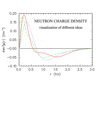
Figure 6: The charge density distribution for the neutron, $4\pi r^{2}\rho_{E}^{n}$, as function of $r$. The notation for the lines corresponds to that of the form factors shown in Fig. 5. Figure by courtesy of J. Friedrich and L. Tiator.

We recall the arguments of subsection II.2 that the Fourier transform can only be obtained in the Breit or “brick wall” frame, which however is a different Lorentz frame for different values of $Q^{2}$. The visualization of the Fourier transforms as charge and magnetization distributions in r-space is therefore only approximately correct if the momentum transfer is small compared to $|Q^{2}|=4M^{2}$, which defines the threshold of nucleon pair production at time-like momentum transfer. With this caveat in mind, we may interpret the charge distribution of Fig. 6 by the dissociation of the neutron in a proton and a pion, i.e., as a negative “pion cloud” around a positive core. As we see from the figure, the pion cloud found by Friedrich and Walcher (2003) extends to large radii. It is important to realize that this result does not depend on a model assumption but is borne out by a statistically satisfactory reproduction of the data. We also note that the signal of the pion cloud is empirically present in all 4 form factors.

In a recent paper, Miller (2007) has found a negative density in the center of the neutron from an analysis of generalized parton distributions as function of the impact parameter $b$. The charge distribution $\rho_{1}^{n}(b)$ is then defined by the 2-dimensional Fourier transform of the Dirac form factor $F_{1}^{n}(Q^{2})$. We note that this does not contradict the results shown in Fig. 6. In fact our results for the 3-dimensional Fourier transform of $F_{1}^{n}(Q^{2})$ agree very much with the findings of Miller (2007): a negative density in the center, positive values for $0.4$ fm$<r<1.2$ fm, and a negative tail for the larger distances.

III.2 Time-like electromagnetic form factors of the nucleon

Figure 7: The world data for the time-like form factor of the proton as function of the beam energy $E_{\text{beam}}$, extracted with the assumption $|G_{E}|=|G_{M}|$. Open symbols: data from $e^{+}e^{-}\rightarrow p\bar{p}$ Antonelli et al. (1996); Delcourt et al. (1979); Bisello et al. (1983, 1990); Castellano et al. (1973); Antonelli et al. (1998); Ablikim et al. (2005); Pedlar et al. (2005); Aubert et al. (2006), solid symbols: data from $\bar{p}p\rightarrow e^{-}e^{+}$ Bassompierre et al. (1977); Bardin et al. (1994); Armstrong et al. (1993); Ambrogiani et al. (1999); Andreotti et al. (2003). The figure is from Rossi et al. (2006).

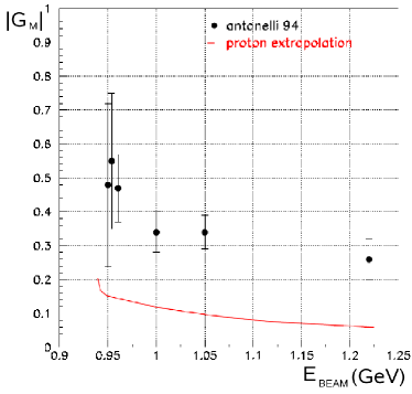
Figure 8: The world data for the time-like form factor of the neutron as function of the beam energy $E_{\text{beam}}$, extracted with the assumption $|G_{E}|=|G_{M}|$. The data are obtained by the FENICE collaboration from the reaction $e^{+}e^{-}\rightarrow n\bar{n}$. The solid line is a perturbative QCD extrapolation using the proton data Antonelli et al. (1998, 1994). The figure is from Rossi et al. (2006).

Let us next discuss the form factors for time-like momentum transfer, i.e., positive values of the Mandelstam variable $t=q^{2}=-Q^{2}>0$, see subsection II.1 for definitions. By inspection we find that the previously defined dipole form factors have poles $t=\Lambda_{D}^{2}\approx M_{V}^{2}$, that is, the phenomenological fits “predict” the existence of vector mesons in the time-like region. The form factors in the space-like and time-like regions are connected by analyticity and unitarity, and therefore also the knowledge of the time-like form factors is mandatory for a complete understanding of the nucleon Baldini et al. (1999); Geshkenbein et al. (1974); Hammer (2006); Mergell et al. (1996); Belushkin et al. (2007). The time-like photons are obtained in collider experiments by the reaction $e^{+}e^{-}\rightarrow N\,{\bar{N}}$ for $t=(2E_{\text{beam}})^{2}>4M^{2}$. Whereas the space-like form factors are real, the time-like form factors are complex functions because of the strong interaction between the produced hadrons. However, the unpolarized cross section in the time-like region only depends on the absolute values of the two form factors, $|G_{E}(t)|$ and $|G_{M}(t)|$. In order to get information on the relative phase between the form factors, polarization experiments are required. Unfortunately, the present data basis does not even allow for a Rosenbluth separation. Therefore the data are analyzed with the assumption $|G_{E}(t)|=|G_{M}(t)|$, which follows from Eq. (13) at threshold, $t=4M^{2}$, but is of course not expected to hold for higher beam energies.

Figure 7 displays a compilation of the proton data known so far. These data cover the range of $4M^{2}<t<6.8~{}\text{GeV}^{2}$. The figure shows an overall falloff with the beam energy for $G_{M}^{p}$, somewhat faster than $1/t^{2}$, and some structure near $E_{\text{beam}}=1.05$ GeV or $t=4.4~{}\text{GeV}^{2}$, which may indicate a resonance in that region. We note that the decrease of the form factor is in qualitative agreement with perturbative QCD, which requires a falloff like $|t|^{-2}$ for both space-like and time-like photons. However, a comparison shows that the space-like form factor at $t=-Q^{2}=-16~{}\text{GeV}^{2}$ is already about a factor 3 smaller than the time-like form factor at $t=+16~{}\text{GeV}^{2}$, that is, asymptotia is still far away. A look at Fig. 8 tells us that our knowledge about the neutron’s time-like form factors is still far from satisfactory. We hope that the currently planned experiments will improve on the precision of the time-like form factors and, in particular, also determine their relative phases, which is absolutely necessary in order to get the full information on the structure of the nucleon Rossi et al. (2006).

III.3 Theoretical considerations

The electromagnetic form factors encode information on the wave functions of the charged constituents in a bound system. However, in the case of the hadrons we face severe obstacles to get a real grip on the elementary quarks. As has been mentioned in section I, only two ab-initio approaches exist to describe QCD in the confinement phase, chiral perturbation theory and lattice gauge theory. Chiral perturbation theory is restricted to small values of the momenta. Moreover, if extended to higher order in the perturbation series, ChPT loses predictive power, because the number of unknown low energy constants increases. Lattice gauge theory, on the other hand, is still hampered by the use of large quark masses. This has the consequence that the pionic effects appearing at low momentum transfer are underestimated. Beyond these two approaches, which are in principle exact realizations of QCD, a plethora of “QCD inspired” models with quarks and pions has been developed. The problems are twofold:

• Starting directly from QCD, one would have to use the small $u$ and $d$ quark masses of order 10 MeV. The many-body system is therefore highly relativistic from the very beginning. However, a typical constituent quark model (CQM) has quarks with masses of several hundred MeV. It is therefore obvious that these entities are many-body systems of quarks and gluons by themselves. In any case, the constituent quarks wave functions have to “boosted” if hit by the virtual photon. However, there exists no unique scheme to boost a strongly interacting relativistic many-body system.

• In view of the small current mass of the quarks, the interaction as mediated by gluon exchange inevitably produces a considerable amount of quark-antiquark admixture. These effects have to be modeled by properties of the constituent quarks, such as mass and form factor, see De Sanctis et al. (2005a), or by explicitly introducing a meson cloud of the “bare” constituent quarks Faessler et al. (2006).

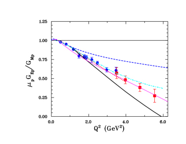
Figure 9: The ratio of the electric and magnetic form factors of the proton, $\mu_{p}\,G_{E}^{p}/G_{M}^{p}$, compared to relativistic calculations in the framework of the CQM. Dotted line: light-cone front CQM Chung and Coester (1991), thick solid line: light-cone front CQM Frank et al. (1996), dashed-dotted line: light-cone front CQM with point-like constituent quarks  Cardarelli et al. (1995); Cardarelli and Simula (2000), dashed line: Goldstone boson exchange between point-like constituent quarks Boffi et al. (2002), thin solid line: covariant spectator CQM Gross and Agbakpe (2006). The data have been taken at Jefferson Lab by Punjabi et al. (2005) (circles) and Gayou et al. (2002) (squares). The figure is from Perdrisat et al. (2007).

Since this article is dedicated to the low-$Q^{2}$ domain, it suffices to consider some models useful in this region. A more detailed discussion of the wide range of models is given by Perdrisat et al. (2007). The traditional model of the nucleon is the CQM with quark masses $m_{q}\approx M/3$. Except for the smallest momentum transfers, the quark wave functions have to be relativized, which is usually done by relativistic boosts of the single-quark wave functions. Figure 9 shows the result of several calculations for the ratio $G_{E}^{p}/G_{M}^{p}$ compared to the recent data from the Jefferson Lab obtained with a double-polarization experiment. The rapid falloff of this ratio was a real surprise, because previous experiments without polarization did not find big deviations from the dipole fit for both form factors. The solution of problem was explained by two-photon effects, which are usually small but turn out to become large in special cases, see Carlson and Vanderhaeghen (2007) and Arrington et al. (2007a) for recent reviews. Even though the figure shows only a small selection of models, quite different results are obtained by similar models, depending on the properties of the constituent quarks, their interaction, and the boosting mechanism. We are also not aware of many predictions for the rapid drop of the ratio, before the JLab double-polarization data were obtained. In any case, the shown models describe the data qualitatively well, and they support the expected zero crossing of the electric form factor at $Q^{2}\approx 7~{}\text{GeV}^{2}$. The zero crossing is also predicted from a Poincaré covariant Faddeev calculation describing the nucleon as a correlated quark-diquark system, generated with an interaction fitted to the structure of mesons Alkofer et al. (2005); Höll et al. (2005). On the other hand, the models without explicit Goldstone bosons, in particular pions, can not describe the region of $Q^{2}\lessapprox 0.5~{}\text{GeV}^{2}$, in which the pionic degrees of freedom play a decisive role.

The inclusion of a pion cloud into quark models of the nucleon started with the “little bag model” Brown and Rho (1979) and was first applied to the nucleon form factors in the form of the “cloudy bag model” Thomas (1984); Lu et al. (1998); Miller and Frank (2002); Miller (2002). More recently, Pasquini and Boffi (2007) studied a system of valence quarks surrounded by a meson cloud with light-cone wave functions. They found distinct features of such a cloud below $Q^{2}=0.5~{}{\text{GeV}}^{2}$, however without a pronounced bump-dip structure. Another model incorporating quarks and Goldstone bosons is the “chiral quark soliton model” Diakonov and Petrov (1986); Diakonov et al. (1988). The nucleon form factors were calculated within this framework by Christov et al. (1995). The linear decrease of the ratio $G_{E}^{p}/G_{M}^{p}$ with $Q^{2}$ was shown to follow from this model quite naturally Holzwarth (1996, 2002, 2005). However, in all of these models the bump/dip structure of the form factors is not in focus. On the other hand, Faessler et al. (2006) showed that this structure can be reproduced within a chiral quark model by a cloud of pseudoscalar mesons. One should also keep in mind that usually the authors do not give a complete description of the data. For example, a cross section ratio may be obtained in agreement with the data, whereas the model fails to describe the individual cross sections. On the contrary, the parameterization of Friedrich and Walcher (2003) covers the full $Q^{2}$ domain up to 7 GeV², and therefore the charge distribution derived from this work is directly based on the experimental data. As is obvious from Fig. 6, the neutron charge distribution $\rho_{E}^{n}(r)$, as defined by the Fourier transform of the electric Sachs form factor $G_{E}^{n}(Q^{2})$, is positive in the interior region and negative for radii larger than about 0.7 fm. However, it certainly takes a model to quantify the separation into components, say a core and a “pion cloud”. As an example, there is no unique way to break the spectral function of Fig. 2 into parts belonging to the two-pion continuum and heavier intermediate states like the $\rho$ meson. On the other side, it is also evident that the tail of the density at large radii is determined by the lightest hadron, the pion.

Since the size of the bump/dip signal found by Friedrich and Walcher (2003) (FW) is in conflict with calculations using dispersion relations Belushkin et al. (2007); Meißner (2007) (BHM), it is worthwhile to discuss the differences more closely.

• The fit of FW describes the data in the space-like region with a very good $\chi^{2}/\text{dof}\approx 0.9$ for about 160 degrees of freedom (dof), because the fitting function is designed for the space-like data. The dispersion relations try to reproduce both the space-like and the time-like form factors by use of all the available spectral data for the involved hadrons, and therefore the fits are much more constrained. As a result, the fits of BHM have the much larger $\chi^{2}/\text{dof}\approx 1.8$ with $\text{dof}\approx 200$. Such large values of $\chi^{2}$ have to be taken with great caution since they are somewhat outside the range of the validity of statistics. In particular, the statistical probability $P(\chi^{2}/\text{dof}>1.8,\,\text{dof}\approx 200)$ is smaller than $10^{-10}$. This leaves the usual suspects: the problem is in the data Belushkin et al. (2007); Meißner (2007), the dispersion relation have still an incomplete input, or both data and theory have problems. In any case, the 1-$\sigma$ bands of Belushkin et al. (2007) and Meißner (2007) derived by increasing the absolute $\chi^{2}$ by 1 are not meaningful if the $\chi^{2}/\text{dof}$ is as much off as $1.8$.

• In order to obtain the bump/dip structure at $Q^{2}\approx 0.2~{}\text{GeV}^{2}$, BHM would have to include two more “effective” poles: an additional isoscalar pole near the (isoscalar) $\omega$ meson, but with the opposite sign and twice the strength of the $\omega$, and a weaker isovector structure close to the mass of 3 pions, which is the threshold of the isoscalar channel. With these modifications, also BHM could obtain a $\chi^{2}/\text{dof}\approx 0.9$. There is however no evidence for such structures in ${e^{+}}-{e^{-}}$ collisions nor are such objects known to interact with the nucleon, and therefore BHM discard these fits.

• The electric rms radius of the proton, $r_{E}^{p}$, is another piece of evidence showing some peculiarity around $0.2~{}\text{GeV}^{2}$. From a fit to all the available low $Q^{2}$ data, Sick (2003) finds the radius $r_{E}^{p}=(0.95\pm 0.018)$ fm . On the other hand, FW obtain $r_{E}^{p}=0.794$ fm without and $r_{E}^{p}=0.858$ fm with the bump/dip structure. According to Rosenfelder (2000), Coulomb and recoil corrections have to be added to these results, which leads to $r_{E}^{p}=0.876\pm 0.015$ fm in accord with results from Lamb shift measurements Udem et al. (1997). (For an overview of the results from atomic physics and their interpretation, we refer to the work of Karshenboim (1998) and Carlson and Vanderhaeghen (2007).) However, as in all previous work based on dispersion relations, the electric rms radius of the proton also turns out to be small in the work of BHM, $r_{E}^{p}=0.844$ fm or even smaller.

• The dip structure reported by FW for the proton corresponds to a bump structure obtained for the neutron at a similar value of $Q^{2}$. This change of sign makes sense, because the pion cloud couples to the isovector photon. As mentioned before, Kopecky et al. (1997) obtained a mean square radius $\langle r^{2}\rangle_{E}^{n}=-(0.115\pm 0.004)~{}\text{fm}^{2}$ from low-energy neutron scattering off ²⁰⁸Pb, however this extraction is certainly model dependent. BHM get $\langle r^{2}\rangle_{E}^{n}=-0.118~{}\text{fm}^{2}$, in agreement with Kopecky et al. (1997). FW take $\langle r^{2}\rangle_{E}^{n}=-0.115$ fm as a fixed parameter or obtain $\langle r^{2}\rangle_{E}^{n}=-0.147$ fm in the new fit of the analytical form of the phenomenological model.

• It follows from dispersion relations that the tail of the charge distributions at large radii has a Yukawa shape with the mass of the lightest intermediate state, that is the 2 pion masses for the isovector and 3 pion masses for the isoscalar densities. Hence it would take a considerable cancellation of positive and negative structures in the lower part of the spectral function if one wants to shift the pion cloud to rms radii above 1.7 fm. This is in conflict with the bump/dip structure of Eq. (39), which results in a considerable amount of charge in the “pion cloud” above 1.7 fm, as seen in Fig. 6.

• The fit of FW is restricted to the space-like form factors. This approach can not be extended to the time-like region, and another purely empirical fit would make little sense in view of the restricted data basis in the this region. The dispersion relations, on the other hand, are built just to make the connection between the two regions, and the results of BHM give a good overall description in both domains. However, they miss a structure at $E_{\text{beam}}\approx 1.05\,$GeV or $t\approx 4.4~{}\text{GeV}^{2}$.

In concluding these arguments, we mention that dispersion theory and FW agree on the dip seen for the magnetic form factors of both proton and neutron at $Q^{2}\approx 0.2~{}\text{GeV}^{2}$. There is also qualitative agreement that the charge and the magnetization in the surface region of the nucleon, $r\gtrapprox 1$ fm, are dominated by the pion cloud, which reaches much beyond the rms radius of the proton. It remains a challenge for both experiment and theory to answer the raised questions concerning the distributions of charge and magnetization inside an nucleon, which we consider a key aspect of the nucleon structure.

III.4 Weak form factors of the nucleon

III.4.1 Axial form factor of the nucleon

The axial current of the nucleon can be studied by anti-neutrino and neutrino scattering, pion electroproduction, and radiative muon capture, see Bernard et al. (2002a); Gorringe and Fearing (2004) for recent reviews. The (isovector) axial current between nucleon states takes the form

$$A_{\mu}=\bar{u}_{p_{2}}\left(\gamma_{\mu}\,G_{A}(Q^{2})+i\frac{(p_{2}-p_{1})_{\mu}}{2M}\,G_{P}(Q^{2})\right)\gamma_{5}\,u_{p_{1}}\,.$$ (41)

As for the vector current, Eq. (11), there appear two form factors, the axial form factor $G_{A}$ and the induced pseudoscalar form factor $G_{P}$. A linear combination of the form factors $G_{A}$ and $G_{P}$ is related to the pion-nucleon form factor $G_{\pi\,N}$ by the PCAC relation. The experimental information about the induced pseudoscalar form factor is limited. The data are mostly obtained from muon capture by the proton, $\mu^{-}+p\rightarrow n+\nu_{\mu}$. This determines the value of $G_{P}$ at $Q^{2}=0.88\,m_{\mu}^{2}\approx 0.01$ GeV², which is usually described by the induced pseudoscalar coupling constant, $g_{P}=\frac{m_{\mu}}{2M}G_{P}(Q^{2}=0.88\,m_{\mu}^{2})$. A recent experiment at PSI yielded the value $g_{P}=7.3\pm 1.1$ Andreev et al. (2007), in agreement with the result from heavy baryon ChPT Bernard et al. (2002a), $g_{P}=8.26\pm 0.16$, and manifestly Lorentz-invariant ChPT Schindler et al. (2007), $g_{P}=8.29\pm 0.7$, with an estimated error stemming mostly from the truncation of the chiral expansion. The axial form factor $G_{A}$ is usually parameterized in the dipole form of Eq. (37), with a parameter $\Lambda_{A}$ called the “axial mass”,

$$G_{A}(Q^{2})=\frac{g_{A}}{(1+Q^{2}/\Lambda_{A}^{2})^{2}}\,$$ (42)

with $g_{A}=1.2695(29)$ Yao et al. (2006). A recent (corrected) global average of the axial mass as determined by neutrino scattering has been given by Budd et al. (2003),

$$\Lambda_{A}^{\nu}=(1.001\pm 0.020)~{}\text{GeV}\,.$$ (43)

However, quite a different value, $\Lambda_{A}^{\nu}=(1.20\pm 0.12)~{}\text{GeV}$ has been derived by the K2K Collaboration from quasi-elastic $\nu_{\mu}n\rightarrow\mu^{-}p$ in oxygen nuclei Gran et al. (2006). The axial form factor has also been studied by pion electroproduction Baumann (2005). The Rosenbluth separation of these data is shown in Fig. 10. The results are in agreement with an earlier experiment by Liesenfeld et al. (1999), but are complemented by a data point at the very low momentum transfer of $Q^{2}=0.058~{}\text{GeV}^{2}$. An exact Rosenbluth separation is prerequisite, because the transverse cross section $\sigma_{T}$ is sensitive to $G_{A}$ and the longitudinal cross section to the pion form factor $F_{\pi}$, which is discussed in subsection III.5. These electroproduction data have been analyzed with MAID2007 as follows: (I) The cross sections $\sigma_{T}$ and $\sigma_{L}$ of MAID were normalized to the data by factors 0.825 and 0.809, respectively, and (II) the axial dipole mass $\Lambda_{A}$ and the corresponding “mass” for the monopole form of the pion form factor were fitted. The result is $\Lambda^{\pi}_{A}=(1.028\pm 0.025)$ GeV. However, this value has to be corrected for the “axial mass discrepancy”, $\Lambda^{\pi}_{A}-\Lambda^{\nu}_{A}\approx 0.055$ MeV, which is due to loop corrections Bernard et al. (1992). With this correction, the electroproduction data of Baumann (2005) yield

$$\Lambda_{A}^{\text{corr}}=(0.973\pm 0.025)~{}\text{GeV}\,,$$ (44)

which agrees with the corrected value from neutrino scattering given by Eq. (43), but disagrees with both the previous result of Liesenfeld et al. (1999) and the measurement of Gran et al. (2006). In view of the relatively large normalization factor applied to the electro-production data, it would be helpful to check the normalization at $Q^{2}=0$ by pion photoproduction.

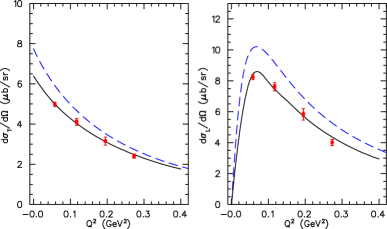
Figure 10: The transverse and longitudinal cross sections for charged pion production as function of $Q^{2}$. The data are from Baumann (2005). Dashed lines: cross sections predicted by MAID2007 Drechsel et al. (2007), solid lines: fit to the data with MAID2007 (See text for details.) Figure by courtesy of L. Tiator.

III.4.2 Strangeness content of the nucleon

As outlined in subsection II.3, the parity violating component of electron scattering provides access to the weak form factors $\tilde{G}_{E}$ and $\tilde{G}_{M}$. These form factors are related to the strangeness content of the nucleon by the universality of the electroweak interaction with the quarks. For a detailed derivation of the strange form factors and their experimental determination see, e.g., the review of Beck and McKeown (2001). Because the strangeness in the nucleon appears only through the presence of the heavy $s\bar{s}$ pairs, these observables are of great importance for our understanding of the nucleon in terms of large vs. small scales. The strangeness content is related to the $\sigma$ term, which has been derived from pion-nucleon scattering at the (unphysical) Cheng-Dashen point, $s=u=M^{2},\,t=2m_{\pi}^{2}$ Thomas and Weise (2001); Sainio (2002). This term is a direct measure of the chiral symmetry breaking in QCD, the chiral properties of the strong interactions, and the impact of sea quarks on the nucleon’s properties. Its relation to the strangeness contribution is given by

$$\sigma=\frac{\langle N|\bar{m}(\bar{u}u+\bar{d}d-2\bar{s}s)|N\rangle}{1-y}\,,$$ (45)

where $\bar{m}=(m_{u}+m_{d})/2$ is the average of the $u$ and $d$ quark masses, and $y$ is a measure for the scalar strange quark content of the nucleon,

$$y=\frac{2\langle N|\bar{s}s|N\rangle}{\langle N|\bar{u}u+\bar{d}d|N\rangle}\,.$$ (46)

From a recent detailed analysis, Pavan et al. (2002) found the value $y\approx 0.46$, indeed a surprisingly large strangeness content in the nucleon, whereas a much smaller value was obtained in earlier work Sainio (2002). These inconsistencies were a very strong motive to study the strangeness content with the electromagnetic probe. At large momentum transfer, $1~{}\text{GeV}^{2}\leqslant Q^{2}\leqslant 100~{}\text{GeV}^{2}$, the strangeness contribution has been derived from unpolarized deep-inelastic lepton scattering at the Fermi Lab Tevatron Bazarko et al. (1995). The momentum fraction of the sea quarks carried by the strange quarks extracted is

$$\kappa=\frac{\langle x(s(x)+\bar{s}(x))\rangle}{\langle x(\bar{u}(x)+\bar{d}(x))\rangle}\approx 0.5\,,$$ (47)

or about 3% of the total nucleon momentum. If this contribution is extrapolated to large spatial scales by the quark evolution, a rather small value is obtained.

On the theoretical side a plethora of nucleon models have usually predicted strangeness form factors of considerable size, see for example the review of Beck and Holstein (2001). These considerations have initiated an intense experimental program at several laboratories. These activities started at the Bates/MIT laboratory with the SAMPLE experiment, which first proved that it is feasible to measure the small asymmetries of order $10^{-6}$ in parity-violating electron scattering Spayde et al. (2004); Kowalski (2006). This experiment was based on a particular technique using Cherenkov detectors developed previously for a parity-violation experiment at the Mainz linac Heil et al. (1989) and an improvement of the SLAC polarized electron source Souder et al. (1990). At the Mainz Microtron MAMI, the A4 collaboration built a Cherenkov detector consisting of 1022 PbF₂ crystals, which in conjunction with electronics allowing for on-line identification of electromagnetic clusters, made it possible to count single events Maas (2006). Furthermore, two experiments were performed at the Jefferson Lab. The first of these experiments (HAPPEX) used the two-spectrometer set-up of Hall A taking advantage of a pair of septum magnets for measurements at very small scattering angles and low momentum transfers. This project was passing through different phases of improvement. HAPPEX-I measured on a hydrogen target Aniol et al. (2004) at $Q^{2}=0.48~{}\text{GeV}^{2}$ only. In this geometry the combination $G^{s}_{E}+0.392~{}G^{s}_{M}=0.014\pm 0.020\pm 0.010$ was determined. In the next step HAPPEX-II measured on both hydrogen Aniol et al. (2006a) and helium targets Aniol et al. (2006b). The nucleus ⁴He is quite special as a target, because only the electric form factor can contribute due to its zero total spin. The results of HAPPEX are compared to those of other collaborations in Fig. 11. Each measurement gives an error band in the plot of $G^{s}_{E}$ versus $G^{s}_{M}$. The common error ellipse indicates values for $G_{E}(0.1~{}$GeV${}^{2})$ and $G_{M}(0.1~{}$GeV${}^{2})$ that are consistent with zero but at variance with most theoretical predictions, however, not incompatible with the experiments obtained with the other methods mentioned above.

Figure 11: The strangeness form factors $G^{s}_{E}$ and $G^{s}_{M}$ at $Q^{2}=0.1~{}$GeV² as obtained by the SAMPLE, A4, HAPPEX, and G0 experiments. The bands represent the one-sigma (statistical plus systematical) error of the individual experiments, the ellipse is the combined two-sigma area for all measurements. The figure is from Kowalski (2006).

Recently the second phase of HAPPEX-II was completed, with the result of a much improved precision Acha et al. (2007). These results are compared with several theoretical predictions in Fig. 12. As is obvious from the figure, the strangeness form factors are centered about zero, whereas most of the models predict large values. The only theoretical results compatible with these experiments are from lattice gauge calculations with chiral extrapolation to the physical pion mass Lewis et al. (2003); Leinweber et al. (2005, 2006). The second JLab experiment was performed by the G0 collaboration. This collaboration has built an eight-sector superconducting toroidal magnetic spectrometer Armstrong et al. (2005). Figure 13 displays the $Q^{2}$ dependence of the world data including the G0 results. From this figure we get the impression of a small but finite value for that particular combination of the two strangeness form factors.

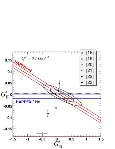
Figure 12: The one-sigma band of HAPPEX-II together with the one- and two-sigma ellipses derived by Acha et al. (2007). The theoretical predictions with their estimate errors are identified by the numbers given in the figure: [18] Park and Weigel (1992), [19] Hammer et al. (1996), [20] Hammer and Ramsey-Musolf (1999), [21] Silva et al. (2002), [22] Lewis et al. (2003), [23] Leinweber et al. (2005, 2006).

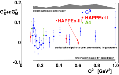
Figure 13: The form factor combination $G^{s}_{E}(Q^{2})+\eta G^{s}_{M}(Q^{2})$ as obtained by kinematical extrapolation from A4, HAPPEX II, and G0 experiments. The point “HAPPEX III” indicates the error bar for a planned measurement. The figure is from Kowalski (2006).

III.5 Form factor of mesons

Because mesons are unstable particles, their form factors can not be measured directly by lepton scattering but have to be obtained by more indirect methods. In the following we concentrate on the form factor of the charged pion, however similar methods can also be used to measure the form factors of heavier mesons or rare decays Guidal et al. (1997); Vanderhaeghen et al. (1998). At present, only the data for the pion are precise enough to allow for a reliable extraction of the form factors over a large region of momentum transfer. There exist two experimental methods to overcome the missing target problem. The first method is the scattering of relativistic mesons with dilated lifetime on atomic electrons, which are then identified by measuring the recoil of the struck electron. This method is limited to relatively small momentum transfer, $Q^{2}<0.5~{}\text{GeV}^{2}$. As a consequence, this method is essentially sensitive to the rms radius of the free pion, $r_{\pi}=\sqrt{\langle r^{2}\rangle_{\pi}}$, which is related to the mass parameter $\Lambda_{\pi}^{2}$ in the usual monopole form as follows:

$$F_{\pi}(Q^{2})=\frac{1}{1+Q^{2}/\Lambda_{\pi}^{2}}=1-\frac{1}{6}\,Q^{2}\,\langle r^{2}\rangle_{\pi}+{\mathcal{O}}~{}(Q^{4})\,.$$ (48)

From an experiment at the CERN SPS, Amendolia et al. (1984, 1986b) derived the rms charge radius of the pion, $r_{\pi}=(0.663\pm 0.006)~{}$fm. At the same time also the kaon form factor was measured Amendolia et al. (1986a). The rms charge radius of the charged kaon was found to be $r_{K}=(0.58\pm 0.05)~{}$fm, somewhat smaller than the pion radius, which is to be expected because of the heavier strange quark in the kaon. Because of the small momentum transfer involved, these results depend only little on the monopole form of the ansatz.

The second possibility to study the pion form factor is given by electron scattering on the pion cloud of the nucleon, which is part of the reaction $p(e,e^{\prime}\pi^{+})n$. The obvious problem is that the initially bound pion is off its mass-shell and that many other diagrams contribute as well. The idea is therefore to study this process in kinematic regions for which the t-channel pion exchange is dominant. In principle one should extrapolate the cross section to the pion pole, which however lies at the unphysical 4-momentum transfer $t=m_{\pi}^{2}$. At very high momentum transfer, $Q^{2}\gg 1~{}$GeV², this extrapolation can be performed within the Regge model Vanderhaeghen et al. (1998). Following this approach, Horn et al. (2006) have recently determined $F_{\pi}$ by a Rosenbluth separation of the longitudinal and transverse cross sections at the Jefferson Lab. In this way they extracted two precise values of the pion form factor at $Q^{2}=1.60~{}\text{GeV}^{2}$ and $2.45~{}\text{GeV}^{2}$, which are shown together with previous data and several model calculations in Fig. 14. Beside the model dependence on the Regge analysis, another problem arises because the data at the higher momentum transfer do not follow the monopole form, i.e., the value of $\Lambda_{\pi}^{2}$ differs by as much as 7% from $\Lambda_{\pi}^{2}$ = 0.53 GeV² as obtained by Amendolia et al. (1986b). This leads to an inconsistency of about 1 standard deviation. At small values of $Q^{2}$ one can also try to derive the rms radius from pion electroproduction as pointed out in subsection III.4.1. A previous result yielded $\Lambda^{2}_{\pi}=0.425~{}\text{GeV}^{2}$, equivalent to an rms radius $r_{\pi}=(0.74\pm 0.03)~{}$fm Liesenfeld et al. (1999). This result is clearly at variance with the value of Amendolia et al. (1986b). A reason for this discrepancy was given by Bernard et al. (2000); Bernard et al. (2002a) in terms of the loop corrections for the longitudinal s-wave multipole $L_{0+}^{(-)}$, which dominates the cross section $\sigma_{L}$ at small $Q^{2}$. In fact, these loop corrections increase the downward slope of $L_{0+}^{(-)}$ substantially, such that

$$\langle r^{2}\rangle_{\pi}[p(e,e^{\prime}\,\pi^{+})n]=\langle r^{2}\rangle_{\pi}+0.266~{}{\text{fm}}^{2}\,.$$ (49)

With the pion radius according to Amendolia et al. (1984, 1986b), $\langle r^{2}\rangle_{\pi}=0.440$ fm², the electroproduction experiment should therefore measure $\langle r^{2}\rangle_{\pi}[p(e,e^{\prime}\,\pi^{+})n]=0.706~{}\text{fm}^{2}$ or an “effective” rms radius of 0.84 fm, which is surprisingly close to the nucleon radius. The fit with MAID07 to the data of Baumann (2005) yields $\Lambda^{2}_{\pi}=(0.386\pm 0.042)~{}\text{GeV}^{2}$, which is smaller than the result of Liesenfeld et al. (1999). If we include the loop correction, we obtain $r_{\pi}=(0.78\pm 0.04)$ fm, which is quite close to the prediction of ChPT. Of course, there are weak points in our reasoning. In the first place, there is the already discussed overall reduction of the MAID model to fit the data. Second, the s-wave yields only about half of the measured cross section, and much smaller loop corrections are expected for the higher partial waves. Nevertheless we may conclude that the virtual constituent pion looks quite different from the free pion and appears, in this particular experiment, nearly as large as the nucleon.

Because the neutral pion is its own antiparticle, its form factor vanishes identically. However, the reaction $\gamma*(Q^{2})+\gamma\rightarrow\pi^{0}$ can be studied as function of $Q^{2}$. This provides information on the transition form factor $F_{\gamma*\gamma\pi^{0}}$ of the Wess-Zumino-Witten anomaly defined by Eq. (4) of section I. As shown in section IV this anomaly is quite important in Compton scattering and in particular for the spin polarizability of the nucleon. The transition form factor $F_{\gamma*\gamma\pi^{0}}$ was measured at the $e^{+}\,e^{-}$ collider at Cornell by the CLEO collaboration Gronberg et al. (1998) and at the PETRA storage ring by the CELLO collaboration Behrend et al. (1991). Analyzed with a monopole form factor as given by Eq. (48), these experiments yielded the parameter $\Lambda_{\gamma*\gamma\pi^{0}}=(776\pm 10\pm 12\pm 16)$ MeV, and similarly for the corresponding transition form factor of the $\eta$ meson $\Lambda_{\gamma*\gamma\eta}=(774\pm 11\pm 16\pm 22)$ MeV. Both results confirm the prediction of the vector dominance model assuming that the virtual photon coexists with the neutral $\rho$ meson, which decays in a pion or an $\eta$ and a real photon. The $Q^{2}$ dependence of the transition is then simply given by the propagator of the $\rho$, that is, $\Lambda\approx m_{\rho}=775.5$ MeV for both reactions. With the same arguments as for the ordinary form factors, we can turn this value in a transition radius $r_{\rm WZW}=0.62$ fm.

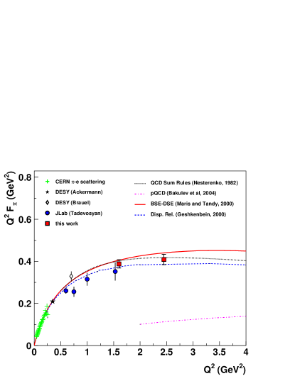
Figure 14: The pion form factor $F_{\pi}$ multiplied with $Q^{2}$. Crosses: Amendolia et al. (1984, 1986b) ($\pi-e$ scattering at CERN), asterisks: Ackermann et al. (1978) (DESY), diamonds: Brauel et al. (1977, 1979) (DESY), circles: Tadevosyan et al. (2007) (Jefferson Lab), and squares: Horn et al. (2006) (Jefferson Lab). The experimental results are compared to four model calculations as indicated by the lines. Figure from Horn et al. (2006).

IV Polarizabilities

The polarizability measures the response of a system to a quasi-static electromagnetic field. In particular the energy of a homogeneous and isotropic system is described by the electric ($\alpha_{E1}$) and magnetic ($\beta_{M1}$) dipole polarizabilities. In the case of a macroscopic system these polarizabilities are related to the dielectric constant $\varepsilon$ and the magnetic permeability $\mu$. The classical theory of Lorentz describes the dispersion in a medium in terms of electrons bound by a harmonic force. In the presence of a static and uniform electric field $\vec{E}_{0}$, the Hamiltonian of the harmonic oscillator takes the form

$$H=\frac{\vec{p}\,^{2}}{2m}+\frac{m\omega_{0}^{2}}{2}\,\vec{r}\,^{2}+{\tilde{e}}\,\vec{r}\cdot\vec{E}_{0}\,.$$ (50)

We note that Gaussian units are used in this subsection in order to concur with the standard notation of classical electrodynamics, i.e., the fine structure constant is related to the charge by $\alpha_{\rm em}={\tilde{e}}^{2}\approx 1/137$. In all other parts of this review we use Heaviside-Lorentz units, i.e., $\alpha_{\rm em}=e^{2}/(4\,\pi)\approx 1/137$. Substituting $\vec{r}=\vec{r}\,^{\prime}+\Delta\vec{r}$, where $\Delta\vec{r}=-{\tilde{e}}\vec{E}_{0}/(m\omega_{0}^{2})$ is the displacement due to the electric field, we may rewrite Eq. (50) as

$$H=\frac{\vec{p}^{2}}{2m}+\frac{m\omega_{0}^{2}}{2}\,\vec{r}\,^{\prime 2}+\Delta E\,,$$ (51)

that is, the applied electric field has induced a dipole moment $\vec{d}$ and an energy shift $\Delta E$,

$$\vec{d}=-{\tilde{e}}\Delta\vec{r}=\frac{\alpha_{\rm em}}{m\omega_{0}^{2}}\,\vec{E}_{0}\ ,\ \ \ \Delta E=-\frac{\alpha_{\rm em}}{2m\omega_{0}^{2}}\,\vec{E}_{0}^{2}\,.$$ (52)

The electric dipole polarizability $\alpha_{E1}$ is obtained by varying the induced dipole moment or the energy shift with regard to the electric field,

$$\alpha_{E1}=\frac{\delta\vec{d}}{\delta\vec{E}_{0}}=-\frac{\delta^{2}\Delta E}{(\delta\vec{E}_{0})^{2}}=\frac{\alpha_{\rm em}}{m\omega_{0}^{2}}\,.$$ (53)

This result is quite general and also valid for quantum mechanical systems. The energy shift to first order (linear Stark effect) vanishes for a system with good parity, and if the ground state is spherically symmetric, the second order (quadratic Stark effect) yields

$$\Delta E=-\alpha_{\rm em}\sum_{n>0}\,\frac{|\langle n|z|0\rangle|^{2}}{\epsilon_{n}-\epsilon_{0}}\,\vec{E}_{0}^{2}\,,$$ (54)

with the electric field pointing along the $z$-axis, and $\epsilon_{n}$ the energies of the eigenstates $|n>$. Combining Eqs. (53) and (54), we obtain the (quasi-static) electric dipole polarizability,

$$\alpha_{E1}=2\,\alpha_{\rm em}\,\sum_{n>0}\,\frac{|\langle n|z|0\rangle|^{2}}{\epsilon_{n}-\epsilon_{0}}\ .\\$$ (55)

As an example for a classical extended object we quote the polarizabilities of a small dielectric and permeable sphere with radius $a$ Jackson (1975),

$$\alpha_{E1}=\frac{\epsilon-1}{\epsilon+2}\,a^{3}\ ,\ \ \ \beta_{M1}=\frac{\mu-1}{\mu+2}\,a^{3}\ .$$ (56)

The polarizabilities for a perfectly conducting sphere are obtained from Eq. (56) in the limits $\epsilon\rightarrow\infty$ and $\mu\rightarrow 0$, $\alpha_{E1}=a^{3}$ and $\beta_{M1}=-\frac{1}{2}\,a^{3}$. Up to a factor $4\pi/3$, the electric polarizability of a conducting sphere is the volume of the sphere. Because of the different boundary conditions for the magnetic field, the magnetic polarizability turns out negative. The induced currents in the conductor lead to a magnetization opposite to the applied field according to Lenz’s law, i.e., diamagnetism. A permeable sphere can be diamagnetic $(\mu<1)$ or paramagnetic $(\mu>1)$, in the latter case the magnetic moments are already preformed and become aligned in the presence of the external field. Whereas the magnetic polarizabilities of atoms and molecules are usually very small, $|\mu-1|\lesssim 10^{-2}$, the electric polarizabilities may be quite large compared to the volume. For example, with a static dielectric constant of $\varepsilon=81$, water is a nearly perfect conductor, although in the visible range this constant is down to $\varepsilon=1.8$, corresponding to a refraction index $n=1.34$. A further, quantum mechanical example is the hydrogen atom. Its ground state has good parity and spherical symmetry and therefore Eq. (55) applies. It is even possible to sum over the excited states and to obtain the closed form $\alpha_{E1}\,(^{1}H)=\frac{9}{2}\,a_{B}^{3}$, where $a_{B}$ is the Bohr radius Merzbacher (1970). With an rms radius given by $\langle r^{2}\rangle=3a^{2}_{B}$, the equivalent hard sphere has the radius $R=\sqrt{5}\,a_{B}$, and as a result the hydrogen atom is a pretty good conductor, $\alpha_{E1}$/volume $\approx 1/10$.

In the following we report on the polarizabilities of the nucleon (subsections IV.1 and IV.2) and pion (subsection IV.3). Both particles are very rigid objects. They are held together by strong interactions, and the applied electromagnetic field can not easily deform the charge distribution. If compared to macroscopic matter, the nucleon is a dielectric medium with $\varepsilon\approx 1.002$, that is a very good insulator. Furthermore, magnetic effects are a priori of the same order as the electric ones, because the charged constituents, the quarks and mesons, move close to the speed of light. However, the diamagnetic effects of the pion cloud and the paramagnetic effects of the quark core of the nucleon tend to cancel, with the result of a relatively small net value of $\beta_{M1}$. The polarizability of the nucleon can be measured by Compton scattering: The incoming photon deforms the nucleon, and by measuring the energy and angular distributions of the outgoing photon one can determine the induced current and magnetization densities. Particularly interesting is the case of “virtual Compton scattering” (VCS), which yields information on the spatial distribution of the polarization densities. Furthermore, the nucleon has a spin and therefore polarized nucleons appear as anisotropic objects. This leads to the spin or vector polarizabilities whose closest parallel in classical physics is the Faraday effect.

IV.1 Real Compton scattering

The reaction $\gamma(q,\varepsilon)+N(p,\lambda)\rightarrow\gamma(q\,^{\prime},\varepsilon\,^{\prime})+N(p\,^{\prime},\lambda\,^{\prime})$ involves the absorption of an incident real photon with 4-momentum $q$ and polarization $\varepsilon$ on a nucleon with 4-momentum $p$ and polarization $\lambda$, leading to a spectrum of intermediate hadronic states, which finally decay by the emission of a real photon leaving the nucleon back in its ground state. Typical intermediate states are shown diagrammatically in Fig. 15, and the following Fig. 16 shows the contributions of these diagrams to the differential cross section. For a point Dirac particle only the diagrams (a) and (b), with a nucleon in the intermediate state would contribute. These two “nucleon Born terms” yield singularities for the (unphysical) kinematics $s=M^{2}$ and $u=M^{2}$, respectively. The differential cross section for such a point nucleon was first calculated by Klein and Nishina (1929). The predicted cross section increases surprisingly much by adding the Pauli current, i.e., the anomalous magnetic moment of the nucleon. The result is the Powell cross section Powell (1949). If we further add the “pion pole term” of Fig. 15 (f), the cross section falls back towards the Klein-Nishina values. The pion pole term has a singularity at $t=m_{\pi}^{2}$, it results from the decay $\pi^{0}\rightarrow\gamma+\gamma$ as a consequence of the axial anomaly derived on general grounds by Wess and Zumino (1971) and Witten (1983). This term is often referred to as triangle anomaly, because the vertex $\pi\gamma\gamma$ can be microscopically described by a triangular quark loop, a diagram not allowed in any classical theory and only appearing due to the renormalization process of quantum field theory. As we see from Fig. 16, the pion pole term yields a large contribution for backward angles. All further contributions in Fig. 15 do not have pole structures, but correspond to excited states in $s$-, $u$- or $t$-channel processes. As such they yield dispersive contributions that determine the polarizabilities of the nucleon. If we include only the electric and magnetic dipole polarizabilities, we obtain the low energy expansion (LEX) in Fig. 16. This expansion describes the data only up to a photon lab energy of about 80 MeV, over a region in which the polarization effects are small and the data scatter. Therefore, the analysis of the modern data has been based on dispersion relations whose results are shown by the solid line in the figure. Clearly the higher order terms become more and more important with increasing photon energy, particularly after crossing the pion threshold (seen as a kink at about 150 MeV), from thereon the energy increases sharply towards the $\Delta(1232)$ resonance.

Figure 15: Typical intermediate states contributing to Compton scattering off the nucleon. Upper row: The direct (a) and crossed (b) Born diagrams with intermediate nucleons, a typical resonance excitation in the $s$-channel (c) and its crossed version (d). Lower row: mesonic contributions with photon scattering off an intermediate pion (e), the pion pole diagram (f), and a correlated two-pion exchange such as the “$\sigma$ meson” (g).

Figure 16: Differential cross section for Compton scattering off the proton as function of the photon lab energy $E_{\gamma}$ and at scattering angle $\theta_{\text{lab}}\approx 135^{\circ}$. The lines show the results of fixed-$t$ subtracted dispersion relations (solid), Klein-Nishina (small dots), Powell (dashed), Powell plus $\pi^{0}$ pole (large dots), and LEX including the leading order contributions of $\alpha_{E1}^{p}$ and $\beta_{M1}^{p}$ (dashed-dotted). The experimental data are from Federspiel et al. (1991), MacGibbon et al. (1995), and Olmos de Leon et al. (2001). Figure from Drechsel et al. (2003).

IV.1.1 Compton amplitudes and polarizabilities

Assuming invariance under parity, charge conjugation and time reversal symmetry, the general amplitude for real Compton scattering (RCS) can be expressed by 6 independent structure functions $A_{i}(\nu,t)$ depending on the two Lorentz invariant variables $\nu=(s-u)/(4M)$ and $t$, see Eq. (7) for the definitions. These variables are related to the initial ($E_{\gamma}$) and final ($E_{\gamma}^{\prime}$) photon lab energies, and to the lab scattering angle $\theta_{\text{lab}}$ as follows:

$$t = -4E_{\gamma}E_{\gamma}^{\prime}\sin^{2}\frac{\theta_{\text{lab}}}{2}=-2M(E_{\gamma}-E_{\gamma}^{\prime})\ ,$$

$$\nu = E_{\gamma}+\frac{t}{4M}=\frac{1}{2}(E_{\gamma}+E_{\gamma}^{\prime})\ .$$ (57)

Note that for $\theta_{\text{lab}}=0$ (forward scattering) the Mandelstam variable $t$ vanishes and the crossing-odd variable $\nu$ is simply the incident photon lab energy $E_{\gamma}$.

The general RCS scattering matrix takes the form

$$T_{fi}=\varepsilon_{\mu}\,\varepsilon_{\nu}^{\prime\ast}\,\bar{u}_{f}\,(p^{\prime},\lambda^{\prime}_{N})H^{\mu\nu}\,u_{i}(p,\lambda_{N})\,,$$ (58)

where $u$ and $\bar{u}$ are the nucleon spinors. The Compton tensor $H^{\mu\nu}$ contains the hadronic transition currents $J_{\mu}$ and $J_{\nu}$ as well as the propagation of the intermediate hadronic state. It can be decomposed into a complete basis of 6 tensor structures constructed from the independent momentum 4-vectors and appropriate Dirac matrices Prange (1958); L’vov (1981),

$$H^{\mu\nu}=\sum_{i=1,6}\mathcal{M}_{i}^{\mu\nu}A_{i}(\nu,t)\,.$$ (59)

For further details we refer to Drechsel et al. (2003).

Let us now consider the forward scattering of a real photon by a nucleon. The incident photon is characterized by the Lorentz vectors of momentum, $q=(|\vec{q}\,|\,,\vec{q}\,)$, and transverse polarization, $\varepsilon_{\lambda}=(0,\,\vec{\varepsilon}_{\lambda})$, with $q\cdot q=0$ for real photons and $\varepsilon_{\lambda}\cdot q=0$. The corresponding quantum numbers of the outgoing photon are denoted by primed quantities. If the incident photon moves in the direction of the z-axis, $\vec{q}=|\vec{q}\,|\,\hat{e}_{z}$, the polarization vectors

$$\vec{\varepsilon}_{\pm}=\mp\frac{1}{\sqrt{2}}\,(\hat{e}_{x}\pm i\hat{e}_{y})$$ (60)

correspond to circularly polarized light with helicities $\lambda=+1$ (right-handed) and $\lambda=-1$ (left-handed). The forward Compton amplitude takes the form

$$T(\nu,\,\theta=0)=\vec{\varepsilon}\,^{\prime}\,{}^{\ast}\cdot\vec{\varepsilon}\,f(\nu)+i\,\vec{\sigma}\cdot(\vec{\varepsilon}\,^{\prime}\,{}^{\ast}\times\vec{\varepsilon}\,)\,g(\nu)\,.$$ (61)

Because $T$ is invariant under the crossing transformation, $\varepsilon\,^{\prime}\,{}^{\ast}\leftrightarrow\varepsilon$ and $\nu\rightarrow-\nu$, $f$ must be even and $g$ odd as function of $\nu$. These forward scattering amplitudes have the low-energy expansion Low (1954); Gell-Mann and Goldberger (1954)

$$f(\nu) = -\frac{e^{2}e_{N}^{2}}{4\pi M}+(\alpha_{E1}+\beta_{M1})\,\nu^{2}+\mathcal{O}(\nu^{4})\ ,$$ (62)

$$g(\nu) = -\frac{e^{2}\kappa_{N}^{2}}{8\pi M^{2}}\,\nu+\gamma_{0}\nu^{3}+\mathcal{O}(\nu^{5})\ ,$$ (63)

with $e_{N}$ the charge of the nucleon in units of $e$ and $\kappa_{N}$ the anomalous magnetic moment in units of nuclear magnetons. The leading contribution to $f(\nu)$ is the Thomson term familiar from non-relativistic theory. The term linear in $\nu$ vanishes due to the crossing symmetry, and the term ${\cal{O}}(\nu^{2})$ contains the sum of the scalar polarizabilities giving information on the internal structure. Being odd under crossing, the spin-flip amplitude $g(\nu)$ starts with the term $\cal{O}(\nu)$ proportional to the square of the anomalous magnetic moment, and its next order term is described by the forward spin polarizability $\gamma_{0}$. The leading terms for both amplitudes are obtained from the pole terms typical for a point-like particle, whereas the polarizabilities are contained in the sub-leading terms. As is evident from the above equations, the scalar and spin polarizabilities have different units. In the following all scalar polarizabilities are given in units of $10^{-4}$ fm³, while the vector or spin polarizabilites have units of $10^{-4}$ fm⁴. As will be detailed in section VI.1, the forward scalar ($\alpha_{E1}+\beta_{M1}$) and forward spin ($\gamma_{0}$) polarizabilities of Eqs. (62) and (63) can be determined by energy-weighted integrals over the photoabsorption cross sections. In particular, Baldin’s sum rule yields the following results for proton and neutron Babusci et al. (1998b):

$$(\alpha_{E1}+\beta_{M1})_{p} = 13.69\pm 0.14\,,$$

$$(\alpha_{E1}+\beta_{M1})_{n} = 14.40\pm 0.66\,.$$ (64)

The T-matrix for general scattering angles is described by the 6 L’vov amplitudes $A_{i}(\nu,t)$. These amplitudes have no kinematical constraints, are symmetrical under crossing, and contain both the pole terms of (Fig. 15 a, b, and f) and an integral over the excitation spectrum, which we call the dispersive amplitude,

$$A_{i}(\nu,t)=A_{i}^{\text{pole}}(\nu,t)\,+\,A_{i}^{\text{disp}}(\nu,t)\,.$$ (65)

The polarizabilities are determined by the dispersive amplitudes at $\nu=t=0$, that is, at the threshold for RCS. This defines 6 real numbers $a_{i}=A_{i}^{\text{disp}}(0,0)$, from which we can derive 2 scalar and 4 vector (or spin) polarizabilities by linear combinations. In the scalar sector, we find the familiar electric ($\alpha_{E1}$) and magnetic ($\beta_{M1}$) polarizabilities, which appear as $\alpha_{E1}+\beta_{M1}$ for forward and $\alpha_{E1}-\beta_{M1}$ for backward Compton scattering. The physical content of the 4 vector polarizabilities is best described in a multipole notation. Since the initial and the final states contain a nucleon in its ground state with total spin $J=\textstyle{\frac{1}{2}}$, the transition operator must have even parity and angular momentum 0 or 1. The electric polarizability describes the absorption of an electric dipole photon followed by the emission of a photon with the same multipolarity, that is $\alpha_{E1}\sim[E_{1}\times E_{1}]^{[0]}$, and in the same way we find $\beta_{M1}\sim[M_{1}\times M_{1}]^{[0]}$ with the multipoles coupled to 0 (scalar polarizabilities). In the spin-dependent sector there are 4 polarizabilities at the lowest order: $\gamma_{E1E1}$, $\gamma_{M1M1}$, $\gamma_{M1E2}$, and $\gamma_{E1M2}$. In this case the multipolarities are coupled to 1 (vector polarizabilities). As an example, $\gamma_{M1E2}\sim[M_{1}\times E_{2}]^{[1]}$ defines a spin polarizability with an electric quadrupole absorption followed by a magnetic dipole emission. It is useful to define the forward ($\theta=0$) and backward ($\theta=\pi$) polarizabilities also in the spin-dependent sector,

$$\gamma_{0} = -\gamma_{E1E1}-\gamma_{M1M1}-\gamma_{M1E2}-\gamma_{E1M2}\,,$$ (66)

$$\gamma_{\pi} = -\gamma_{E1E1}+\gamma_{M1M1}+\gamma_{M1E2}-\gamma_{E1M2}\,.$$ (67)

It is of course possible to define higher polarizabilities related to the $\nu$ and $t$ derivatives of $A_{i}^{\text{disp}}(\nu,t)$ taken at $\nu=t=0$. An often discussed example is the electric quadrupole polarizability, which appears among the terms of ${\cal{O}}(\nu^{4})$ in Eq. (62).

IV.1.2 Theoretical developments

In a nonrelativistic approach like the constituent quark model (CQM), the scalar dipole polarizabilities can be expressed by

$$\alpha_{E1} = 2\alpha_{\text{em}}\sum_{n\neq 0}\frac{|\langle n|d_{z}|0\rangle|^{2}}{E_{n}-E_{0}}+\Delta\alpha_{E1}\,,$$ (68)

$$\beta_{M1} = 2\alpha_{\text{em}}\sum_{n\neq 0}\frac{|\langle n|\mu_{z}|0\rangle|^{2}}{E_{n}-E_{0}}+\Delta\beta_{M1}\,,$$ (69)

where $\vec{d}=\sum\vec{d}_{q}=\sum e_{q}\vec{r}_{q}$ and $\vec{\mu}=\sum\vec{\mu}_{q}$ are sums over the electric and magnetic dipole operators of the constituents. For simplicity the quark masses may be taken as $m_{q}={\textstyle{\frac{1}{3}}}M$, and the quark charges $e_{q}$ are in units of $e$. Clearly the first terms on the rhs of the above equations are positive, because the excitation energy $E_{n}-E_{0}$ is positive. The second terms describe recoil and retardation, $\Delta\alpha_{E1}=\alpha_{\text{em}}\langle 0|\,\sum e_{q}\,\vec{r}\,_{q}^{2}\,|0\rangle/(3M)$ and $\Delta\beta_{M1}=-\alpha_{\text{em}}\langle 0|\,\vec{d}\,^{2}+\sum\vec{d}\,_{q}^{2}\,|0\rangle/(2M)$. These are small corrections in atomic physics but quite sizeable for the quark dynamics of the nucleon. They turn out positive for $\alpha_{E1}$ but negative for $\beta_{M1}$. The leading term of the magnetic polarizability describes the paramagnetism, mainly by a quark spin-flip transition from the nucleon to the $\Delta$ (1232), while the sub-leading term represents Langevin’s diamagnetism. The simple CQM with an oscillator potential connects the rms radius $\langle r^{2}\rangle^{1/2}$ with the oscillator frequency, $\omega_{0}=3/(M\langle r^{2}\rangle)$, and yields $\alpha_{E1}=2\alpha_{\text{em}}/(M\,\omega_{0}^{2})+{\mathcal{O}}(M^{-2})$. However, this model is not able to describe both size and excitation energy. If we use the proper size, $\alpha_{E1}$ is grossly overestimated, whereas a fit to the excitation energy of the dominant dipole mode N^∗ (1520) leads to a value much below the experiment. For the magnetic polarizability, the $M1$ transition to the $\Delta$ (1232) yields a large paramagnetic value, $\beta^{\Delta}_{M1}\approx 12$, which is somewhat reduced by the subleading diamagnetic terms. It was therefore early recognized that a complete picture of the nucleon must also include the pion cloud Weiner and Weise (1985).

Systematic calculations of pion cloud effects became possible with the development of chiral perturbation theory (ChPT), an expansion in the external momenta and the pion or quark mass ($p$ expansion). The first calculation of Compton scattering in that scheme was performed by Bernard et al. (1991b). Keeping only the leading term in $1/m_{\pi}$, they found the following remarkable relation at ${\mathcal{O}}(p^{3})$:

$$\alpha_{E1}=10\beta_{M1}=\frac{5\alpha_{\text{em}}g_{A}^{2}}{96\pi f_{\pi}^{2}m_{\pi}}=12.2\,,$$ (70)

with $f_{\pi}\approx 93$ MeV the pion decay constant and $g_{A}\approx 1.26$ the axial coupling constant. The calculation was later repeated in heavy-baryon ChPT, which allows for a consistent chiral power counting, and extended to ${\mathcal{O}}(p^{4})$ yielding $\alpha_{E1}^{p}=10.5\pm 2.0$ and $\beta_{M1}^{p}=3.5\pm 3.6$ Bernard et al. (1994, 1993). The error bars for these values indicate that several low-energy constants appear at this order, which were determined by resonance saturation, that is by use of phenomenological information about resonances and vector mesons. Since the $\Delta(1232)$ is close in energy and very important for photoabsorption, it has been proposed to include this resonance dynamically. This leads to an additional expansion parameter, the N$\Delta$ mass splitting ($\varepsilon$ expansion). Unfortunately, the “dynamical” $\Delta$ increases the polarizabilities to values far above the data, $\alpha_{E1}^{p}=16.4$ and $\beta_{M1}^{p}=9.1$ Hemmert et al. (1998). This can be changed by introducing large low-energy constants within a higher-order calculation, however at the expense of losing the predictive power.

The spin polarizabilities have been calculated to $\mathcal{O}(p^{3})$ in both relativistic ChPT Bernard et al. (1995) and heavy-baryon ChPT Hemmert et al. (1998). As an example we give the predictions of the latter reference:

$$\gamma_{0} = 4.6-2.4-0.2+0=2.0\,,$$ (71)

$$\gamma_{\pi} = 4.6+2.4-0.2-43.5=-36.7\,.$$ (72)

the 4 separate contributions referring to N$\pi$-loops, $\Delta$-poles, $\Delta\pi$-loops, and the pion pole, in order. As is obvious from these results, the $\pi^{0}$ pole dominates the backward spin polarizability but does not contribute in the forward direction. Independent calculations of the forward spin polarizability to $\mathcal{O}(p^{4})$ resulted in $\gamma_{0}=-3.9$ Birse et al. (2001); Ji et al. (2000), which indicates a slow convergence of the expansion.

Because a reliable data analysis is based on dispersion relations (DRs), we recall some pertinent features of this technique in the following. The invariant amplitudes $A_{i}$ are free of kinematical singularities and constraints, they also obey the crossing symmetry and gauge invariance. Assuming further analyticity and an appropriate high-energy behavior, these amplitudes fulfill unsubtracted DRs at fixed $t$,

$${\rm{Re}}~{}A_{i}(\nu,t)=A_{i}^{\text{pole}}(\nu,t)+\frac{2}{\pi}\,\mathcal{P}\int_{\nu_{0}}^{\infty}d\nu^{\prime}\;\frac{\nu^{\prime}\,{\rm{Im}}~{}A_{i}(\nu^{\prime},t)}{\nu^{\prime 2}-\nu^{2}}\,,$$ (73)

where $A_{i}^{\text{pole}}$ is the nucleon pole term and $\mathcal{P}$ denotes the principal value integral. The latter can be calculated if the absorptive part of the amplitude, Im $A_{i}$, is known to a sufficient accuracy. Because of the energy-weighting, the pion production near threshold and the mesonic decay of the low-lying resonances yield the biggest contributions to the integral. With the existing information on these processes and some reasonable assumptions on the lesser known higher part of the spectrum, the integrand can be constructed up to cm energies $W\approx 2$ GeV. However, Regge theory predicts that the amplitudes $A_{1}$ and $A_{2}$ do not drop sufficiently fast to warrant a convergence of the integral. This behavior is mainly due to fixed poles in the $t$-channel. In particular the $t$-channel exchange of pions and $\sigma$ mesons leads to the bad convergence for $A_{2}$ and $A_{1}$, respectively. The latter meson has a mass of about 600 MeV and a very large width, it models correlations in the two-pion channel with spin zero and positive parity. In order to obtain useful results for these two amplitudes, L’vov et al. (1997) proposed to close the contour integral in the complex plane by a semi-circle of finite radius $\nu_{max}$, and to replace the contribution from the semi-circle by a number of energy independent poles in the $t$ channel. This procedure is relatively safe for $A_{2}$ because the $\pi^{0}$ pole or triangle anomaly is well established by both experiment and theory. However, it introduces a considerable model-dependence for $A_{1}$.

In order to avoid the convergence problem and the phenomenology necessary to determine the asymptotic contributions, it was suggested to subtract the DRs at $\nu=0$ Drechsel et al. (2000). This subtraction improves the convergence by two additional powers of $\nu^{\prime}$ in the denominator of the dispersion integrals, Eq. (73). The subtraction functions $A_{i}(\nu=0,t)$ can be obtained from subtracted DRs in $t$ with the imaginary part of the amplitude $\gamma\gamma\rightarrow\pi\pi\rightarrow N\bar{N}$ as input. In a first step, a unitarized amplitude for the $\gamma\gamma\rightarrow\pi\pi$ subprocess is constructed from the available experimental data. This information is then combined with the $\pi\pi\rightarrow N\bar{N}$ amplitudes determined by analytical continuation of $\pi N$ scattering amplitudes Höhler (1983). Once the $t$ dependence of the subtraction functions $A_{i}(0,t)$ is known, the subtraction constants $a_{i}=A_{i}(0,0)$ have to be fixed. Although all 6 subtraction constants $a_{1}$ to $a_{6}$ could be used as fit parameters, it is sufficient to fit $a_{1}$ and $a_{2}$, or equivalently ($\alpha_{E1}-\beta_{M1}$) and $\gamma_{\pi}$ to the data. The remaining 4 subtraction constants can be calculated through an unsubtracted dispersion integral. Yet another method are hyperbolic (fixed-angle) DRs, which improve the convergence for large values of $t$ or backward scattering angles Bernabeu et al. (1974); Holstein and Nathan (1994); L’vov and Nathan (1999). Holstein and Nathan (1994) investigated backward DRs in order to get rigorous bounds for the backward scalar polarizability of the proton. The important finding was that the phenomenological $\sigma$ meson can be replaced by experimental information on the $\pi\pi$ continuum. The results of a more recent analysis are $(\alpha_{E1}-\beta_{M1})_{s}=-5.6$ and $(\alpha_{E1}-\beta_{M1})_{t}=16.5$, leading to a total value of about 10.9 in good agreement with the data Drechsel et al. (2003). The importance of the $t$-channel contribution has also been found in a careful analysis of the new experimental data by Schumacher (2007) who obtained $(\alpha_{E1}-\beta_{M1})_{t}=15.2$. We conclude that the polarizability of the nucleon is largely determined by the subprocess $\gamma+\gamma\rightarrow\pi+\pi$, and therefore intertwined with correlations of the two-pion system and the polarizability of the pion.

IV.1.3 RCS data and extraction of the proton polarizabilities

The pioneering experiment in Compton scattering off the proton was performed by Gol’danski et al. (1960). They obtained an electric polarizability $\alpha_{E1}^{p}=(9\pm 2)$, with a large uncertainty in the normalization of the cross section giving rise to an additional systematical error of $\pm 5$. In a later experiment Baranov et al. (1975) used bremsstrahlung providing photons with energies up to 100 MeV. The data obtained by these authors were later reevaluated by DRs with the result $\alpha_{E1}^{p}\approx 12$ and $\beta_{M1}^{p}\approx-6$. This outcome was much to the surprise of everybody, because one expected a large paramagnetic effect of at least $\beta_{\text{para}}^{p}\approx 10$ from the quark spin alignment in the $N\rightarrow\Delta(1232)$ transition. The first modern experiments were performed at Illinois Federspiel et al. (1991), followed by the work of the Saskatoon group Hallin et al. (1993); MacGibbon et al. (1995). With tagged photons at 70 MeV$\leq E_{\gamma}\leq 100$ MeV and untagged photons for the higher energies, the latter group obtained $\alpha_{E1}^{p}=\left(12.1\,\pm\,0.8\,\pm\,0.5\right)$ and $\beta_{M1}^{p}=\left(2.1\,\mp\,0.8\,\mp\,0.5\right)$. New precision measurements at MAMI Olmos de Leon et al. (2001) have been performed with tagged photons and the photon detector TAPS. The measured differential cross sections from various laboratories are shown in Fig. 17 as a function of the photon lab energy and at different scattering angles. The data have been compared to the results from four different types of DRs. The figure shows that the differences among the predicted results are hardly visible, except for the unsubtracted hyperbolic DR at $\theta_{\text{lab}}=107^{\circ}$, because this angle is too much forward for this DR.

Figure 17: Differential cross section for Compton scattering off the proton as a function of the lab photon energy $E_{\gamma}$ and at different scattering angles $\theta_{\text{lab}}$. Solid lines: fixed-$t$ subtracted DRs, dashed lines: fixed-$t$ unsubtracted DRs, dotted lines: hyperbolic subtracted DRs, dashed-dotted lines: hyperbolic unsubtracted DRs. All results are shown for fixed values of $\alpha_{E1}^{p}+\beta_{M1}^{p}=13.8$, $\alpha_{E1}^{p}-\beta_{M1}^{p}=10$, and $\gamma_{\pi}^{p}=-37.$ The data are from Olmos de Leon et al. (2001) (full circles), Federspiel et al. (1991) (squares), MacGibbon et al. (1995) (triangles), and Zieger et al. (1992) (open circles). Figure from Drechsel et al. (2003).

A fit to all modern low-energy data constrained by Baldin’s sum rule of Eq. (64) yields Olmos de Leon et al. (2001)

$$\alpha_{E1}^{p} = 12.1\pm 0.3\mp 0.4\pm 0.3\,,$$ (74)

$$\beta_{M1}^{p} = 1.6\pm 0.4\pm 0.4\pm 0.4\,,$$ (75)

in units of $10^{-4}~{}\rm{fm}^{3}$ and with errors denoting the statistical, systematical, and model-dependent errors, in order. This new global average confirms, beyond any doubt, the dominance of the electric polarizability $\alpha_{E1}^{p}$ and the tiny value of the magnetic polarizability $\beta_{M1}^{p}$, which has to come about by a cancelation between the large paramagnetic s-channel contribution of the $N\Delta$ spin-flip transition and the somewhat smaller diamagnetic t-channel contribution of the “pion cloud”. The huge improvement by the new data is seen in Fig. 18, which displays the error ellipses in the $\alpha_{E1}^{p}$ - $\beta_{M1}^{p}$ plane as obtained from recent experiments. For further details of the experiments and their interpretation, see the review of Schumacher (2005).

Figure 18: Contour plot of $\chi^{2}+1$ for different measurements of $\alpha_{E1}^{p}$ and $\beta_{M1}^{p}$. The 3 dashed ellipses are obtained from Olmos de Leon et al. (2001), Federspiel et al. (1991), and MacGibbon et al. (1995) as indicated. The dashed area corresponds to the measurement of Zieger et al. (1992) at $\theta=180^{\circ}$, the area between the other two straight lines to the Baldin sum rule. The small ellipse drawn with the solid line is a common fit to all the above data. Figure from Olmos de Leon et al. (2001).

Much less is known about the spin sector, except for the forward and backward spin polarizabilities. The most recent values are

$$\gamma_{0} = -0.94\pm 0.15\,,$$ (76)

$$\gamma_{\pi} = \left\{\begin{array}[]{lll}-36.1\pm 2.2\,\mbox{\cite[cite]{\@@bibref{Authors Phrase1YearPhrase2}{OlmosdeLeon:2001zn}{\@@citephrase{(}}{\@@citephrase{)}}}}\\ -37.9\pm 3.6\,\mbox{\cite[cite]{\@@bibref{Authors Phrase1YearPhrase2}{Galler:2001ht}{\@@citephrase{(}}{\@@citephrase{)}}}}\\ -38.7\pm 1.8\,\mbox{\cite[cite]{\@@bibref{Authors Phrase1YearPhrase2}{Schumacher:2005an}{\@@citephrase{(}}{\@@citephrase{)}}}}\\ \end{array}\right\}\quad$$ (80)

in units of $10^{-4}~{}{\rm{fm}}^{4}$. The small value for $\gamma_{0}$ in Eq. (76) was not measured by Compton scattering but has been determined by a sum rule based on the helicity-dependent absorption cross sections, see section VI.1. The upper line in Eq. (80) gives $\gamma_{\pi}$ as determined from low-energy data Olmos de Leon et al. (2001), in which case the error is dominated by the statistical plus systematical uncertainty, whereas the middle line refers to the work of Galler et al. (2001) who found that the model error prevails in the $\Delta$ region, and the lower line gives the weighted average of several MAMI results Schumacher (2005). For all the other spin and higher order polarizabilities, both ChPT and DR predict small values that can not be determined without dedicated polarization studies. A new generation of experiments with polarized beams, polarized targets, and recoil polarimetry holds the promise to disentangle all the scalar and vector polarizabilities of the nucleon and to quantify the proton’s full spin response to an external electromagnetic field Babusci et al. (1998a); Hildebrandt et al. (2004); Beane et al. (2005). The HIGS project Weller (2007) of a high-intensity beam with circularly polarized photons in an energy range up to 140-160 MeV is ideally suited to perform such experiments in the pion threshold region. Complementary investigations are planned in the first resonance region using the Crystal Ball detector at MAMI Arends and Scherer (2007). We strongly believe that only a combination of these experimental projects will provide the “sharp knife” to extract the spin polarizabilities in an unambiguous way Pasquini et al. (2007).

IV.1.4 RCS data and extraction of the neutron polarizabilities

The experimental situation concerning the polarizabilities of the neutron is still quite unsatisfactory. The electric polarizability $\alpha_{E1}^{n}$ can in principle be measured by scattering low-energy neutrons on the Coulomb field of a heavy nucleus, whereas the magnetic polarizability $\beta_{M1}^{n}$ remains essentially unconstrained by such an experiment. This technique seemed to be very promising until the beginning of the 1990’s, when Schmiedmayer et al. (1991) obtained the value $\alpha_{E1}^{n}=12.6\pm 1.5\,(\rm{stat})\pm 2.0\,(\rm{syst})$ by scattering neutrons with energies 50 eV$\leq E_{n}\leq 50$ keV off a ²⁰⁸Pb target. Shortly later, however, Nikolenko and Popov (1992) argued that the errors were underestimated by a factor 5. These findings were confirmed by a similar experiment Koester et al. (1995) resulting in $\alpha_{E1}^{n}=0\pm 5$, and by Enik et al. (1997) who obtained $7\lesssim\alpha_{E1}^{n}\lesssim 19$ after a further analysis of the systematic errors.

The neutron polarizabilities can also be measured by quasi-free Compton scattering off a bound neutron and elastic scattering on a deuteron. The former experiment was performed by Rose et al. (1990). Interpreted in conjunction with Baldin’s sum rule, the result was $0<\alpha_{E1}^{n}<14$ with a mean value $\alpha_{E1}^{n}\approx 10.7$. The large error bar arises from the fact that the Thomson amplitude vanishes for a neutral particle, and therefore also the interference between this term and the leading non-Born amplitude is absent. It was therefore proposed to repeat such an experiment at higher energies and backward angles for which the sensitivity to $\alpha_{E1}^{n}-\beta_{M1}^{n}$ is highest. Because the data analysis is very sensitive to final-state interactions and two-body currents, it was suggested to measure the polarizabilities of the bound proton at the same time. The proton values obtained by Wissmann et al. (1999) were quite promising, $\alpha_{E1}^{p}-\beta_{M1}^{p}=10.3\pm 1.7\ ({\rm{stat+syst}})\pm 1.1$ (mod). The experiment was then extended to the neutron by the CATS/SENECA Collaboration Kossert et al. (2002). Data were collected for both deuterium and hydrogen targets and analyzed by Levchuk and L’vov (2000). The agreement between the polarizabilities of free and bound protons was still quite satisfactory, and the final result for the (bound) neutron was

$$\alpha_{E1}^{n}-\beta_{M1}^{n}=9.8\pm 3.6\,(\rm{stat})^{+2.1}_{-1.1}\,(\rm{syst})\pm 2.2\,(\rm{mod})\,.$$ (81)

This value is compatible with an earlier datum of the Saskatoon group Kolb et al. (2000), obtained at similar energies and angles but with a much larger error bar, $\alpha_{E1}^{n}-\beta_{M1}^{n}\approx 12$. The comparison between proton and neutron demonstrates that there is no significant isovector contribution to the scalar polarizabilities of the nucleon. Unfortunately, the experimental data from elastic photon scattering off a deuteron are much more prone to model errors. Such experiments have been performed at SAL Hornidge et al. (2000) and at MAX-lab Lundin et al. (2003), and within the formalism of Levchuk and L’vov (2000) the following results have been obtained:

$$\alpha_{E1}^{n}-\beta_{M1}^{n}=\left\{\begin{array}[]{ll}-4.8\pm 3.9\;\mbox{\cite[cite]{\@@bibref{Authors Phrase1YearPhrase2}{Hornidge:1999xs}{\@@citephrase{(}}{\@@citephrase{)}}}}\\ +2.3\pm 3.4\;\mbox{\cite[cite]{\@@bibref{Authors Phrase1YearPhrase2}{Lundin:2002jy}{\@@citephrase{(}}{\@@citephrase{)}}}}\end{array}\right\}.$$ (84)

Altogether these numbers speak for a very small value of the backward scalar polarizability, which is difficult to understand on theoretical grounds. The quasi-free Compton scattering experiments off a bound neutron have also provided a first glimpse at the backward spin polarizability of the neutron. Whereas the large pion-pole contribution is negative for the proton, it carries a positive sign for the neutron. The dispersive contributions, on the other hand, are positive for both nucleons. As a result, we expect a large positive number for $\gamma_{\pi}^{n}$. This is consistent with the value

$$\gamma_{\pi}^{n}=58.6\pm 4.0\,,$$ (85)

obtained from a fit to quasi-free Compton scattering off a bound neutron Schumacher (2005).

IV.2 Generalized polarizability of the nucleon at $Q^{2}>0$

Virtual Compton scattering is formally obtained from real Compton scattering by replacing the incident real photon with a virtual photon $\gamma^{\ast}$. It is realized by a subprocess of the reaction $e+p\rightarrow e^{\prime}+p^{\prime}+\gamma$. As displayed in Fig. 19, the real photon can be emitted by either the electron or the proton. The former process is called Bethe-Heitler (BH) scattering that can be calculated from QCD, whereas the latter process is referred to as virtual Compton scattering (VCS). Because the two processes lead to the same final state, the amplitudes add coherently,

$$\mathcal{T}^{ee^{\prime}\gamma}=\mathcal{T}^{\text{BH}}+\mathcal{T}^{\text{VCS}}.$$ (86)

The VCS amplitude $\cal{T}^{\text{VCS}}$ can be further decomposed into a Born and a non-Born contribution. For the Born contribution, the nucleon remains always in its ground state, and therefore this amplitude can be calculated once the (ground state) form factors of the nucleon are known. The non-Born term contains all the contributions with excited intermediate states, that is nucleon resonances, pion-nucleon scattering states, and so on. The physics interest is, of course, in the non-Born amplitude, because it contains the information on the nucleon’s internal structure in the form of generalized polarizabilities (GPs). These GPs depend on the virtuality $Q^{2}$ transferred by the virtual photon. The physics of VCS is visualized best if we consider the time-reversed version: As in RCS the real photon plays the role of a quasi-static electromagnetic field that induces a polarization of the charges, currents, and magnetizations whose spatial distributions are resolved by the virtual photon through variation of $Q^{2}$. To lowest order in the energy, VCS is determined by 6 independent GPs, which can be determined by measuring the interference between the Bethe-Heitler and VCS amplitudes by means of angular distributions Guichon et al. (1995) and double-polarization asymmetries Vanderhaeghen (1997). A word of caution for the reader familiar with the formalism of meson electroproduction: the cross section for the reaction $e+N\rightarrow e^{\prime}+N^{\prime}+\gamma$ does not take the form of Eq. (II.4), which is based on particle production from the nucleon only. Instead, the final-state photon can be emitted from both the electron and the nucleon.

Figure 19: Contributions to the reaction $e+p\rightarrow e^{\prime}+p^{\prime}+\gamma$, (a): virtual Compton scattering on the proton, (b): Bethe-Heitler process. The blob in diagram (a) represents both nucleon intermediate states (Born terms) and excited states of the nucleon (non-Born terms).

The pioneering VCS experiment was made at MAMI by Roche et al. (2000), and a first double-polarization experiment is underway. Further experiments have recently been performed at MIT/Bates for very small $Q^{2}$ Bourgeois et al. (2006) and at JLab for large $Q^{2}$ Laveissiere et al. (2004). From such experiments we find different spatial distributions for the diamagnetism and paramagnetism in the nucleon. Furthermore, the planned double-polarization experiments will give a direct comparison with the spin polarizabilities predicted by ChPT, which are free of low-energy constants at the leading order.

IV.2.1 Kinematics and invariant amplitudes

In the following we only consider the subprocess

$$\gamma^{\ast}(q)+N(p)\rightarrow\gamma(q^{\prime})+N(p^{\prime})\,.$$ (87)

Because the space-like virtual photon has a “mass” $q^{2}=-Q^{2}$, the kinematic relations change with regard to the real photon case, Eq. (IV.1.1), in particular

$$s+t+u=2M^{2}-Q^{2}\;,$$ (88)

$$\nu=\frac{s-u}{4M}=E_{\gamma}+\frac{t-Q^{2}}{4M}\,,$$ (89)

$$t=2E^{\prime}_{\gamma}\,(\cos\,\theta_{\text{lab}}\,\sqrt{E_{\gamma}^{2}+Q^{2}}-E_{\gamma})-Q^{2}\,,$$ (90)

with $\theta_{\text{lab}}$ the lab scattering angle, and $E^{\prime}_{\gamma}$ and $E_{\gamma}$ the lab energies of the real and virtual photon, respectively. In the following we choose $\nu$, $t$, and $Q^{2}$ as the independent variables.

The VCS Compton tensor is constructed as for RCS, Eq. (58), except that the polarization four-vector of the virtual photon has 3 independent components, that is the helicities $\lambda=\pm 1$ (transverse polarization) and $\lambda=0$ (longitudinal polarization). The VCS tensor $\tilde{H}^{\mu\nu}$ can be expanded in a basis of 12 independent tensors with amplitudes depending on 3 variables,

$$\tilde{H}^{\mu\nu}=\sum_{i=1}^{12}\;\tilde{\mathcal{M}}_{i}^{\mu\nu}\,F_{i}(\nu,t,Q^{2})\,.$$ (91)

The number 12 is given by the possible choices for the helicities in the initial and final states, namely $3\times 2\times 2\times 2$ divided by two because of parity invariance. The same consideration yields 8 for RCS, but this number is further reduced to 6 independent combinations by time-reversal, which of course does not apply for VCS. It is possible to find a special tensor basis such that each term is gauge invariant, even under crossing and free of kinematical singularities and constraints Drechsel et al. (1998). Furthermore, only 6 amplitudes contribute for $Q^{2}\rightarrow 0$, because 4 tensor structures and 2 amplitudes vanish in this limit. The result are 6 relations between the VCS amplitudes $F_{i}$ and the RCS amplitudes $A_{i}$.

IV.2.2 Generalized polarizabilities

If the emitted photons have small energies, the VCS experiments can be analyzed in terms of a low-energy expansion (LEX) as proposed by Guichon et al. (1995). In this approximation the non-Born part of the amplitudes is expanded in $E^{\prime}_{\gamma}$, and only the linear term is kept. This reduces the multipolarities of the emitted photon to electric and magnetic dipole radiation. Furthermore, the GPs are given by linear combinations of the amplitudes at threshold ($\nu=0,t=-Q^{2}$), which contains the definition of the polarizabilities for RCS in the limit $Q^{2}\rightarrow 0$. Let us next discuss the multipole decomposition of the non-Born VCS tensor $\tilde{H}^{\mu\nu}_{\text{nB}}$ of Eq. (91) at small real photon energy, $q^{\prime}\rightarrow 0$, but for arbitrary three-momentum $q\,\equiv\,|\vec{q}_{\text{cm}}\,|$ of the virtual photon. For this purpose we denote the GPs by $P^{(\mathcal{M}^{\prime}\,\mathcal{L}^{\prime},\,\mathcal{M}\,\mathcal{L})\,\mathcal{S}}$ Guichon et al. (1995). In this notation, $\mathcal{L}$ refers to the angular momentum and $\mathcal{M}$ to the electric $(E)$, magnetic $(M)$, or longitudinal $(L)$ nature of the virtual photon, with the primed variables denoting the real photons. Furthermore, the quantum number $\mathcal{S}$ differentiates between the spin-flip ($\mathcal{S}=1$) and non spin-flip ($\mathcal{S}=0$) character of the hadronic transition. Within the LEX we may use the dipole approximation, $\mathcal{L}^{\prime}=1$. With this assumption, the conservation of angular momentum and parity restricts the number of GPs to 10 Guichon et al. (1995). Four more constraints are provided by nucleon crossing combined with charge conjugation symmetry, which leaves 6 independent GPs Drechsel et al. (1998),

$$P^{(L1,L1)0}(q),\quad P^{(M1,M1)0}(q)\,,$$

$$P^{(L1,L1)1}(q),\quad P^{(M1,M1)1}(q)\,,$$ (92)

$$P^{(M1,L2)1}(q),\quad P^{(L1,M2)1}(q)\,.$$

We note that the transverse electric multipoles have been eliminated from the above equations, because they differ from the longitudinal multipoles only by terms of higher order in $q$. In the limit $q\rightarrow 0$ one finds the following relations between the VCS and RCS polarizabilities Drechsel et al. (1998) :

$$P^{(L1,L1)0} \rightarrow -\frac{\sqrt{2}}{\sqrt{3}\,\alpha_{\text{em}}}\;\alpha_{E1}\,,$$

$$P^{(M1,M1)0} \rightarrow -\frac{\sqrt{8}}{\sqrt{3}\,\alpha_{\text{em}}}\;\beta_{M1}\,,$$

$$P^{(L1,L1)1} \rightarrow 0\,,\;\;P^{(M1,M1)1}\rightarrow 0\,,$$ (93)

$$P^{(L1,M2)1} \rightarrow -\frac{\sqrt{2}}{3\alpha_{\text{em}}}\;\gamma_{3}\,,$$

$$P^{(M1,L2)1} \rightarrow -\frac{2\sqrt{2}}{3\sqrt{3}\,\alpha_{\text{em}}}\;(\gamma_{2}+\gamma_{4})\,,$$

In order to connect the scalar VCS and RCS polarizabilities, we introduce the definitions

$$\alpha_{E1}(Q^{2}) = -{\sqrt{\frac{3}{2}}}\,\alpha_{\text{em}}\;P^{(L1\,,L1)\,0}\,(Q^{2})\,,$$ (94)

$$\beta_{M1}(Q^{2}) = -{\sqrt{\frac{3}{8}}}\,\alpha_{\text{em}}\;P^{(M1\,,M1)\,0}\,(Q^{2})\,,$$ (95)

with $\alpha_{E1}(0)=\alpha_{E1}$ and $\beta_{M1}(0)=\beta_{M1}$ as measured by RCS according to Eqs. (74) and (75).

IV.2.3 Theoretical developments

For the given tensor basis, the associated non-Born VCS amplitudes $F_{i}^{\text{nB}}$, ($i$ = 1,…,12) are free of kinematical singularities and constraints, and even under crossing. Assuming further an appropriate analytic and high-energy behavior, these amplitudes fulfill unsubtracted dispersion relations in the variable $\nu$ and at fixed $t$ and $Q^{2}$,

$$\mathrm{Re}F_{i}^{\text{nB}}(Q^{2},\nu,t)=F_{i}^{\text{pole}}(Q^{2},\nu,t)-F_{i}^{\text{B}}(Q^{2},\nu,t)$$

$$+\frac{2}{\pi}\,\mathcal{P}\int_{\nu_{0}}^{\infty}d\nu^{\prime}\,\frac{\nu^{\prime}\,\mathrm{Im}F_{i}(Q^{2},\nu^{\prime},t)}{\nu^{\prime 2}-\nu^{2}}\,.$$ (96)

We recall that the Born amplitudes $F_{i}^{\text{B}}$ are given by diagrams with nucleons in the intermediate state, whereas the pole amplitudes $F_{i}^{\text{pole}}$ are obtained from the Born amplitudes at the pole position, that is, with all numerators evaluated at the pole. Furthermore, Im $F_{i}$ are the discontinuities across the $s$-channel cuts, starting at the pion production threshold $\nu_{0}=m_{\pi}+(2m_{\pi}^{2}+t+Q^{2})/(4M)$.

Besides the absorptive singularities due to physical intermediate states, one might wonder whether additional singularities like anomalous thresholds can contribute to the dispersion integrals. The latter arise when a hadron is a loosely bound system of other hadronic constituents which can go on-shell, thus leading to so-called triangular singularities. However, it was shown that within the strong confinement of QCD, the quark-gluon structure of hadrons does not give rise to additional anomalous thresholds Jaffe and Mende (1992); Oehme (1995), and that possible quark singularities turn into hadron singularities as described through an effective field theory. Therefore, the only anomalous thresholds arise for hadrons which are loosely bound systems of other hadrons, as for example the $\Sigma$ particle in terms of a $\Lambda$-$\pi$ system. Such anomalous thresholds are absent for the nucleon, and therefore the imaginary parts in Eq. (96) are only given by absorptive effects due to $\pi N$, $\pi\pi N$, and heavier hadronic states. Of course, Eq. (96) is only valid if the amplitudes drop fast enough such that the integrals converge. The high-energy behavior of the amplitudes $F_{i}$ was investigated by Pasquini et al. (2001a) in the Regge limit ($\nu\rightarrow\infty$, $t$ and $Q^{2}$ fixed). As in subsection IV.1.2, the dispersion integrals diverge for two amplitudes, $F_{1}$ and $F_{5}$ in our notation. These amplitudes are dominated by the $t$-channel exchange of $\sigma$ and $\pi^{0}$ mesons, respectively. As long as we are interested in the energy region up to the $\Delta(1232)$, we may saturate the $s$-channel dispersion integral by the $\pi N$ contribution, choosing $\nu_{\text{max}}\approx 1.5$ GeV as upper limit of integration. The asymptotic contribution to $F_{5}$ is saturated by the pion pole and therefore independent of $\nu$,

$$F^{\text{as}}_{5}(\nu,t,Q^{2})=-\frac{g_{\pi NN}}{Me^{2}}\,\frac{F_{\pi^{0}\gamma\gamma}(Q^{2})}{t-m_{\pi}^{2}}\,,$$ (97)

with a monopole form factor from the $\pi^{0}\rightarrow\gamma+\gamma$ decay. As a result $\alpha^{\text{as}}_{E1}(Q^{2})\sim F^{\text{as}}_{5}(0,-Q^{2},Q^{2})$ has a dipole form, with $\alpha^{\text{as}}_{E1}(0)$ known from RCS. Although the pion pole contribution is certainly dominant, there may be other effects such as more-pion and heavier intermediate states. In view of our still limited knowledge on these reactions, we simply parameterize the $Q^{2}$ dependence in a dipole form with a parameter $\Lambda_{\alpha}$,

$$\alpha^{\text{as}}_{E1}(Q^{2})=\frac{\alpha^{\text{as}}_{E1}(0)}{(1+Q^{2}/\Lambda_{\alpha}^{2})^{2}}\,.$$ (98)

In the same spirit we also estimate the contribution of the $\sigma$ meson by a dispersion relation in $t$ at $\nu=0$,

$$\bar{F}_{1}^{\text{as}}(Q^{2})\,=\,\frac{1}{\pi}\int^{\infty}_{4m_{\pi}^{2}}dt^{\prime}\,\frac{\mathrm{Im}_{t}F_{1}(0,t^{\prime},Q^{2})}{t^{\prime}+Q^{2}}\,,$$ (99)

with $\mathrm{Im}_{t}F_{1}$ as determined from the $t$-channel reaction $\gamma+\gamma^{\ast}\rightarrow\pi+\pi\rightarrow N\bar{N}$. The result of this calculation can also be parameterized by a dipole form Pasquini et al. (2001a):

$$\beta^{\text{as}}_{M1}(Q^{2})\approx\frac{\beta^{\text{as}}_{M1}(0)}{(1+Q^{2}/\Lambda_{\beta}^{2})^{2}}\,,$$ (100)

with $\Lambda_{\beta}\approx 0.4$ GeV and $\beta^{\text{as}}(0)$ known from RCS. We note that $\Lambda_{\beta}$ is small compared to the parameter $\Lambda_{D}=0.84$ GeV of Eq. (37), which gives the scale of the nucleon’s magnetic form factor, that is, the asymptotic diamagnetic polarization is related to surface phenomena as expected from the pion cloud.

IV.2.4 Experiments and data analysis

At small 3-momentum $q^{\prime}$ of the emitted real photon, the measured cross section can be analyzed through the LEX of Guichon et al. (1995). This expansion is based on a low-energy theorem (LET) stating that the radiative amplitude for point-like particles diverges like $1/q^{\prime}$ for $q^{\prime}\rightarrow 0$, whereas the dispersive amplitude vanishes like $q^{\prime}$ in that limit. As a consequence the spin-averaged (unpolarized) square of the matrix element takes the form

$$|\mathcal{M}|^{2}=\frac{\mathcal{A}_{-2}}{(q^{\prime})^{2}}+\frac{\mathcal{A}_{-1}}{q^{\prime}}+\mathcal{A}_{0}+\mathcal{O}(q^{\prime})\,,$$ (101)

with coefficients $\mathcal{A}_{-2}$ and $\mathcal{A}_{-1}$ that are fully described by the Bethe-Heitler (BH) and Born terms, which can be calculated from QED once the proton (ground state) form factors are known. The next order term $\mathcal{A}_{0}$ contains contributions from the BH and Born terms but also an interference between the $\mathcal{O}(1/q^{\prime})$ contribution of BH plus Born amplitudes and the leading term of the non-Born amplitude $\mathcal{O}(q^{\prime})$, which is proportional to the GPs. This interference term can be expressed by the structure functions $P_{LL}(q)$, $P_{TT}(q)$, and $P_{LT}(q)$ Guichon et al. (1995),

$$\mathcal{A}_{0}^{\text{exp}}-\mathcal{A}_{0}^{\text{BH+B}}=2K_{2}\bigg{\{}v_{1}\left[\varepsilon P_{LL}(q)-P_{TT}(q)\right]\\ +(v_{2}-\frac{\tilde{q}_{0}}{q}v_{3})\sqrt{2\varepsilon(1+\varepsilon)}P_{LT}(q)\bigg{\}}\,,$$ (102)

with $K_{2}$, $v_{1}$ ,$v_{2}$, and $v_{3}$ kinematical functions depending on $\varepsilon$, $q$, and the polar and azimuthal cm angles, $\theta_{\text{cm}}$ and $\phi_{\text{cm}}$, respectively. Furthermore, $\tilde{q}_{0}$ is the cm energy of the virtual photon in the limit $q^{\prime}\rightarrow 0$. The 3 structure functions of Eq. (102) can be expressed by the GPs as follows Guichon et al. (1995); Guichon and Vanderhaeghen (1998):

$$P_{LL} = -2\sqrt{6}\,MG_{E}P^{({L1,L1})0}\,,$$ (103)

$$P_{TT} = -3G_{M}\frac{q^{2}}{\tilde{q}_{0}}\left(P^{(M1,M1)1}-\sqrt{2}\,\tilde{q}_{0}P^{(L1,M2)1}\right)\,,$$

$$P_{LT} = \sqrt{\frac{3}{2}}\,\frac{Mq}{Q}G_{E}P^{(M1,M1)0}+\frac{3}{2}\frac{Qq}{\tilde{q}_{0}}G_{M}P^{(L1,L1)1}\,,$$

with $G_{E}$ and $G_{M}$ the electric and magnetic nucleon form factors.

In Fig. 20 we compare the measured response functions to the predictions of DR (left column) and HBChPT (right column). The response function $P_{LL}-P_{TT}/\varepsilon$ is displayed in the upper panels of this figure. According to Eqs. (94) and (103), $P_{LL}$ is directly proportional to the scalar GP $\alpha_{E1}(Q^{2})$, whereas $P_{TT}$ contains only spin GPs. As discussed in subsection IV.1, the dispersive and asymptotic contributions to $\alpha_{E1}$ have the same sign at the real photon point, which leads to a large total value. However, $\alpha_{E1}(Q^{2})$ drops rapidly as function of $Q^{2}$. The difference between the solid and the dashed lines is due to the spin GPs whose importance rises with $Q^{2}$. There is a general agreement between the results from DR Pasquini et al. (2001a) and the HBChPT Hemmert et al. (1997a); Hemmert et al. (2000), however the spin GPs turn out much larger in the latter approach. The lower row of Fig. 20 gives the same comparison for the response function $P_{LT}$, which contains both the scalar magnetic polarizability $P^{(M1,M1)0}\sim-\beta_{M1}(Q^{2})$ and the spin GP $P^{(L1,L1)1}$. As shown in subsection IV.1, $\beta_{M1}(0)$ is the sum of a large dispersive (paramagnetic) contribution, which is dominated by $\Delta(1232)$ excitation, and a somewhat smaller asymptotic (diamagnetic) contribution with opposite sign. Moreover, we expect that the diamagnetic contribution is largely due to pionic degrees of freedom, and therefore of longer range in r-space than the paramagnetic component. This expectation is corroborated by the minimum of $P_{LT}$ at $Q^{2}\approx 0.05$ GeV²: the (positive) diamagnetic component of $P_{LT}$ decreases faster in $Q^{2}$-space than the (negative) paramagnetic term, and therefore $P_{LT}$ decreases over a small $Q^{2}$ region to the minimum, from whereon the form factor effects lead to a rapid approach towards zero. Although the full results of DR and HBChPT agree qualitatively, there is again a large difference in the spin-dependent sector.

Figure 20: Comparison between the unpolarized VCS structure functions calculated by dispersion relations Pasquini et al. (2001a) (left column) and HBChPT Hemmert et al. (1997b); Hemmert et al. (2000) at $\mathcal{O}(p^{3})$ (right column). Upper row: Result for $P_{LL}-P_{TT}/\varepsilon$ with $\varepsilon=0.62$ (solid lines) and $\varepsilon=0.9$ (dashed-dotted lines) compared to the result for $\alpha_{E1}$ only and $\varepsilon=0.62$ (dashed lines). The dispersive results for $\varepsilon=0.62$ and $\varepsilon=0.9$ are obtained with $\Lambda_{\alpha}=1.79$ GeV and $\Lambda_{\alpha}=0.7$ GeV, respectively. Lower row: Results for $P_{LT}$ (solid line) compared to the result for $\beta_{M1}$ only (dashed line). The data are from Olmos de Leon et al. (2001) (open triangles), Bourgeois et al. (2006) (full triangles), and Roche et al. (2000) (squares). Figure from Drechsel et al. (2003) updated by B. Pasquini.

In the region between pion threshold and $\Delta$-resonance peak, the sensitivity to the GPs is much enhanced, because the contributions of the GPs interfere with the rapidly rising amplitude of the $\Delta$-resonance excitation. It is of course not possible to extend the LEX to these energies, but the dispersive approach is expected to give a reasonable frame to extract the GPs. When crossing the pion threshold, the VCS amplitude also acquires an imaginary part due to the opening of the $\pi N$ channel. As an interesting result, single polarization observables appear above pion threshold. A particularly relevant observable is the electron single-spin asymmetry (SSA), which is obtained by flipping the electron beam helicity Guichon and Vanderhaeghen (1998). The main source of the SSA is an interference between the (real) Bethe-Heitler and Born amplitudes and the imaginary part of the VCS amplitude. Because the SSA vanishes in-plane, its measurement requires an out-of-plane experiment. Such an experiment has recently been performed at MAMI Bensafa et al. (2007). The measured asymmetry at $W$=1.19 GeV and $Q^{2}=0.35$ GeV² is displayed in Fig. 21 and compared to the predictions of dispersion theory. The figure shows a rather weak dependence of the asymmetry on variations of the GPs. Therefore, a measurement of the SSA provides an excellent cross-check of the dispersive input, i.e., the imaginary parts of the $\pi~{}N$ multipoles, in particular by studies of the $\Delta$ region by VCS and pion electroproduction in parallel.

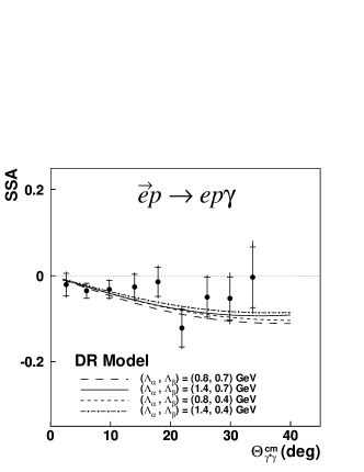
Figure 21: Beam single spin asymmetry (SSA) for VCS as function of the photon scattering angle. The dispersive predictions are shown for different pairs of ($\Lambda_{\alpha}$, $\Lambda_{\beta}$) given in GeV. Solid line: (1.4, 0.7), dashed-dotted line: (1.4, 0.4), long-dashed line: (0.8, 0.7), short-dashed line: (0.8, 0.4). Figure from Bensafa et al. (2007).

At larger virtuality, the VCS process has been investigated by the Hall A Collaboration at JLab, and data have been obtained at $Q^{2}=0.92$ GeV² and $Q^{2}=1.76$ GeV² Laveissiere et al. (2004). A reasonable description of these data is obtained by the values $\Lambda_{\alpha}=0.71$ GeV and $\Lambda_{\beta}=0.51$ GeV shown by the solid lines in Fig. 22. We note that $\Lambda_{\alpha}$ corresponds to a spatial range comparable to the nucleon’s charge distribution. However, the best fit value for $\Lambda_{\beta}$ is substantially lower, indicating that the diamagnetism is related to pion cloud effects at distances above 1 fm. Subtracting the spin-dependent terms according to the dispersion predictions, we obtain the $Q^{2}$ dependence of the scalar GPs shown in Fig. 23. It is obvious that the electric GP $\alpha_{E1}(Q^{2})$ is dominated by the asymptotic term, which however can not be described by a single dipole form over the full $Q^{2}$ range. The magnetic GP $\beta_{M1}(Q^{2})$ clearly shows a characteristic maximum at $Q^{2}~{}\approx 0.05$ GeV², which comes about by cancelation between the positive paramagnetic $\Delta$ contribution and the negative diamagnetic contribution of the $t$-channel $\pi\pi$ exchange. By Fourier transforming the GPs $\alpha_{E1}(Q^{2})$ and $\beta_{M1}(Q^{2})$ in the Breit frame, one obtains the spatial distribution of the induced electric polarization and magnetization of the nucleon L’vov et al. (2001). The emerging picture is as expected from a classical interpretation of diamagnetism. Due to the external magnetic field, pionic currents start circulating in the nucleon and give rise to an induced magnetization opposite to the applied field. At distances $r\gtrsim 1/m_{\pi}$, the diamagnetic effect dominates and the Fourier transform $\beta_{M1}(r)$ takes negative values, whereas the paramagnetic contributions prevail at the smaller distances giving rise to positive values of $\beta_{M1}(r)$ in the interior of the nucleon. As the momentum transfer $Q^{2}$ increases, the negative contribution due to the long-range pion cloud vanishes fast and hence $\beta_{M1}(Q^{2})$ increases. This nicely explains the positive slope of $\beta_{M1}(Q^{2})$ at $Q^{2}=0$ and the maximum at $Q^{2}\approx 0.05~{}\text{GeV}^{2}$ as indicated by the experimental data.

Figure 22: Results for $P_{LL}-P_{TT}/\varepsilon$ (left panel) and $P_{LT}$ (right panel). Dashed lines: dispersive $\pi N$ contributions. Dotted lines: asymptotic contributions with $\Lambda_{\alpha}=0.71$ GeV and $\Lambda_{\beta}=0.51$ GeV. Solid lines: full results. The data are from Olmos de Leon et al. (2001) (open triangles), Bourgeois et al. (2006) (full triangles), Roche et al. (2000) (squares), and Laveissiere et al. (2004) as obtained by the LEX (open circles) and DR (full circles) analysis. The inner error bars describe the statistical error, the outer error bars include systematical errors. Figure from Drechsel et al. (2003), updated by B. Pasquini.

Figure 23: Left panel: the electric GP $\alpha_{E1}(Q^{2})$ obtained from the DR formalism with $\Lambda_{\alpha}=0.7$ GeV (solid line) and $\Lambda_{\alpha}=1.79$ GeV (dashed-dotted line). The solid line is the sum of the asymptotic (dashed line) and dispersive (dotted) contributions. Right panel: the magnetic GP $\beta_{M1}(Q^{2})$ obtained from the DR formalism with $\Lambda_{\beta}=0.51$ GeV (solid line) and $\Lambda_{\beta}=0.63$ GeV (dashed-dotted line). The dashed-dotted line is the sum of the asymptotic (dashed line) and dispersive (dotted line) contributions. The data are from Olmos de Leon et al. (2001) (open triangles), Bourgeois et al. (2006) (full triangles), Roche et al. (2000) (squares), and Laveissiere et al. (2004) as obtained by the LEX (open circles) and DR (full circles) analysis. The inner error bars describe the statistical error, the outer error bars also include systematical errors. Figure from Laveissiere et al. (2004).

According to Eqs. (102) and (103), the unpolarized VCS experiment gives access to only 3 combinations of the 6 GPs. As was shown by Vanderhaeghen (1997), it takes experiments with polarized lepton beams and polarized targets or recoil nucleons to measure the remaining 3 GPs. These double-polarization observables require measuring the cross sections for a definite electron helicity $h$ and recoil (or target) proton spin orientation parallel and opposite to a specified axis. As shown for the unpolarized cross section by Eq. (101), also the polarized squared amplitude has a low-energy expansion, and again the GPs are obtained from the term $\mathcal{O}~{}(1)$. This term contains the structure functions $P_{LT}^{z}(q)$, $P_{LT}^{{}^{\prime}z}(q)$, and $P_{LT}^{{}^{\prime}\perp}(q)$, which are related to the spin GPs by Vanderhaeghen (1997)

$$P_{LT}^{z} = \frac{3Qq}{2\tilde{q}_{0}}G_{M}P^{(L1,L1)1}-\frac{3Mq}{Q}G_{E}P^{(M1,M1)1}\,,$$ (104)

$$P_{LT}^{{}^{\prime}z} = -\frac{3}{2}\,QG_{M}P^{(L1,L1)1}+\frac{3Mq^{2}}{Q\tilde{q}_{0}}\,G_{E}P^{(M1,M1)1}\,,$$

$$P_{LT}^{{}^{\prime}\perp} = \frac{3qQ}{2\tilde{q}_{0}}\,G_{M}\left(P^{(L1,L1)1}-\sqrt{\frac{3}{2}}\,\tilde{q}_{0}P^{(M1,L2)1}\right).$$

While $P_{LT}^{z}$ and $P_{LT}^{{}^{\prime}z}$ can be accessed by in-plane kinematics, $P_{LT}^{{}^{\prime}\perp}$ requires an out-of-plane measurement.

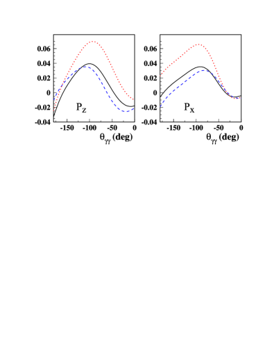
Figure 24: Predicted double-polarization asymmetries as function of the photon scattering angle $\theta_{\gamma\gamma}$ and for the following fixed kinematic values: $q=600~{}{\text{MeV}}$, $q^{\prime}=111.5~{}{\text{MeV}}$, $\varepsilon=0.62$, and $\Phi=0^{\circ}$. In order to highlight the model dependence, the (known) Bethe-Heitler and Born contributions to the asymmetry have been subtracted. Solid lines: Results of dispersion relations for $\Lambda_{\alpha}$ = 1 GeV and $\Lambda_{\beta}$ = 0.6 GeV Drechsel et al. (2003), dotted lines: predictions of HBChPT at $\mathcal{O}(p^{3})$ Hemmert et al. (2000), and dashed lines: HBChPT at $\mathcal{O}(p^{4})$ Kao et al. (2004). See text for further explanations.

In Fig. 24 we compare the results of DR and HBChPT for the double-polarization observables, with longitudinally polarized electrons and recoil proton polarization either along the virtual photon direction ($z$-direction) or in the reaction plane and perpendicular to the virtual photon ($x$-direction). The large but well-known asymmetries from the Bethe-Heitler and Born terms have been subtracted in this figure in order to highlight the differences between DR Pasquini et al. (2001a) and HBChPT at ${\mathcal{O}}(p^{3})$ Hemmert et al. (2000). We note that the latter approach yields significantly larger effects due to higher predicted values for the spin GPs. Although these double polarization observables are tough to measure, a first test experiment is underway at MAMI. Contrary to the scalar polarizabilities, the spin-flip GPs are still unknown territory. In Fig. 25 we compare the dispersive results for the spin-flip GPs with the predictions of the non-relativistic constituent quark model Pasquini et al. (2001b), the HBChPT to ${\mathcal{O}}(p^{3})$ Hemmert et al. (2000); Hemmert et al. (1997a) and ${\mathcal{O}}(p^{4})$ Kao and Vanderhaeghen (2002), and the linear $\sigma$-model Metz and Drechsel (1997). We refrain from commenting on the theoretical predictions which clearly open a wide range of values for the spin polarizabilities. An absolute must for further progress are dedicated experiments with a large sensitivity to the spin-dependent GPs. Such experiments are (I) unpolarized VCS with variation of the transverse photon polarization $\epsilon$ in order to separate the response functions $P_{LL}$ and $P_{TT}$ and (II) double-polarization experiments as discussed above.

Figure 25: The spin-flip GPs (without the $\pi^{0}$-pole contribution) from several calculations. Solid lines: dispersive $\pi N$ contribution Pasquini et al. (2001a), short-dashed lines: ${\mathcal{O}}(p^{3})$ HBChPT Hemmert et al. (2000), long-dashed lines: ${\mathcal{O}}(p^{4})$ HBChPT Kao et al. (2004), dashed-dotted lines: linear $\sigma$ model Metz and Drechsel (1996), dotted lines: non-relativistic CQM Pasquini et al. (2001b). For visibility, the tiny CQM results for $P^{(L1,L1)1}$ and $P^{(M1,L2)1}$ are multiplied by a factor 100. Figure from Drechsel et al. (2003) updated by B. Pasquini.

IV.3 Polarizability of mesons

Mesons are systems of a quark and an anti-quark and, therefore, theoretically simpler to describe than baryons. Let us set the scene with the classical picture of two charges bound in a quark-antiquark potential in the presence of an additional static electric field. For this system we can derive the following relation Walcher (2006):

$$\alpha^{\pi^{+}}_{E1}=\frac{\alpha_{em}}{\alpha_{q{\bar{q}}}}4\pi R^{3}\zeta^{2}\,,$$ (105)

with $\zeta=1/6$ the effective charge of the system and $\alpha_{q\bar{q}}\approx 5$ derived from the heavy quark potential, of course somewhat outside its applicability. Furthermore, $R$ is a characteristic dimension of the system, for example the equivalent charge radius. With the pion rms radius of Eq. (49), we obtain $R=\sqrt{(5/3)\langle r^{2}\rangle_{\pi}}=0.86$ fm, and as a result $\alpha^{\pi^{+}}_{E1}=3.2$, here and in the following in units of $10^{-4}~{}\text{fm}^{3}$. Comparing these numbers with the results of subsection IV.1, we find that the pion is a “dielectric medium” with $\varepsilon\approx 1.001$, i.e., even more rigid than the nucleon.

The pion polarizabilities have been calculated in ChPT at the two-loop order, ${\mathcal{O}}(p^{6}).$ Contrary to the situation of the nucleon, no “matter fields” with their own mass scale are present, and therefore the calculations can be performed in the original formulation of ChPT Gasser and Leutwyler (1984, 1985). This makes the following predictions for the polarizabilities a very significant test of this theory Gasser et al. (2006):

$$\alpha^{\pi^{+}}_{E1}+\beta^{\pi^{+}}_{M1} = 0.16\pm 0.1\,,$$ (106)

$$\alpha^{\pi^{+}}_{E1}-\beta^{\pi^{+}}_{M1} = 5.7\pm 1.0\,.$$ (107)

The very small value predicted by Eq. (106), that is Baldin’s sum rule applied to the pion, makes a measurement of this observable close to impossible. The experiments are therefore analyzed with the constraint $\alpha_{E1}^{\pi^{+}}\approx-\beta_{M1}^{\pi^{+}}$.

Unfortunately, the experimental situation is rather contradictory, see Ahrens et al. (2005) and Gasser et al. (2006) for recent reviews of the data and further references to the experiments. There exist basically three different methods to measure $\alpha_{E1}$: (I) the reactions $e^{+}e^{-}\rightleftarrows\gamma\gamma\rightleftarrows\pi^{+}\pi^{-}$, (II) the Primakov effect of scattering a relativistic pion in the Coulomb field of a heavy nucleus, and (III) the radiative pion photoproduction, $p(\gamma,\gamma^{\prime}\pi^{+}n)$, which contains Compton scattering on a (bound) pion as a subprocess. The latter reaction was recently investigated at the Mainz Microtron MAMI, by use of a kinematically optimized set-up consisting of the backward photon detector TAPS, a forward $\pi^{+}$ detector, and a neutron detector realized by a large scintillator wall of dimensions 3x3x0.5 m³. The largest error of this measurement is due to the systematic error of the neutron efficiency. The final result of the experiment is Ahrens et al. (2005)

$$\alpha^{\pi^{+}}_{E1}-\beta^{\pi^{+}}_{M1}=11.6\pm 1.5_{\text{stat}}\pm 3.0_{\text{syst}}\pm 0.5_{\text{mod}}\,,$$ (108)

which is at variance with the prediction of Gasser et al. (2006) by two standard deviations. In view of the theoretical uncertainties from the fact that the Compton scattering is off a bound pion, the deviation from theory is an open problem. In particular we point out that the model error in Eq. (108) is estimated by comparing the analysis with 2 specific models. This does not exclude that a wider range of models will lead to a larger model error. Considering the fact that the scattering is off a “constituent” pion in the nucleon, we may attribute the deviation to binding effects. For example, as suggested by Eq. (105), an increase of the bound pion radius by 20 % would give a hand-waving explanation for the experimental data. Because the pion polarizability is extremely important for our understanding of QCD in the confinement region, it is prerequisite to check the given arguments by a full-fledged ChPT calculation of the reaction $p(\gamma,\gamma^{\prime}\pi^{+}n)$ .

The second method to determine the polarizability, the Primakov effect, has been studied at Serpukhov with the result

$$\alpha^{\pi^{+}}_{E1}-\beta^{\pi^{+}}_{M1}=13.6\pm 2.8_{\text{stat}}\pm 2.4_{\text{syst}}\,,$$ (109)

in agreement with the value from MAMI. Recently, also the COMPASS Collaboration at CERN has investigated this reaction. However, at this time the analysis is still in a too preliminary stage to include the result. Unfortunately, the reactions $e^{+}e^{-}\rightleftarrows\gamma\gamma\rightleftarrows\pi^{+}\pi^{-}$ have led to even more contradictory results in the range $4.4\leq\alpha^{\pi^{+}}_{E1}\leq 52.6$, as listed in the work of Gasser et al. (2006). In conclusion one has to wait for an improved analysis and possibly also independent experimental efforts before final conclusions can be drawn.

V Excitation spectrum of the Nucleon

V.1 Threshold production of mesons

As outlined in subsection II.4, the threshold photoproduction of mesons provides a significant test of our theoretical understanding, because only few partial waves contribute and, therefore, all relevant multipoles can be directly determined by the experiment. The case of neutral pion photoproduction on the proton, $\gamma(q)+p(p_{1})\rightarrow\pi^{0}(k)+p(p_{2})$ is of particular interest. For the s-wave threshold multipole $E_{0+}$ of this reaction, several authors had derived a low energy theorem (LET) based on current algebra and PCAC De Baenst (1970); Vainshtein and Zakharov (1972). According to the theorem, the leading terms of the threshold multipole were directly determined by the Born diagrams, evaluated with the pseudovector pion-nucleon interaction. However, this prediction had to be revised in the light of surprising experimental evidence. The reason for the discrepancy between the theorem and the data was first explained in the framework of ChPT by pion-loop corrections. An expansion in the mass ratio $\mu=m_{\pi}/M\approx 1/7$ yielded the result Bernard et al. (1991a)

$$E_{0+}(\pi^{0}p)=\frac{eg_{\pi N}}{8\pi m_{\pi}}\left\{\mu-\mu^{2}\,\frac{3+\kappa_{p}}{2}-\mu^{2}\,\frac{M^{2}}{16f^{2}_{\pi}}+\ ...\right\}\ ,$$ (110)

where $g_{\pi N}$ is the pion-nucleon coupling constant and $f_{\pi}\approx 93$ MeV the pion decay constant. We observe that $E_{0+}(\pi^{0}p)$ is proportional to $\mu$, which suppresses this reaction relative to charged pion production. The first and the second term on the rhs of Eq. (110) are identical to the “LET” of De Baenst (1970) and Vainshtein and Zakharov (1972), which however has to be corrected by the third term on the rhs. Although this loop correction is formally of higher order in $\mu$, its numerical value is of the same size as the leading term.

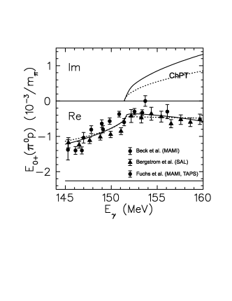
Figure 26: The real (Re) and imaginary (Im) parts of the s-wave amplitude $E_{0+}$ for $\pi^{0}$ photoproduction at threshold energies. The MAMI data of Beck et al. (1990) and Fuchs et al. (1996) are represented by circles, the SAL data of Bergstrom et al. (1996) by triangles. Dashed lines: predictions of ChPT at ${\cal{O}}$($p^{3}$) Bernard et al. (1996b, a), solid lines: results from dispersion relations Hanstein et al. (1997). The solid horizontal line at about -2.2 shows the prediction of De Baenst (1970) and Vainshtein and Zakharov (1972). Figure by courtesy of R. Beck.

The energy dependence of $E_{0+}(\pi^{0}p)$ is shown in Fig. 26. The discrepancy between predictions of De Baenst (1970) and Vainshtein and Zakharov (1972) and the experimental data obtained at the Mainz Microtron MAMI and at SAL (Saskatoon) is apparent. Furthermore, the real part of the amplitude shows a characteristic “Wigner cusp” at the threshold for charged pion production, which lies about 5 MeV above the $\pi^{0}$ threshold. This cusp in the real part is related to the sharp rise of the imaginary part at the second threshold. The physical picture behind the large loop correction is based on (I) the high production rate of charged pions and (II) the charge-exchange scattering between the nucleon and the slow $\pi^{+}$ in the intermediate state, which leaves a $\pi^{0}$ in the final state. However, the direct experimental determination of the imaginary part will require double-polarization experiments with linearly polarized photons and polarized targets. The excellent agreement between ChPT and the data for $E_{0+}$ is somewhat flawed by the fact that higher order diagrams are sizeable, that is, the perturbative series converges slowly and low-energy constants appearing at the higher orders reduce the predictive power.

For a more quantitative presentation of the results, the $E_{0+}$ amplitude was parameterized as the sum of a direct and a charge-exchange term Bernstein et al. (1997),

$$E_{0+}(\pi^{0}p) = A_{0}(q)+i\,a_{\pi^{+}\pi^{0}}\,A_{+}k_{\pi^{+}}$$ (111)

$$= A_{0}(q)+i\,\beta\,k_{\pi^{+}}\,,$$ (112)

with $A_{0}(q)=a_{0}+a_{1}(q-q_{\text{thr}})$ and $A_{+}$ describing the neutral and charged pion production in the absence of the charge exchange reaction, $a_{\pi^{+}\pi^{0}}$ the scattering length for charge exchange, and $k_{\pi^{+}}$ the momentum of the charged pion appearing in the intermediate state. This leaves the 3 fit parameters $a_{0}$, $a_{1}$, and $\beta$ in oder to determine the s wave. As discussed in subsection II.4, the unpolarized cross section gives information on only 2 of the 3 p-wave amplitudes. A complete experiment therefore requires measuring a further observable, e.g., the photon asymmetry $\Sigma$ of Eq. (26). The result obtained at MAMI is depicted in Fig. 27.

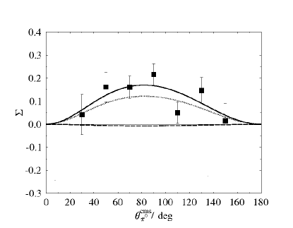
Figure 27: The angular distribution of the photon asymmetry $\Sigma$ for the reaction $p(\vec{\gamma},\pi^{0})p$. Dashed line: results of dispersion relations Hanstein et al. (1997), dotted line: prediction of ChPT Bernard et al. (1996b), full line: empirical fit to the data with Eqs. (25) and (26). Figure from Schmidt et al. (2001).

The data of Schmidt et al. (2001) for the s- and p-wave amplitudes are compared to the results of ChPT and dispersion relations in Table 1. The predictions of ChPT for the p waves are in good agreement with the data, whereas $P_{3}$ comes out much too small in dispersion theory. Since the latter approach is mainly based on input from the imaginary parts of the multipoles $M_{1+}$ and $M_{1-}$ in the resonance region, this failure may indicate that even the structure of the low-lying resonances $\Delta(1232)$ and $N^{\ast}(1440)$ is not yet completely unraveled.

	Schmidt et al. (2001)	ChPT	DR
$E_{0+}(\pi^{0})$	$-1.23\pm 0.08\pm 0.03$	-1.16	-1.22
$E_{0+}(\pi^{+})$	$-0.45\pm 0.07\pm 0.02$	-0.43	-0.56
$\beta$	$2.43\pm 0.28\pm 1.0$	2.78	3.6
$P_{1}$	$9.46\pm 0.05\pm 0.28$	$9.14\pm 0.5$	9.55
$P_{2}$	$-9.5\pm 0.09\pm 0.28$	$-9.7\pm 0.5$	-10.37
$P_{3}$	$11.32\pm 0.11\pm 0.34$	$10.36$	9.27
$P_{23}$	$10.45\pm 0.07$	11.07	9.84

Table 1: Experimental results of Schmidt et al. (2001) for $E_{0+}(\pi^{0}p)$ at the $\pi^{0}$ and $\pi^{+}$thresholds in units of $10^{-3}/m_{\pi^{+}}$, four combinations of the (reduced) $P$-wave amplitudes in units $k\cdot 10^{-3}/m_{\pi^{+}}^{2}$, and the parameter $\beta$ (with statistical and systematic errors, in order) compared to the predictions of ChPT Bernard et al. (1996b, a) and dispersion relations (DR) Hanstein et al. (1997). For the definition of the reduced $P$-wave amplitudes see section II.4.

Figure 28: The total cross section for the $p(e,e^{\prime}p)\pi^{0}$ reaction as function of $Q^{2}$ for several values of the excitation energy $\Delta W=W-M-m_{\pi^{0}}$. The data at $Q^{2}=0.05$ GeV² and $0.10$ GeV² are from Merkel et al. (2002) and Distler et al. (1998), respectively. The solid line represents the prediction of ChPT Bernard et al. (1996c) and the dashed line the result of the phenomenological model MAID Drechsel et al. (1999). Figure from Merkel et al. (2002).

Figure 29: The separated cross sections $\sigma_{0}$, $\sigma_{LT}$, and $\sigma_{TT}$ as well as the beam helicity asymmetry $A_{LT}^{\prime}$ at $\theta_{\pi}^{\ast}=90^{\circ}$. Solid line: HBChPT Bernard et al. (1996c), dashed line: MAID Drechsel et al. (1999), dashed-dotted line: DMT model Kamalov et al. (2001). Figure from Weis et al. (2007).

The great success of ChPT for photoproduction at threshold was a strong motivation to extend the experimental program to electroproduction. Because the virtual photon has an additional longitudinal component, 3 more partial waves appear to leading order: the longitudinal s-wave amplitude $L_{0+}$ and the p-wave amplitudes $L_{1+}$ and $L_{1-}$, describing the excitation of the $\Delta(1232)$) and $N^{\ast}(1440)$, respectively. Moreover, all the amplitudes are functions of $Q^{2}$, that is, they probe the spatial distribution of pion production on the nucleon. The first investigations performed at NIKHEF van den Brink et al. (1995) and MAMI Distler et al. (1998) for $Q^{2}=0.10~{}\text{GeV}^{2}$ provided another confirmation of ChPT although at the expense of 2 new low-energy constants, which were fitted to the data. In order to further check this agreement, data were also taken at the lower momentum transfer $Q^{2}=0.05~{}\text{GeV}^{2}$ Merkel et al. (2002). The total cross section obtained by these measurements is compared with the predictions of ChPT in Fig. 28, which shows the total cross sections near threshold as function of $Q^{2}$. The comparison was made on the basis of the total cross sections in order to eliminate all possible systematic and model errors connected with the separation in longitudinal and transverse parts. It is apparent that the $Q^{2}$ dependence of the data can not not be fully described by theory. We consider this an important issue that deserves further investigations.

We conclude this subsection by presenting some recent results of Weis et al. (2007). Whereas former experiments were only sensitive to the real part of the amplitudes, these authors also determined the fifth structure function ($LT^{\prime}$) given in Eq. (II.4). This function can only be measured with polarized electrons and out-of-plane, i.e., for finite values of the pion azimuthal angle with regard to the electron scattering plane. Furthermore, its multipole decomposition is of the form Im $(L_{0+}^{\ast}\,M_{1+}+\cdots)$, i.e., this function contains information on the phase of the s-wave amplitude. With the shorthand notation $d\sigma_{i}/d\Omega_{\pi}^{\ast}\equiv\sigma_{i}$, Weis et al. (2007) separated the partial cross sections $\sigma_{0}=\sigma_{T}+\varepsilon\sigma_{L}$, $\sigma_{TT}$, and $\sigma_{LT}$ as well as the beam asymmetry $A_{LT}^{\prime}$ corresponding to $\sigma_{LT}^{\prime}$. The result is displayed in Fig. 29. We observe that only the dynamical Dubna-Mainz-Taipei (DMT) model Kamalov et al. (2001) is able to fully describe the experiment, in particular its prediction for the helicity asymmetry is right on top of the data. Such dynamical models start from a description of the pion-nucleon scattering phases by a quasi-potential, which serves as input for an integral equation to account for multiple scattering. In this sense the model contains the loop corrections to an arbitrary number of rescattering processes, and is therefore perfectly unitary, albeit on a phenomenological basis that may violate gauge invariance to some extent.

V.2 Nucleon resonances and meson production

The total photoabsorption cross section $\sigma_{T}$ for the proton is displayed in Fig. 30. It clearly exhibits 3 broad resonance structures on top of a strong background. These structures correspond, in order, to magnetic dipole $(M1)$ excitation of the $\Delta(1232)$ resonance, electric dipole $(E1)$ strength near the resonances $N^{\ast}(1520)$ and $N^{\ast}(1535)$, and electric quadrupole $(E2)$ strength near the $N^{\ast}(1680)$. The figure also shows the contributions of the most important channels: the one-pion channels dominate up to $\nu\approx 500$ MeV, the two-pion branching ratio becomes comparable in the second resonance region at $\nu\approx 700$ MeV, and the large $\eta$ branch of the resonance $N^{\ast}(1535)$ is hidden in the background. Because the nucleon resonances lie above the one-pion threshold, any separation in a continuous background and discrete resonances is necessarily model-dependent. In particular, because background and resonance contributions interfere, a careful analysis of the partial waves and their relative phases is mandatory. Figure 31 depicts the partial cross sections for the different decay channels investigated so far. The rapid increase of the two-pion contribution between 400 and 600 MeV is clearly seen, from whereon it provides more than half of the total absorption. Another interesting feature is the dominance of charged pion production both below and above the $\Delta(1232)$ resonance. Finally, one notes the small $\eta$ decay branch, which corresponds to s-wave $\eta$ production mediated by the $S_{11}(1535)$.

Figure 30: The total photoabsorption cross section $\sigma_{T}$ on the proton as function of the photon lab energy $\nu$ . The various lines represent the MAID results Drechsel et al. (1999) for the total cross section (solid line), one-pion channels (dashed line), more-pion channels (dashed-dotted line), and $\eta$ channel (dotted line). Full circles: total cross section from MAMI MacCormick et al. (1996), open circles: data from Daresbury Armstrong et al. (1972), open triangles: two-pion production Braghieri et al. (1995). Figure by courtesy of J. Ahrens.

Figure 31: The partial and total cross sections for the absorption of photons on the proton as a function of the photon lab energy $\nu$ obtained at MAMI. Open circles: total cross section as in Fig. 30 MacCormick et al. (1996), solid and open triangles: $n\pi^{+}$ decay channel MacCormick et al. (1996), open diamonds: $p\pi^{0}$ decay channel MacCormick et al. (1996), asterisks: two-pion production Braghieri et al. (1995), open squares: $p\eta$ channel Krusche et al. (1995). Figure by courtesy of J. Ahrens.

In the past, the primary method to unravel the nucleon resonance spectrum were experiments with strong interactions, in particular pion-nucleon scattering. These data have been systematically studied by the Karlsruhe group Höhler (1983); Koch (1985) and the GWU Collaboration using the code SAID Arndt et al. (2002, 2004, 2006). A summary of the known spectroscopic information on nucleon resonances is given by the Particle Data Group (PDG) Yao et al. (2006). It is the objective of these studies to determine the relevant characteristics of the resonances, their pole positions, widths, decay channels, and branching ratios. In a first step, the full data base is fitted within the framework of a partial wave analysis. If a particular partial wave shows some rapid increase of the scattering phase over a limited energy region, the fit is then repeated with a form containing both a smooth background and a resonance form, mostly of the Breit-Wigner shape. Because of the strong decay channels and large resonance widths of typically 100 MeV and more, the ideal resonance form is only realized for the first resonance, the $\Delta(1232)$: the pion-nucleon scattering phase $\delta_{33}(W)$ goes through $90^{\circ}$, the real part of the multipole vanishes, and the imaginary part has a maximum near $W=M_{R}\approx 1232~{}$MeV. Because of inelastic channels, overlapping resonances, and energy-dependent backgrounds, these conditions are not fulfilled by the higher resonances. A mere “bump” in a partial wave is not necessarily a resonance, it may also originate from the opening of a new channel, which usually produces an asymmetric resonance shape. The “speed-plot” technique is particularly useful to probe the resonance structure. It requires the derivative of the partial wave amplitude with regard to the energy $W$, which is then compared to the corresponding derivative of an ideal Breit-Wigner resonance. In this way one determines the pole position and the residue of the multipole in the complex energy plane, which are unique characteristics of a resonance.

Figure 32: Resonance contributions to the total photoabsorption cross section of the proton. The calculations are from the unitary isobar model MAID2003 Drechsel et al. (1999). Figure by courtesy of R. Beck and L. Tiator.

Because the cross sections for electroexcitation are suppressed by the fine structure constant $\alpha_{\text{em}}$, systematic studies of the resonance structure were only possible after the advent of the new electron accelerators providing high duty-cycle and flux density of photons and electrons. The virtues of these investigations are obvious: the selectivity through transverse electric and magnetic as well as longitudinal photon fields allows for the separation of multipoles and investigations of the spin degrees of freedom, the study of specific final states with different mesons by coincidence experiments, and the possibility to resolve the spatial distribution of charge and current densities by varying the virtuality of the photon. Figure 32 sets the scene by showing the individual contributions of the main nucleon resonances to the total photoabsorption cross section. The resonances in the figure are labeled in the spectroscopic notation, see subsection II.5. As an example, the $\Delta(1232)=P_{33}(1232)$ has the pion in a p wave and both isospin and spin are 3/2. As is evident from Fig. 32, the $\Delta(1232)$ is the dominant feature in the resonance spectrum. It contributes more than 400 $\mu$b at the maximum of the absorption cross section. Already in the second resonance region, there are several overlapping resonances, the small Roper resonance $P_{11}(1440)$ with the same quantum numbers as the nucleon, as well as the relatively strong $D_{13}(1520)$ and the weaker $S_{11}(1535)$, both mainly excited by electric dipole radiation, all on top of a large background (not shown in the figure!) and on the tails of the neighboring resonances. In the third resonance region, the figure shows only the dominant $F_{15}(1680)$ resonance with a concentration of the electric quadrupole strength. The number of known (and unknown) resonances increases in the higher part of the spectrum, see Yao et al. (2006). However, somewhere above $W\approx 1.5$ GeV the notion of “resonances” becomes problematic and has to be replaced by a continuum which, of course, can be expanded in partial waves as discussed in subsection II.5. The problem is clearly not on the experimental side, but in the modeling of the spectrum, which for $W\geq 1.5$ GeV should be based on coupled channel calculations. As has been mentioned before, the most valid technique is the “speed plot” Höhler (1983), which gives information about the resonance position in the complex energy plane. However, the distinction of “resonances” and “background” becomes increasingly difficult, and looses its meaning for energies somewhere above 2 GeV. The “missing resonances” issue of the constituent quark model (CQM) that predicts more resonances than have been observed Isgur and Karl (1979); Metsch et al. (2003), may disappear in view of the “resonance-background” problem Thoma (2005).

As in the case of the elastic form factors discussed in section III, the $Q^{2}$ dependence of the multipole transitions provides information on the spatial distribution of these observables. Let us discuss this issue for the $\Delta(1232)$. The 3 (real) transition form factors $G_{M}^{\ast}$, $G_{E}^{\ast}$, and $G_{C}^{\ast}$ are related to the (complex) partial wave amplitudes according to Eq. (30). The magnetic dipole transition $M_{1+}$ dominates, the electric and Coulomb quadrupole transitions $E_{1+}$ and $S_{1+}$ are much smaller. A finite value of the quadrupole moment requires that the wave functions of either the nucleon or the $\Delta(1232)$, or most likely both are deformed. In the CQM, such a deformation follows from the tensor force contained in the color-hyperfine interaction among the quarks De Rujula et al. (1975); Isgur et al. (1982); Capstick and Karl (1990). However, typical CQM calculations Capstick and Keister (1995); De Sanctis et al. (2005b) underestimate the electric and Coulomb quadrupole amplitudes $E_{1+}$ and $S_{1+}$. In models with pionic degrees of freedom, the deformation arises naturally from the spin-dependent coupling of the pion to the quarks. The pions have been introduced in several approaches, such as chiral bag models Vento et al. (1980); Bermuth et al. (1988); Lu et al. (1997), dynamical models Sato and Lee (2001); Kamalov and Yang (1999), and effective field theories Pascalutsa and Vanderhaeghen (2005, 2006); Gail and Hemmert (2006). Although differing considerably in the details, all these models describe the experimental data reasonably well. In particular the chiral effective field theories (EFTs) are based on a systematic expansion in terms of the external momenta, the pion mass, and the N$\Delta$ mass splitting. Contrary to the dynamical models they are gauge and Lorentz invariant, however, being based on a perturbative expansion, the unitarity condition is only approximately fulfilled.

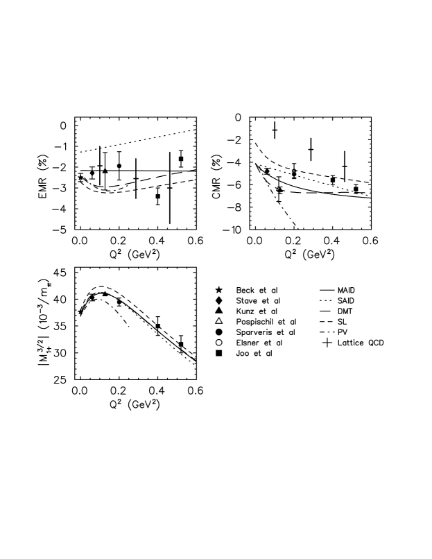
Figure 33: The ratios EMR=$R_{EM}$ and CMR=$R_{EM}$ together with the amplitude $M^{3/2}_{1+}$ of the N$\Delta(1232)$ transition as function of $Q^{2}$. The data are from Beck et al. (2000) (asterisks), Stave et al. (2006) (diamonds), Kunz et al. (2003) (solid triangles), Pospischil et al. (2001) (open triangles), Sparveris et al. (2006) (solid circles), Elsner et al. (2006) (open circles), and Joo et al. (2004) (squares). The theoretical predictions are represented by solid lines: MAID2007 Drechsel et al. (2007), dotted lines: SAID Arndt et al. (2002), long-dashed lines: DMT Kamalov and Yang (1999), short-dashed lines: Sato-Lee model Sato and Lee (2001), dot-dashed lines: ChEFT Pascalutsa and Vanderhaeghen (2005, 2006), and crosses: predictions with error bars from Lattice QCD Alexandrou et al. (2005). Figure adapted from Sparveris et al. (2006) by L. Tiator.

Of course, the deformation can not be measured for the nucleon ground state, because the intrinsic static quadrupole moment $Q_{0}$ and the observed quadrupole moment are related by $Q^{\text{obs}}_{J}=[3\langle M\rangle^{2}-J(J+1)]/[J(2J-1)]\,Q_{0}$. This rule allows one to observe the quadrupole moment of the $\Delta(1232)$ but, of course, the highly unstable $\Delta(1232)$ can not serve as a static target. Therefore, the deformation issue can only be accessed through the electromagnetic transitions from the nucleon to the $\Delta(1232)$. In the following we discuss the ratios of the multipole transitions at the resonance position, $R_{EM}$ and $R_{SM}$ as defined by Eq. (33). We repeat that the resonance position of the $\Delta(1232)$ is uniquely defined within the validity of the Fermi-Watson theorem, that is, (I) the real parts of all 3 N$\Delta$ amplitudes vanish at $W=M_{\Delta}$, because all the amplitudes carry the same phase, namely the pion-nucleon phase shift in the partial wave with $\ell=1$ and $I\,=\,J=\,\frac{3}{2}$, $\delta_{33}(W)$.

Many experimental and theoretical investigations have been devoted to the N$\Delta$ transition with real photons, for a summary of this work see Beck (2006). The most precise value for the ratio of the multipoles,

$$R_{EM}=(-2.4\pm 0.16_{\text{stat}}\pm 0.24_{\text{syst}})\%\,,$$ (113)

was obtained with linearly polarized photons Beck et al. (2000); Leukel (2001). These authors also studied neutral and charged pion production on the proton, which is necessary to isolate the isospin $\frac{3}{2}$ amplitude relevant for the N$\Delta$ transition. At finite $Q^{2}$ the same physics questions were addressed by pion electroproduction, $e+p\rightarrow e^{\prime}+p^{\prime}+\pi^{0}$, measuring the scattered electron in coincidence with the recoil proton detected in a high-resolution magnetic spectrometer. The small solid angle of these instruments does not limit the accuracy since the protons are focused by the relativistic boost along $\vec{q}$. Such experiments were first performed at MIT/Bates Mertz et al. (2001) and then extended by Sparveris et al. (2005) to out-of-plane angles with the OOPS spectrometer. This work was continued in the framework of the A1 Collaboration at MAMI/Mainz Sparveris et al. (2006); Elsner et al. (2006); Stave et al. (2006). In particular, Stave et al. (2006) also measured the structure function $\sigma^{\prime}_{LT}$ by use of polarized electrons and out-of-plane proton detection. The experimental results for the $\Delta$ multipoles in the low-$Q^{2}$ region are compared to several model calculations in Fig. 33. We observe that the leading multipole $M_{1+}$ is described quite well by the models. It is also also worthwhile mentioning that the dynamic models ascribe a third of the magnetic dipole strength to the pion cloud. The predictions scatter much more with regard to the quadrupole strength as shown by the ratios $R_{EM}$ and $R_{SM}$. Concerning the origin of “deformation”, both the dynamic models Sato and Lee (2001); Kamalov and Yang (1999) and effective field theory Pascalutsa and Vanderhaeghen (2005, 2006); Gail and Hemmert (2006) agree that the multipoles $E_{1+}$ and $S_{1+}$ are essentially due to the pion cloud. For a detailed comparison of these models in the $\Delta$ region, see Drechsel and Tiator (2007).

In many of the mentioned contributions, the authors have pointed out a considerable model-dependence of the analysis. It is therefore a substantial progress in this field that Kelly et al. (2007) performed a series of double-polarization experiments at $Q^{2}=1$ GeV² near the $\Delta$ region. Altogether they extracted 16 of the 18 independent response functions, most of them for the first time. As mentioned before, the experimental cross section is obtained by summing bilinear products of multipole amplitudes, $\sum_{\ell,\ell^{\prime}}{\mathcal{M}}^{\ast}_{\ell}{\mathcal{M}}_{\ell^{\prime}}$. Whereas the unpolarized response functions or cross sections, in shorthand $\sigma_{T}$, $\sigma_{L}$, $\sigma_{TT}$, and $\sigma_{LT}$ are obtained from the real parts of these products, many of the polarized cross sections are given by the imaginary parts, the first example being the “fifth structure function” $\sigma_{LT}^{\prime}$ measured with polarized beams. Because the N$\Delta$ multipoles carry the same phase, their product can only contribute to responses built from the real parts. On the other hand, the responses containing the imaginary parts yield information on the interference between the N$\Delta$ and background multipoles. The findings of Kelly et al. (2007) can be summarized as follows: (I) response functions governed by real parts are in general agreement with recent model calculations, (II) response functions determined by imaginary parts may differ substantially from the experiment and among the calculations, (III) the multipole analysis yields better results than a (truncated) Legendre series, and (IV) the model builders should go back to the drawing board to get better control of the non-resonant background, in particular at the larger virtualities $Q^{2}$.

As mentioned above, the typical CQM calculations underestimate the $\Delta$ multipoles, in particular the electric and longitudinal ones. Therefore, any successful description of these observables needs a pion cloud, at least if one insists on a reasonable size of the quark bag. Such descriptions are the chiral bag models, the dynamical models, and effective field theories. Taking all facts together, one is again forced to accept the dominant role that pions play for the structure of the nucleon. Of special interest is the recent work to solve QCD on the space-time lattice. Since these calculations can not yet be performed at the small (current) quark masses corresponding to the physical pion mass, one uses very large quark masses leading to pion masses $m_{\pi}\gtrsim 300$ MeV. The results are then extrapolated to the physical pion mass by extrapolating functions, ideally as derived from chiral effective field theories. Such procedure is not undisputed because the chiral expansion is hardly valid at pion masses much larger than the physical mass. However, the chiral extrapolation shows that unexpected phenomena occur when the pion mass is lowered from a few hundred MeV to its physical value: near the pion mass value for which the $\Delta$ resonance can decay, the chiral extrapolation becomes non-analytic, which leads to a kink and strong curvature in the extrapolation formula Pascalutsa et al. (2007).

As a further instructive example we present some results for the electroproduction of $\eta$ mesons, which are mainly produced by the decay of the $S_{11}(1535)$ resonance with $J=I=\frac{1}{2},\,\ell=0$. As is evident from Fig. 31, the $S_{11}(1535)$ is buried under the total cross section. However it is clearly seen in the $\eta$ channel, because this resonance has an $\eta$ branching ratio of 45-60% compared to a few per cent for other excitations of the nucleon Vrana et al. (2000). Eta photoproduction experiments at threshold show a strong increase of the cross section in the range of the resonance and an s-wave angular distribution in agreement with the given assignment Krusche et al. (1995). However, the shape of the resonance is very asymmetric, and also the speed-plot analysis does not yield satisfactory solutions Höhler (1993). Because of this unusual behavior several alternative interpretations have been given, for example in terms of a K$\Sigma$ molecular state Kaiser et al. (1997). Also the helicity amplitude $A_{1/2}$ of this resonance has an unusually soft form factor, as displayed in Fig. 34 for the $p(e,e^{\prime}p)\eta$ reaction measured at the Jefferson Lab Denizli et al. (2007).

Figure 34: The helicity amplitude $A_{1/2}$ for the $S_{11}(1535)$ in the $p(e,e^{\prime}p)\eta$ reaction. The data are represented by filled circles: Denizli et al. (2007), crosses: Armstrong et al. (1999), and open circles: earlier publications as specified by Denizli et al. (2007). The predictions are based on quark models and given by the solid line Capstick and Keister (1995) and the dotted line Aiello et al. (1998). Figure from Denizli et al. (2007).

It is striking how flat this transition form factor stays compared to the typical dipole form for other form factors of the nucleon. We further notice that the constituent quark model calculations, relativistic or not, can not fully explain the slow falloff with $Q^{2}$. It is also tempting to identify the structure near $Q^{2}\approx 0.2~{}\text{GeV}^{2}$ with a meson cloud effect as discussed in section III.1.

Another small but interesting resonance in the second resonance region is the Roper resonance $P_{11}(1440)$ with the same quantum numbers as the nucleon. The CQM describes this resonance by a radial excitation of the nucleon, and therefore it should be sensitive to the radial form of the bag potential. However, its mass is much lower than expected in simple quark models. Li et al. (1992) suggested that the Roper could also be a quark-gluon hybrid state, which, however, can not be excited by the longitudinal current or Coulomb field. Recent data on the electroproduction of this resonance are shown in Fig. 35 and compared with the single-energy and global solutions of MAID2007. We note that the amplitude $A_{1/2}$ (magnetic dipole transition) has a zero crossing at small momentum transfer. Furthermore, the amplitude $S_{1/2}$ (Coulomb monopole transition) rises to quite large values, which rules out the quark-gluon hybrid model.

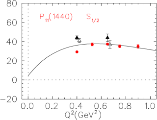
Figure 35: The helicity amplitudes $A_{1/2}$ and $S_{1/2}$ of the $P_{11}(1440)$ as function of $Q^{2}$. The triangles are from the analysis of Aznauryan et al. (2005) based on data of the CLAS Collaboration at JLab and obtained from dispersion relations (open triangles) and the unitary isobar model (filled triangles). The solid line is the global solution of MAID2007 Drechsel et al. (2007), a fit to the full data basis, and the filled circles are local fits to the data in the particular energy region. The data point at $Q^{2}=0$ is from the PDG Yao et al. (2006). Figures from Drechsel et al. (2007).

In section VI we also discuss the helicity structure of the second and third resonance regions with regard to several sum rules for real and virtual photons. However, with increasing excitation energy it becomes more and more difficult to isolate individual resonances by inclusive cross sections. It will therefore take a full-fledged program with polarized beams and targets as well as recoil polarization to analyze the higher mass region and to identify resonance structures on top of the large background.

VI Sum rules

The persisting problem of gaining a quantitative understanding of nucleon structure is one of the reasons why we are interested in sum rules. Being based on quite general principles like causality, unitarity, Lorentz and gauge invariance, sum rules should be valid for every model or theory respecting these principles and having a “reasonable” high-energy behavior. Therefore, the agreement or disagreement between theoretical predictions and the sum rule provides invaluable information on the quality of the approximations involved and whether or not the relevant degrees of freedom have been included. Specifically, if we compare a sum rule value with accurate experimental data up to a certain maximum energy, we learn whether the physics responsible for the sum rule is provided by the phenomena up to that energy, or whether possibly new degrees of freedom come into the game. As an example, Baldin’s sum rule relates the forward scalar polarizability to an energy-weighted integral over the total photoabsorption cross section and thus allows for an independent check of the results from Compton scattering. Moreover, recent double-polarization experiments have determined the helicity structure of this cross section for the proton. From these data, the forward spin polarizability has been obtained, and the Gerasimov-Drell-Hearn (GDH) sum rule has been verified within the experimental error bars of less than 10 %. Data have also been taken for the neutron and are under evaluation. With some caveat in mind, these sum rules can be generalized to the scattering of virtual photons. The integrands of the respective integrals are related to the electroexcitation cross sections and, in the limit of deep inelastic scattering (DIS), to the nucleon structure functions. The resulting generalized integrals and polarizabilities depend on the photon’s 4-momentum and therefore contain information on the spatial distribution of these observables.

VI.1 Sum rules for real photons

VI.1.1 Forward dispersion relations and sum rules

The forward scattering amplitudes $f$ and $g$ of Eqs. (61) - (63) can be determined by scattering circularly polarized photons (helicity $\lambda=\pm 1$) off nucleon targets that are polarized along or opposite to the photon momentum $\vec{q}$ as shown schematically in Fig. 36. If the spins are parallel, the helicity of the intermediate hadronic state takes the value $\textstyle{\frac{3}{2}}$. Since this requires a total spin $J\geq\textstyle{\frac{3}{2}}$, the transition can only take place on a correlated 3-quark system. For opposite spins, on the other hand, the helicity is conserved and the scattering can also take place on an individual quark. Denoting the Compton scattering amplitudes for these two experiments by $T_{3/2}$ and $T_{1/2}$, we find $f(\nu)=\textstyle{\frac{1}{2}}(T_{1/2}+T_{3/2})$ and $g(\nu)=\textstyle{\frac{1}{2}}(T_{1/2}-T_{3/2})$. Furthermore, the total absorption cross section is given by the spin average over the helicity cross sections,

$$\sigma_{T}=\frac{1}{2}\,(\sigma_{1/2}+\sigma_{3/2})\ ,$$ (114)

and the helicity-dependent cross section by the helicity difference,

$$\sigma_{TT}=\frac{1}{2}\,(\sigma_{1/2}-\sigma_{3/2})\ .$$ (115)

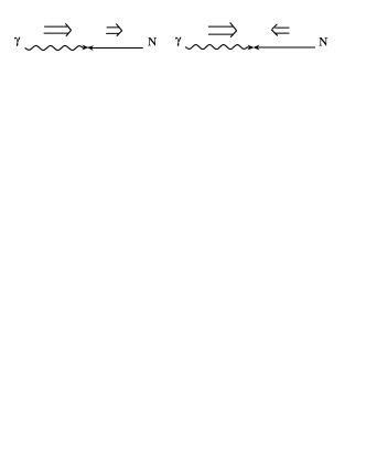
Figure 36: Spins and helicities in the reaction $\vec{\gamma}+\vec{N}\rightarrow N^{\ast}$. The open arrows denote the projections of the spin on the photon momentum, $S_{z}$, the helicities $h$ are the projections on the respective particle momentum, and the photon has right-handed helicity, $\lambda=+1$.
Left: $N(S_{z}=1/2,\ h=-1/2)\rightarrow N^{\ast}(S_{z}=h=3/2)$,
right: $N(S_{z}=-1/2,\ h=1/2)\rightarrow N^{\ast}(S_{z}=h=1/2)$.

Based on unitarity and causality, the optical theorem relates the absorption cross section to the imaginary parts of the respective forward scattering amplitudes,

$${\rm{Im}}~{}f(\nu) = \frac{\nu}{8\pi}(\sigma_{1/2}(\nu)+\sigma_{3/2}(\nu))=\frac{\nu}{4\pi}\,\sigma_{T}(\nu)\,,$$

$${\rm{Im}}~{}g(\nu) = \frac{\nu}{8\pi}(\sigma_{1/2}(\nu)-\sigma_{3/2}(\nu))=\frac{\nu}{4\pi}\,\sigma_{TT}(\nu).\qquad$$ (116)

Because of the smallness of the fine structure constant $\alpha_{\text{em}}$, all higher order electromagnetic processes are at the per cent level. We may therefore neglect the absorption below the threshold for pion production, $\nu_{0}=m_{\pi}(1+m_{\pi}/2M)\approx 150$ MeV, thereby assuming that the scattering amplitude is real in this region. In the next step, one has to study the high-energy behavior of the absorption cross sections. As predicted by Regge theory and also seen by the data, the total absorption cross section increases at the highest energies reached by the experiment. Although this increase is not expected to continue forever, we can not expect that the unsubtracted dispersion integral converges, and therefore we subtract $f(\nu)$ at $\nu=0$ and identify $f(0)$ with the classical Thomson amplitude. By use of the crossing relation and the optical theorem, the subtracted dispersion relation takes the form

$$f(\nu)=f(0)+\frac{\nu^{2}}{2\pi^{2}}\,{\mathcal{P}}\,\int_{\nu_{0}}^{\infty}\,\frac{\sigma_{T}(\nu^{\prime})}{\nu^{\prime 2}-\nu^{2}}\,d\nu^{\prime}\ .$$ (117)

For the odd function $g(\nu)$ we assume the existence of an unsubtracted dispersion relation,

$$g(\nu)=\frac{\nu}{4\pi^{2}}\,{\mathcal{P}}\,\int_{\nu_{0}}^{\infty}\,\frac{\sigma_{1/2}(\nu^{\prime})-\sigma_{3/2}(\nu^{\prime})}{\nu^{\prime 2}-\nu^{2}}\,\nu^{\prime}d\nu^{\prime}\ .$$ (118)

If these dispersion integrals exist, they can be expanded as a Taylor series in $\nu^{2}$, which converges for $|\nu|<\nu_{0}$. Comparing these power series to the low energy theorems of Eqs. (62) and (63), we obtain the sum rule of Baldin (1960),

$$\alpha_{E1}+\beta_{M1}=\frac{1}{2\pi^{2}}\,\int_{\nu_{0}}^{\infty}\,\frac{\sigma_{T}(\nu^{\prime})}{\nu^{\prime 2}}\,d\nu^{\prime}\ ,$$ (119)

the sum rule of Gerasimov (1965, 1966) and Drell and Hearn (1966),

$$\frac{\pi e^{2}\kappa^{2}_{N}}{2M^{2}}=\int_{\nu_{0}}^{\infty}\,\frac{\sigma_{3/2}(\nu^{\prime})-\sigma_{1/2}(\nu^{\prime})}{\nu^{\prime}}\,d\nu^{\prime}\,\equiv I_{\text{GDH}}\,,$$ (120)

and the forward spin polarizability Gell-Mann et al. (1954),

$$\gamma_{0}=\,-\,\frac{1}{4\pi^{2}}\,\int_{\nu_{0}}^{\infty}\,\frac{\sigma_{3/2}(\nu^{\prime})-\sigma_{1/2}(\nu^{\prime})}{\nu^{\prime 3}}\,d\nu^{\prime}\ .$$ (121)

VI.1.2 Photoabsorption cross sections for the proton

The total photoabsorption cross section $\sigma_{T}$ in the resonance region of the proton is shown by Fig. 30. This figure displays 3 resonance peaks on top of a large background. Above the resonance region, $\sigma_{T}$ is slowly decreasing towards a minimum of about 115 $\mu$b at $W\approx 10$ GeV. At the highest energies, $W\approx 200$ GeV (corresponding to $\nu\simeq 2\cdot 10^{4}$ GeV), the experiments show a slow increase with energy of the form $\sigma_{T}\sim W^{0.2}$ Derrick et al. (1994); Aid et al. (1995), in accordance with Regge parametrizations through a soft pomeron exchange mechanism Cudell et al. (2000). Given this information, the rhs of Eq. (119) can be constructed, with the most recent numerical result given by Eq. (64). In this way Baldin’s sum rule provides a rather precise value for the sum of the 2 scalar polarizabilities, which serves as an important constraint for the analysis of Compton scattering.

During the past years also the helicity difference $\sigma_{TT}$ has been measured. The pioneering experiment was carried out by the GDH Collaboration at MAMI for photon energies between 200 and 800 MeV Ahrens et al. (2000, 2001), and then extended into the energy range up to 3 GeV at ELSA Dutz et al. (2003, 2005). These data allow us to verify the GDH sum rule for the proton within an accuracy of less than 10 %. Because the integral for the forward spin polarizability converges much better, it is essentially saturated by the MAMI data at 800 MeV. As shown in Fig. 37, the helicity difference fluctuates much more strongly than the total cross section $\sigma_{T}$. The threshold region is dominated by s-wave pion production, i.e., intermediate states with spin $\textstyle{\frac{1}{2}}$ that can only contribute to the cross section $\sigma_{1/2}$. In the region of the $\Delta(1232)$ with spin $J=\textstyle{\frac{3}{2}}$, both helicity cross sections contribute, but since the transition is essentially $M1$, we find the ratio $\sigma_{3/2}/\sigma_{1/2}\approx 3$, and therefore the helicity difference becomes large and positive. The figure also shows that $\sigma_{3/2}$ dominates in the second and third resonance regions. It was in fact an early success of the quark model to understand this feature by a cancelation of the spin and convection currents for $\sigma_{1/2}$. The data at the higher energies indicate a fourth resonance region (1800 MeV$<W<2000$ MeV) followed by a continuing decrease of $\Delta\sigma$ with a cross-over to negative values at $\nu\gtrsim 2.0$ GeV, as predicted by an extrapolation of data from deep inelastic scattering Bianchi and Thomas (1999); Simula et al. (2002). At high $\nu$, above the resonance region, one usually invokes Regge phenomenology to argue that the integral converges Bass and Brisudova (1999). In particular, one obtains for the isovector channel $\sigma_{1/2}-\sigma_{3/2}\to\nu^{\alpha_{V}-1}$ at large $\nu$, with $-0.5\lesssim\alpha_{V}\lesssim 0$ being the intercept of the $a_{1}(1260)$ meson Regge trajectory. For the isoscalar channel, Regge theory predicts a similar energy behavior with $\alpha_{S}\simeq-0.5$, which is the intercept of the isoscalar $f_{1}(1285)$ and $f_{1}(1420)$ Regge trajectories. However, these ideas have still to be tested experimentally. We observe that the large background of non-resonant photoproduction in $\sigma_{T}$ (Fig. 30) has almost disappeared in the helicity difference $\Delta\sigma$ (Fig. 37), i.e., the background is “helicity blind”. As a result the two helicity cross sections for real photons remain large and nearly equal up to the highest energies, at values of $\sigma_{1/2}\approx\sigma_{3/2}\approx 120~{}\mu$b. We conclude that the real photon is essentially absorbed by coherent processes, which require interactions among the constituents such as gluon exchange between two quarks. This behavior differs from DIS, which refers to incoherent scattering off the constituents. As a consequence the ratio $\sigma_{3/2}/\sigma_{1/2}$ tends to zero with increasing virtuality $Q^{2}$, because the absorption on an individual quark leads only to final states with helicity $\textstyle{\frac{1}{2}}$.

Figure 37: The helicity difference $\Delta\sigma=\sigma_{3/2}-\sigma_{1/2}$ for the proton as function of the photon energy $\nu$. The experimental data are from MAMI Ahrens et al. (2000, 2001) (full circles) and ELSA Dutz et al. (2003, 2005) (open circles). The various lines represent MAID results Drechsel et al. (1999) for the total helicity difference (solid line), one-pion channels (dashed line), more-pion channels (dashed-dotted line), and $\eta$ channel (dotted line). Figure from Drechsel and Tiator (2004).

Figure 38: The total photoabsorption cross section $\sigma_{T}$ (upper panel) and the helicity difference $\Delta\sigma=\sigma_{3/2}-\sigma_{1/2}$ (lower panel) for the deuteron. The experimental data are from Ahrens et al. (2006) (full circles), MacCormick et al. (1997) (open circles), and Armstrong et al. (1972) (asterisks). The theoretical predictions are from MAID03 (dashed lines) and Arenhövel et al. (2004) (solid lines). Figure from Ahrens et al. (2006).

As shown in Fig. 38, the GDH Collaboration has also measured the helicity difference for the deuteron Ahrens et al. (2006). The upper panel of this figure displays the total cross section, which yields a considerably smaller resonance peak than predicted for free nucleons (MAID) and also by the dynamical model of Arenhövel et al. (2004). However, the measured helicity difference (lower panel) agrees quite well with both models. The experiment has been continued to energies up to $W=1.8$ GeV at ELSA Dutz et al. (2005), yielding positive values of typically 50 $\mu$b above the resonance region. This contrasts the proton result, which turns out negative in this region. Both experimental findings agree with the prediction of Regge theory that the asymptotic tail of $\Delta\sigma$ should be positive for the neutron and negative for the proton Bianchi and Thomas (1999); Simula et al. (2002).

VI.1.3 The GDH sum rule

The GDH sum rule, Eq. (120), relates the anomalous magnetic moment (amm) of a particle to an energy-weighted integral over the helicity-dependent photoabsorption cross sections. This relation bears out that a finite value of the amm requires the existence of an excitation spectrum, and that both phenomena are different aspects of a particle with intrinsic degrees of freedom. A further property of composite objects is their spatial extension in terms of size and shape, which reveals itself through the form factors measured by elastic lepton scattering. In conclusion, the discovery of the proton’s large amm by Stern et al. (1933) marked the beginning of hadronic physics. The experiment indicated that the proton was a microcosm in itself, and in this sense the findings of Stern and collaborators were revolutionary. Today, seventy-five years later, we are still struggling to describe the structure of the strongly interacting particles in a quantitative way. At this point the reader may well ask why should the GDH sum rule exist and what do we learn from it. In fact it was pointed out many years ago that the GDH sum rule holds at leading order in perturbation theory for the standard model of electroweak interactions Altarelli et al. (1972). Later on this result was generalized to any $2\rightarrow 2$ process in supersymmetric and other field theories Brodsky and Schmidt (1995). The essential criterion is that these theories start from point-like particles, and then the GDH sum rule should hold order by order in the coupling constant. As an example, the GDH sum rule has been proven in QED up to ${\mathcal{O}}(e^{6})$ Dicus and Vega (2001). In passing we note that the GDH sum rule was also investigated in quantum gravity to one-loop order Goldberg (2000). The result was a violation of the sum rule, which may however be due to our ignorance of quantum gravity in the strong coupling (high energy) limit.

The amm of a particle is defined by the following relation between the total magnetic moment $\vec{\mu}$ and the spin $\vec{S}$:

$$\vec{\mu}=\frac{e}{M}\,(Q+\kappa)\,\vec{S}\,,$$ (122)

with $eQ$ the charge and $M$ the mass of the particle. We also recall that the ratio between the magnetic moment $\vec{\mu}$ and the orbital angular momentum $\vec{L}$ of a uniformly charged rotating body is $eQ/2M$, whereas Eq. (122) yields $eQ/M$ as ratio between the “normal” magnetic moment $\vec{\mu}$ and the spin $\vec{S}$, because of the gyromagnetic ratio g=2 predicted by Dirac’s equation for a spin $\frac{1}{2}$ particle. Contrary to the conjecture by Belinfante (1953) that g=1/S, the “natural” value of the gyromagnetic ratio is g=2 for every point particle, independent of its spin. This is necessary if one insists on a well-behaved high-energy scattering amplitude and a reliable perturbative expansion Weinberg (1970); Ferrara et al. (1992), in the sense that any deviation from this value must be related to finite size effects. Such spatially extended phenomena, however, do not affect the high-energy limit of Compton scattering. In particular Brodsky and Primack (1969) verified the GDH sum rule for a composite system of any spin on the basis of the spin-dependent interaction currents associated with the cm motion. To further illustrate this point let us consider the small amm of the electron, which can be evaluated in QED to 10 decimal places. Since the associated photon-electron loops are spread over a spatial volume of about $10^{6}$ fm³, a high-energy photon of a few hundred MeV or a wavelength $\lambda\lesssim 1$ fm will decouple from such a large volume. Therefore the amm does not affect the high-energy limit and, along the same lines, the amm of the electron does not keep us back from using the electron as an ideal point particle to study the form factors of the nucleon Drechsel and Bermuth (1991).

The lhs of the GDH sum rule, Eq. (120), yields $I_{\text{GDH}}^{p}=205~{}\mu$b and $I_{\text{GDH}}^{n}=233~{}\mu$b for proton and neutron, respectively. However, the first estimates based on the then existing photoproduction data led to $261~{}\mu$b for the proton and $183~{}\mu$b for the neutron Karliner (1973). Over the following years the predictions moved even further away from the sum rule values in spite of an improving data basis, simply because these data were not sensitive to the helicity difference of the inclusive cross sections. Many explanations for an apparent violation of the sum rule followed, but in view of the new experimental evidence we may safely discard these ideas. Table 2 summarizes our present knowledge on the GDH integral and the forward spin polarizability of the proton. The threshold contribution for $\nu\leq 0.2$ GeV is evaluated by the MAID multipole analysis of pion photoproduction Drechsel et al. (1999), with an error estimated by comparing to the SAID analysis Arndt et al. (2002). The resonance region up to $\nu=2.9$ GeV is determined by the experimental data taken at MAMI Ahrens et al. (2000, 2001) and ELSA Dutz et al. (2003, 2005), and the asymptotic contribution is based on the Regge analysis of DIS Bianchi and Thomas (1999); Simula et al. (2002). Summing up these contributions, the GDH sum rule value is obtained within the given error bars. Because of the different energy weighting, the forward spin polarizability converges much better and is therefore completely determined by the existing data.

energy [GeV]	$I_{\text{GDH}}^{p}$ $[\mu$b]	$\gamma_{0}^{p}$ $[10^{-4}$ fm${}^{4}]$
$\leq$0.2	$-28.5\pm 2$	$0.95\pm 0.05$
0.2-0.8	$226\pm 5\pm 12$	$-1.87\pm 0.08\pm 0.10$
0.8-2.9	$27.5\pm 2.0\pm 1.2$	$-0.03$
$\geq$2.9	$-14\pm 2$	$+0.01$
total	$211\pm 15$	$-0.94\pm 0.15$
sum rule	204	–

Table 2: The contribution of various energy regions to the GDH integral $I_{\text{GDH}}^{p}$ and the forward spin polarizability $\gamma_{0}^{p}$ of the proton (see text for explanation).

Because the helicity dependent cross section $\sigma_{TT}$ is strongly energy dependent, the GDH integral is very sensitive to experimental errors. It is therefore quite satisfying that all the decay channels were separately identified in the range of 200 MeV $<\nu<$ 800 MeV. The one-pion channel opens at $\nu_{0}\approx 150$ MeV and dominates the cross section up to $\nu\approx 500$ MeV, except for small contributions due to radiative decay and the onset of two-pion production. The helicity-dependent cross section for the one-pion channel has the following multipole expansion Drechsel and Tiator (1992):

$$\ \sigma_{TT}^{\pi} = 4\pi\frac{k}{q}\,\bigg{\{}|E_{0+}|^{2}-|M_{1+}|^{2}+6\ \mbox{Re}\ (E_{1+}^{\ast}M_{1+})$$

$$+3|E_{1+}|^{2}+|M_{1^{-}}|^{2}-|E_{2-}|^{2}$$

$$-6\ \mbox{Re}\,(E_{2-}^{\ast}M_{2-})+3|M_{2^{-}}|^{2}\pm\ ...\bigg{\}}\,.$$

As we have seen, the threshold region was not covered by the experiment. The dominant multipole in this region is $E_{0+}$, which corresponds to an electric dipole (E1) transition leading to the production of (mostly charged) pions in an s wave. This multipole is well described by pion photoproduction data at threshold (see section V.1), ChPT Bernard et al. (1991a), dispersion theory Hanstein et al. (1997), and phenomenological analysis Drechsel et al. (1999); Arndt et al. (2002). With increasing photon energy, the first resonance becomes more and more dominant, mainly because of the magnetic dipole transition to the $\Delta$(1232). Although the associated electric quadrupole transition is strongly suppressed by the ratio $R_{EM}=E_{1^{+}}/M_{1^{+}}$, the GDH experiment permits an independent measurement Ahrens et al. (2004), because the product $E_{1+}^{\ast}M_{1+}$ appears with a factor 6 in Eq. (VI.1.3). Altogether the MAMI data are in good agreement with the multipole analysis in the first resonance region Drechsel et al. (1999); Arndt et al. (2002). However, even relatively small effects count, because this region provides the lion’s share to the sum rule, that is about 175$~{}\mu$b between $\nu=250$ and 450 MeV. In a similar way the $N\rightarrow D_{13}\,(1520)$ transition was studied Ahrens et al. (2002). The multipoles $E_{2^{-}}$ and $M_{2^{-}}$, E1 and M2 transitions, respectively, are related to the helicity amplitudes of this resonance as follows:

$$A_{1/2}^{1520}\sim E_{2^{-}}-3M_{2^{-}}\ ,\quad A_{3/2}^{1520}\sim\sqrt{3}(E_{2^{-}}+M_{2^{-}})\ .$$ (124)

The new data yield $A_{1/2}=-38\pm 3$ and $A_{3/2}=147\pm 10$, to be compared with the listing of the PDG, $-24\pm 9$ and $166\pm 5$ Yao et al. (2006), all in units of $10^{-3}~{}\text{GeV}^{-1/2}$. The given examples demonstrate that double-polarization experiments provide a very sensitive tool to study resonance properties.

Although the threshold for two-pion production lies already in the $\Delta$ region, these channels become important only for $\nu\geq 500$ MeV. The channels $n\pi^{+}\pi^{0}$, $p\pi^{+}\pi^{-}$, and $p\pi^{0}\pi^{0}$ were separately analyzed at MAMI Ahrens et al. (2003a, b). As an example, Fig. 39 shows the cross sections for the reaction $\vec{\gamma}\vec{p}\rightarrow n\pi^{+}\pi^{0}$, which also exhibits a clear dominance of $\sigma_{3/2}$ over $\sigma_{1/2}$. The interesting and previously unexpected feature is the peaking of the respective cross section at $\nu\approx 700$ MeV or $W\approx 1480$ MeV, definitely below the positions of the $D_{13}\,(1520)$ and $S_{11}\,(1535)$ resonances. This proves that two-pion production can not be simply explained by a resonance driven mechanism as was assumed in the earlier estimates for the sum rule. The $\eta$ channel provides another interesting contribution to the sum rule. This channel is dominated by the resonance $S_{11}\,(1535)$, which has an exceptionally large branching ratio of about $50~{}\%$ for $\eta$ decay. Because this resonance has $\ell=0$, it only contributes to the helicity cross section $\sigma_{1/2}$ Ahrens et al. (2003b). For further information on the helicity structure of the different channels we refer the reader to the review by Krusche and Schadmand (2003).

Figure 39: The total cross section $\sigma_{T}$ and the helicity difference $\Delta\sigma=\sigma_{3/2}-\sigma_{1/2}$ for the reaction $\vec{\gamma}\vec{p}\rightarrow n\pi^{+}\pi^{0}$. The theoretical predictions are shown by solid lines Hirata et al. (2003), dashed lines Nacher and Oset (2002), and dotted lines Holvoet (2001). The data are from MAMI Ahrens et al. (2003a, b). Figure completed by Lothar Tiator.

The work of the GDH Collaboration at ELSA and MAMI has recently been summarized by Helbing (2006). Several other ongoing activities or proposals for future experiments have been reported at conferences by the LEGS Collaboration at BNL, several groups at the GRAAL and Spring-8 facilities, the CLAS Collaboration at JLab, and the E-159 collaboration at SLAC. Such further experiments will be invaluable as independent tests of the sum rules, in particular at the higher energies in order to probe the soft Regge physics in the spin-dependent forward Compton amplitude.

	$e$	$p$	$n$	$d$	3He	1H	C4H9OH
$\mu$	-1838	2.79	-1.91	0.86	-2.13	-1836	-2$\cdot 10^{4}$
$\kappa$	$-1.2\cdot 10^{-3}$	1.79	-1.92	-0.14	-8.37	-918	-7$\cdot 10^{4}$
$I_{\text{GDH}}$	289	205	233	0.65	498	$10^{8}$	$10^{9}$

Table 3: The magnetic moment $\mu$ in units of the nuclear magneton $\mu_{N}$, the amm $\kappa$, and the GDH sum rule $I_{\text{GDH}}$ in units of $\mu$b for electrons, protons, neutrons, deuterons, and ³He nuclei as well as fully polarized hydrogen atoms and butanol molecules.

Table 3 shows the amm for the nucleons and standard “neutron targets”. The most striking observation is the tiny value of $\kappa$ for the deuteron, a loosely bound proton-neutron system, which has isospin $I=0$ and spin $S=1$ and is essentially in a relative s state. The interplay between nuclear and subnuclear degrees of freedom in the deuteron has been studied in great detail by Arenhövel et al. (2004). It turns out that the most important nuclear channel is deuteron disintegration, $\gamma+d\rightarrow p+n$, which yields a maximum value of $\sigma_{P}-\sigma_{A}\approx-1800~{}\mu$b at $\nu\approx 2.3$ MeV. This huge helicity asymmetry is due to the M1 transition ${}^{3}S_{1}\rightarrow^{1}S_{0}$, which changes the magnetic moments of proton and neutron from parallel to antiparallel. Due to the energy denominator $\nu$ in the GDH integral, it is precisely the small excitation energy of the weakly bound deuteron that provides this large negative contribution to the GDH integral. To the contrary, the $N\rightarrow\Delta$ transition aligns the quark spins and peaks at $\nu\approx 330$ MeV with a maximum value of $\sigma_{P}-\sigma_{A}\approx 1100~{}\mu$b for free nucleons. As a result, the large negative contribution of deuteron break-up is canceled by large positive contributions of the subnuclear degrees of freedom, and this happens to three decimal places. The other neutron target is ³He, a system of two protons with spins paired off and an “active” neutron, essentially again in s states of relative motion. As a result we find ${\mu\,}_{{}^{3}\rm{He}}\approx\mu_{n}<0$, whereas Eq. (122) predicts a “normal” moment of $\frac{2}{3}\mu_{N}$. Therefore, the amm of ${}^{3}\rm{He}$ has a large negative value, which leads to a large and positive GDH integral.

The recent experiments to determine the GDH sum rule for the neutron, $I_{\text{GDH}}^{n}$, have been performed with a frozen-spin deuterated butanol (C₄D₉OD) target Ahrens et al. (2006) and a frozen-spin ⁶LiD target Dutz et al. (2005). Setting aside the problems on the molecular and atomic levels, these experiments provide polarized deuterons whose helicity-dependent response has been measured in the energy region 200 MeV$<\nu<$ 800 MeV. As is obvious from the above discussion, a quantitative extraction of $I_{\text{GDH}}^{n}$ is necessarily model-dependent. Even the presently most elaborate calculation of Arenhövel et al. (2004) misses the GDH sum rule for the deuteron by nearly 30 $\mu$b and overestimates the total photoabsorption in the region of the $\Delta$(1232). It is therefore mandatory to also measure the different decay channels in order to constrain the theoretical analysis. Such experiments are in progress, and the first results for the one-pion channels are already available Ahrens et al. (2006). To lowest order we may assume that $I_{\text{GDH}}^{p}$+$I_{\text{GDH}}^{n}$ should be given by the GDH integral for the deuteron, if extended from pion threshold to infinity. On the basis of the present analysis we may conclude that more than 60% of this contribution is due to $\pi^{0}$ production and another third from two-pion channels with at least one charged pion. Furthermore, Fig. 38 shows a reasonable agreement between the data and the MAID model in the $\Delta$(1232) resonance, in which region the model yields quite similar values for proton and neutron. The additional sum rule strength for the neutron should therefore come from energies above the $\Delta$(1232). And indeed, the ELSA experiment Dutz et al. (2005) yields a contribution of about 34$\mu$b between 815 and 1825 MeV, contrary to earlier estimates. Furthermore, the integrand remains positive at the highest energies, which could indicate a further contribution of about 40$\mu$b on the basis of Regge models. In conclusion, the present experiments confirm the GDH sum rules for proton and neutron, however with a very large systematical error in the latter case. It is also likely that the isovector combination $I_{\text{GDH}}^{p}-I_{\text{GDH}}^{n}$ turns out negative, as required by the sum rule prediction of $-28\mu$b.

The interplay of nuclear and subnuclear degrees of freedom is based on general principles like low-energy theorems and dispersion relations. A complete answer to the remaining questions calls for experiments covering both the nuclear and the subnuclear energy range. It is therefore very promising that programs are being developed for energies between nuclear breakup and pion threshold at TUNL/HI$\gamma$S (Duke) Weller (2003), both for the nuclear physics aspects by themselves and as a test of many-body calculations that are inevitably required for further studies of the GDH sum rule of the neutron. We conclude this subsection with a possibly academic but still interesting question. Although we have talked about nucleons and nuclei as targets, we could just as well think about projects to measure the GDH sum rule for atoms or molecules. Table 3 shows the amm $\kappa$ and the GDH sum rule $I$ for several such systems. The comparison of the different hierarchies is quite amusing. If one tried to reconstruct, for example, the amm of the hydrogen atom by a GDH integral over its atomic spectrum in the eV or keV region, one would find physics “beyond”: the physics of $e^{+}e^{-}$ pair production at the MeV scale (QED) and hadronic physics above pion threshold (QCD).

VI.2 Sum rules for virtual photons

Doubly-virtual Compton scattering (VVCS) offers a useful framework to study generalized GDH integrals and polarizabilities Ji (1993). This process is based on the idea that an incident virtual photon with definite energy $\nu$ and virtuality $Q^{2}>0$ (space-like) hits a nucleon and excites this hadronic system, which eventually decays into a nucleon and an outgoing virtual photon with the same value of $Q^{2}$. Although this reaction can not be realized experimentally, it is not merely a theoretical construct. As pointed out many years ago, the imaginary part of this amplitude can be obtained by elastic scattering of transversely polarized electrons off unpolarized targets De Rujula et al. (1971). The asymmetry with regard to changing the transverse polarization is parity conserving but time-reversal odd and therefore vanishes in the one-photon exchange approximation. It appears only at sub-leading order as the product of the (real) Born amplitude for one-photon exchange and the imaginary part of the two-photon exchange diagram shown by Fig. 40. This imaginary part is related to the VVCS tensor, however the experiment can only determine a weighted integral over a range of virtualities $Q^{2}$, whereas the VVCS tensor refers to a fixed value of $Q^{2}$. A pioneering experiment to measure this asymmetry has been performed at MIT/Bates Wells et al. (2001), and more data are now available from MAMI Maas (2005); Maas et al. (2005). These measurements show that even for moderate virtualities, $Q^{2}\approx 0.1$ GeV², the asymmetry is dominated by the excited states of the nucleon, notably the $\Delta(1232)$ resonance. The same physical effect can also be observed for other single-spin asymmetries, such as the transverse target asymmetry or the normal recoil polarization for an unpolarized electron beam.

Figure 40: The two-photon exchange diagram. The blob represents the possible intermediate states of the hadronic system.

VI.2.1 VVCS and nucleon structure functions

The absorption of a virtual photon on a nucleon $N$ is described by inclusive electroproduction, $e+N\rightarrow e^{\prime}+X$. The cross section for this reaction takes the form Drechsel et al. (2001),

$$\frac{d\sigma}{d\Omega_{2}d\epsilon_{2}} = \Gamma_{V}\sigma(\nu,Q^{2})\,,$$ (125)

$$\sigma = \sigma_{T}+\varepsilon\sigma_{L}-hP_{x}\sqrt{2\varepsilon(1-\varepsilon)}\,\sigma_{LT}$$ (126)

$$- hP_{z}\sqrt{1-\epsilon^{2}}\,\sigma_{TT}\,.$$

Comparing this form with Eqs. (27) and (II.4), we find that the transverse ($\sigma_{T}$) and longitudinal ($\sigma_{L}$) absorption cross sections are obtained by integration of the respective differential cross sections over the angles of the emitted pion, and in general by integrating over all angles and energies of the produced particles. The two (inclusive) spin-flip cross sections, $\sigma_{TT}$ and $\sigma_{LT}$ can only be measured with polarized electrons (helicity $h=\pm 1$) and target polarization in the direction of the virtual photon momentum ($P_{z}$) and perpendicular to that direction in the scattering plane ($P_{x}$), respectively, or equivalent recoil polarizations. In order to avoid a possible misunderstanding, we note that these inclusive spin-flip cross sections are not related to the differential cross sections $d\sigma_{TT}/d\Omega_{\pi}^{\ast}$ and $d\sigma_{LT}/d\Omega_{\pi}^{\ast}$ of Eq. (II.4) but obtained from double-polarization cross sections not shown in that equation. The following discussion concentrates on the spin-flip cross sections, which are related to the spin-dependent nucleon structure functions $g_{1}$ and $g_{2}$ by Drechsel et al. (2003)

$$\sigma_{TT} = \frac{4\pi^{2}\alpha_{\text{em}}}{MK}(g_{1}-\gamma^{2}g_{2})$$ (127)

$$\sigma_{LT} = \frac{4\pi^{2}\alpha_{\text{em}}}{MK}\gamma\,\left(g_{1}+g_{2}\right)\,,$$ (128)

with $\gamma=Q/\nu$ and $K$ the photon equivalent energy defined by Eq. (29). The nucleon structure functions are usually expressed as functions of the Bjorken variable, $x=Q^{2}/(2M\nu)$, i.e., $g_{1,2}=g_{1,2}(x,Q^{2})$.

The VVCS amplitude for forward scattering of virtual photons generalizes Eq. (61) by introducing an additional longitudinal polarization vector $\hat{q}$,

$$T(\nu,\,Q^{2},\,\theta=0) = \vec{\varepsilon}\,^{\prime\ast}\cdot\vec{\varepsilon}\,f_{T}(\nu,Q^{2})+f_{L}(\nu,Q^{2})$$

$$+ \;i\vec{\sigma}\cdot(\vec{\varepsilon}\,^{\prime\ast}\times\vec{\varepsilon}\,)\,g_{TT}(\nu,\,Q^{2})$$

$$+ i(\vec{\varepsilon}\,^{\prime\ast}-\vec{\varepsilon}\,)\cdot(\vec{\sigma}\times\hat{q})g_{LT}(\nu,Q^{2})\ .$$

Because the total amplitude is crossing-even, the amplitude $g_{TT}(\nu)$ is an odd function of $\nu$ whereas $g_{LT}(\nu)$ is even. In order to set up dispersion relations, we have to construct the imaginary parts of the amplitudes with contributions from both elastic and inelastic scattering. The elastic contributions are obtained from the direct and crossed Born diagrams with nucleons in the intermediate states and expressed by the nucleon form factors of section II.2,

$$g_{TT}^{\text{el}} = -\frac{\alpha_{\text{em}}\nu}{2M^{2}}\bigg{(}F_{2}^{2}+\frac{Q^{2}}{\nu^{2}-\nu_{B}^{2}+i\varepsilon}\,G_{M}^{2}\bigg{)}\,,$$ (130)

$$g_{LT}^{\text{el}} = \frac{\alpha_{\text{em}}Q}{2M^{2}}\bigg{(}F_{1}F_{2}-\frac{Q^{2}}{\nu^{2}-\nu_{B}^{2}+i\varepsilon}\,G_{E}G_{M}\bigg{)}\,,$$

with $\nu_{B}=Q^{2}/2M$. We note that the amplitudes of Eq. (130) have been split in a real contribution and a complex term containing the nucleon poles at $\nu=\pm\nu_{B}\mp i\varepsilon$. The inelastic contributions are regular functions in the complex $\nu$-plane except for cuts from $-\infty$ to $-\nu_{0}$ and $+\nu_{0}$ to $+\infty$. The optical theorem relates the inelastic contributions to the partial cross sections of inclusive electroproduction,

$${\mbox{Im}}\ g_{TT}(\nu,Q^{2}) = \frac{K}{4\pi}\,\sigma_{TT}(\nu,Q^{2})\,,$$ (131)

$${\mbox{Im}}\ g_{LT}(\nu,Q^{2}) = \frac{K}{4\pi}\,\sigma_{LT}(\nu,Q^{2})\,,$$ (132)

where the products $K\,\sigma_{TT/LT}$ are independent of the choice of $K$, because they are directly proportional to the measured cross section. Comparing the above equations with the results for real photons in section VI.1, we find distinct differences. In particular, the transition from real to virtual photons is not straightforward, because the limits $Q^{2}\rightarrow 0$ and $\nu\rightarrow 0$ can not be interchanged Ji (1993). This happens because the Born amplitudes of VVCS have poles, which also provide imaginary contributions to the amplitudes. In more physical terms, the crucial difference between the (space-like) virtual and the real photon is that the former can be absorbed by a charged particle whereas the latter can only be absorbed at zero frequency, $\nu=0$. At this point, however, the real photon amplitudes can be expanded in a Taylor series whose leading terms are determined by the Born terms. In particular, $g_{TT}^{\text{el}}(\nu,0)$ reproduces exactly the leading term of the spin-flip amplitude $g(\nu)$ of Eq. (63). The GDH sum rule is then obtained by equating this power series to an expansion of the dispersion integral over the imaginary parts from the inelastic processes for $\nu>\nu_{0}$. The virtual photon case differs in two aspects: The imaginary parts stem from both elastic and inelastic processes, and the real parts of the amplitudes have two poles in the $\nu$ plane.

VI.2.2 Dispersion relations and sum rules

We next turn to the sum rules for the spin dependent VVCS amplitudes. Subtracting the pole terms from the full amplitude, we obtain the following dispersion relation:

$${\mbox{Re}}~{}g_{TT}^{\text{disp}}(\nu,Q^{2}) = {\mbox{Re}}~{}\bigg{(}g_{TT}(\nu,Q^{2})-g_{TT}^{\text{pole}}(\nu,Q^{2})\bigg{)}$$

$$= \frac{\nu}{2\pi^{2}}\,{\mathcal{P}}\int_{\nu_{0}}^{\infty}\frac{K(\nu^{\prime},Q^{2})\,\sigma_{TT}(\nu^{\prime},Q^{2})}{\nu^{\prime 2}-\nu^{2}}\,d\nu^{\prime}\,.$$

Because this amplitude is regular below the first threshold, $\nu=\nu_{0}$, it can be expanded in a Taylor series at $\nu=0$. The result is

$${\mbox{Re}}~{}g_{TT}^{\text{disp}}(\nu,Q^{2})=\frac{2\alpha_{\text{em}}}{M^{2}}\,I_{TT}(Q^{2})\nu\\ +\gamma_{TT}(Q^{2})\nu^{3}+\ldots\,$$ (134)

where

$$I_{TT}(Q^{2}) = \frac{M^{2}}{\pi e^{2}}\int_{\nu_{0}}^{\infty}\frac{K(\nu,Q^{2})\,\sigma_{TT}(\nu,Q^{2})}{\nu^{2}}\,d\nu\,,$$ (135)

$$\gamma_{TT}(Q^{2}) = \frac{1}{2\pi^{2}}\int_{\nu_{0}}^{\infty}\frac{K(\nu,Q^{2})\,\sigma_{TT}(\nu,Q^{2})}{\nu^{4}}\,d\nu\,.$$ (136)

Comparing these expressions with Eq. (63), we find $I_{TT}(0)=-\kappa^{2}/4$ and $\gamma_{TT}(0)=\gamma_{0}$. The corresponding equations for the crossing-even amplitude $g_{LT}$ are

$$I_{LT}(Q^{2}) = \frac{M^{2}}{\pi e^{2}}\int_{\nu_{0}}^{\infty}\frac{K(\nu,Q^{2})\,\sigma_{LT}(\nu,Q^{2})}{Q\nu}\,d\nu\,,$$ (137)

$$\delta_{LT}(Q^{2}) = \frac{1}{2\pi^{2}}\int_{\nu_{0}}^{\infty}\frac{K(\nu,Q^{2})\,\sigma_{LT}(\nu,Q^{2})}{Q\nu^{3}}\,d\nu\,.$$ (138)

Both functions are finite in the real photon limit, because the factor $\sigma_{LT}/Q$ in the integrand is finite for $Q^{2}\rightarrow 0$. Furthermore, it follows from Eq. (128) that $\sigma_{LT}$ can be replaced by $g_{1}+g_{2}$, the sum of the spin-dependent structure functions. In the limit of large $Q^{2}$, Wandzura and Wilczek (1977) have shown that $g_{1}+g_{2}$ can be expressed in terms of the twist-2 spin structure function $g_{1}$ if the dynamical (twist-3) quark-gluon correlations are neglected,

$$g_{1}(x,Q^{2})+g_{2}(x,Q^{2})=\int_{x}^{1}dy\,\frac{g_{1}(y,Q^{2})}{y}\,.$$ (139)

In order to compare with the notation of DIS, we define the inelastic contributions to the first moments of the spin structure functions,

$$\Gamma_{1,2}^{\text{inel}}(Q^{2})=\int_{0}^{x_{0}}g_{1,2}(x,\,Q^{2})\,dx=\frac{Q^{2}}{2M^{2}}I_{1,2}(Q^{2})\,,$$ (140)

where the integration runs over the Bjorken variable from $x=0$ (or $\nu\rightarrow\infty$) to $x=x_{0}$ (or $\nu=\nu_{0}$). Because the above integrals include the excited spectrum only, one has to add the elastic contribution in order to obtain the first moment of the structure functions. At small values of $Q^{2}$ the full structure functions are dominated by the elastic contributions, which can be constructed once the nucleon form factors are known. With increasing resolution $Q^{2}$ the coherent response of the many-body system “nucleon” decreases, whereas incoherent scattering processes on individual constituents become more and more important. In particular, the elastic contributions to the nucleon structure functions vanish like $Q^{-10}$.

There exist two venerable sum rules for the moments of the structure functions. The first one was originally derived from current algebra and, therefore, is also a prediction of QCD. It deals with the isovector combination of the first spin structure function in the limit $Q^{2}\rightarrow\infty$ Bjorken (1966, 1970),

$$\Gamma_{1}^{p}(Q^{2}) - \Gamma_{1}^{n}(Q^{2})=\int_{0}^{1}\bigg{(}g_{1}^{p}(x,\,Q^{2})-g_{1}^{p}(x,\,Q^{2})\bigg{)}\,dx$$ (141)

$$\rightarrow \frac{1}{6}g_{A}\bigg{\{}1-\frac{\alpha_{s}(Q^{2})}{\pi}+\mathcal{O}(\alpha_{s}^{2},\frac{M^{4}}{Q^{4}})\bigg{\}}\,,$$

with $g_{A}$ the axial-vector coupling constant and $\alpha_{s}$ the running coupling constant of the strong interaction. The other sum rule is a prediction for the second spin structure function Burkhardt and Cottingham (1970),

$$\Gamma_{2}^{N}(Q^{2})=\int_{0}^{1}\,g_{2}^{N}(x,\,Q^{2})\,dx=0\,.$$ (142)

The Burkhardt-Cottingham (BC) sum rule relies on a “superconvergence relation” for the associated VVCS amplitude such that the dispersion integral exists not only for the odd amplitude $S_{2}(\nu)$ but also for the even amplitude $\nu S_{2}(\nu)$. As a result the sum of the elastic and inelastic contributions should vanish. This allows us to cast Eq. (140) in the form

$$I_{2}^{N}(Q^{2})=\frac{1}{4}\,F_{P}^{N}(Q^{2})\,\left(F_{D}^{N}(Q^{2})+F_{P}^{N}(Q^{2})\right)\,.$$ (143)

Provided that the assumed convergence criterion is indeed given, the BC sum rule connects the spin structure of the excitation spectrum with ground state properties for each value of $Q^{2}$. Tsai et al. (1975) have proven that the BC sum rule is fulfilled for QED to lowest order in the fine structure constant $\alpha_{\text{em}}$. Along the same lines, this sum rule is also fulfilled in perturbative QCD to first order in $\alpha_{s}$ Altarelli et al. (1994). Furthermore, it is consistent with the Wandzura-Wilczek relation, as can be proven by integrating Eq. (139) over all values of the Bjorken parameter $x$. However, the BC sum rule is predicted to be valid at any $Q^{2}$, whereas the Wandzura-Wilczek relation neglects dynamical (twist-3) quark-gluon correlations and higher order terms. The different integrals discussed above are connected by Eqs. (127) and (128). In particular, their values at the real photon point can be expressed by the charge and the amm of the nucleon,

$$\begin{array}[]{lllll}I_{1}^{N}(0)&=&-\frac{1}{4}\kappa_{N}^{2}\,,\quad I_{2}^{N}(0)&=&\frac{1}{4}\kappa_{N}(e_{N}+\kappa_{N})\,,\\ \\ I_{TT}^{N}(0)&=&-\frac{1}{4}\kappa_{N}^{2}\,,\quad I_{LT}^{N}(0)&=&\frac{1}{4}e_{N}\kappa_{N}\ .\end{array}$$ (147)

VI.2.3 The helicity structure of the cross sections

The helicity-dependent cross sections $\sigma_{TT}(\nu,Q^{2})$ and $\sigma_{LT}(\nu,Q^{2})$ determine the GDH-like integrals and the polarizabilities defined above. For momentum transfers $Q^{2}\lesssim 0.5$ GeV², the bulk contribution to these cross sections stems from one-pion production, which is reasonably well known over the resonance region. The threshold region is dominated by s-wave production ($E_{0+},\ S_{0+}$) accompanied by much smaller contributions of the p waves ($M_{1\pm},\ E_{1\pm},\ S_{1\pm}$). Low-energy theorems, the predictions of ChPT, and several new precision experiments have provided a solid basis for the multipole decomposition in that region. The data basis is also quite reliable in the first resonance region. Although the leading $M_{1+}$ multipole drops with $Q^{2}$ somewhat faster than the dipole form factor, it dominates that region up to large momentum transfers. In the higher resonance regions, the multipole decomposition is known only semi-quantitatively. In particular, there is as yet little reliable information on $\sigma_{LT}$, except that it is generally small. This fact is not really consoling in the context of the sum rules, because the integral $I_{LT}$ of Eq. (137) does not converge well. However, great improvements in the data basis are expected from the wealth of ongoing and planned polarization experiments.

Figure 41: The helicity difference $\Delta\sigma=\sigma_{3/2}-\sigma_{1/2}$ for the proton as function of the cm energy $W$ for different values of $Q^{2}$ Drechsel et al. (1999). The figure shows the total helicity difference (solid line) as well as the contributions from one-pion (dashed line), more-pion (dashed-dotted line), and $\eta$ (dotted line) production. Figure from Drechsel and Tiator (2004).

The helicity difference $\Delta\sigma$ of the proton is displayed in Fig. 41 as function of the cm energy $W$ for several values of the virtuality. The figure shows negative values near threshold, because there the pions are produced in s waves leading to $\sigma_{1/2}$ dominance. With increasing values of $Q^{2}$, the s-wave production drops rapidly. The $\Delta(1232)$ yields large positive values because of the strong M1 transition, which aligns the quark spins (paramagnetism). For very small values of $Q^{2}$, also the second and third resonance regions contribute with a positive sign. However, this sign has changed already at $Q^{2}=0.5$ GeV². Let us study this effect in more detail for the N*(1520) with multipoles $E_{2-}$ and $M_{2-}$. According to Eq. (VI.1.3) this resonance yields a term $\Delta\sigma\sim|E_{2-}|^{2}+6\,{\mbox{Re}}\,(E_{2}^{\ast}M_{2-})-3|M_{2-}|^{2}$. This value is positive at the real photon point where the electric dipole radiation (E1) dominates over the magnetic quadrupole radiation (M2). Yet as the magnetic term increases with $Q^{2}$ faster than the electric one, the helicity difference becomes negative for $Q^{2}\approx 0.3$ GeV². The latter finding is in agreement with perturbative QCD, which predicts the dominance of helicity $\frac{1}{2}$ states at sufficiently large momentum transfer. Figure 41 also shows an overall decrease of the resonance structures with increasing values of $Q^{2}$, because the coherent resonance effects are of long range and therefore strongly damped by form factors. Finally, for momentum transfer beyond 4 GeV², the resonance structures become small fluctuations on top of a broad background, the low-energy tail of DIS.

VI.2.4 Recent data for GDH-like integrals

The Bjorken sum rule of Eq. (141) has been confirmed by a series of experiments. A fit to all the available DIS data Anthony et al. (2000) yields the following asymptotic values: $\Gamma_{1}^{p}=0.118\pm 0.004\pm 0.007$, $\Gamma_{1}^{n}=-0.058\pm 0.005\pm 0.008$, and hence $\Gamma_{1}^{p}-\Gamma_{1}^{n}=0.176\pm 0.003\pm 0.007$, in good agreement with the sum rule prediction of $0.182\pm 0.005$. The small value of $\Gamma_{1}^{p}$, on the other hand, led to the “spin crisis” of the 1980’s and taught us that less than half of the nucleon’s spin is carried by the quarks. With regard to the second spin structure function, the BC sum rule predicts that $\Gamma_{2}(Q^{2})$ vanishes identically for all $Q^{2}$, and therefore the inelastic and elastic contributions should have the same absolute value, namely ${\cal{O}}\,(Q^{-10})$ in the scaling limit.

Figure 42: The $Q^{2}$ dependence of the integral $I_{1}^{p}$ defined by Eq. (140). The open circles show the resonance contribution ($W<2$ GeV), the solid symbols also include the DIS contribution. The data are from Fatemi et al. (2003), CLAS Collaboration (circles), Abe et al. (1998), SLAC (diamonds), and Airapetian et al. (2003), HERMES (triangles). Full line: MAID including all channels up to $W=2$ GeV, dashed line: one-pion channel only, dotted: ${\mathcal{O}}(p^{4})$ prediction of HBChPT Ji et al. (2000), dashed-dotted: relativistic baryon ChPT Bernard et al. (2003); Bernard et al. (2002b), dash-dot-dotted: interpolating formula of Anselmino et al. (1989), asterisk: sum rule value at $Q^{2}=0$. Figure from Drechsel and Tiator (2004).

Figure 43: The $Q^{2}$ dependence of the integral $I_{1}^{n}$ defined by Eq. (140). The data are from Amarian et al. (2002), JLab E94-010 Collaboration (circles). For further notation see Fig. 42. Figure from Drechsel and Tiator (2004).

Figure 42 shows the $Q^{2}$ dependence of $I_{1}^{p}$. The rapid increase from large negative values near the real photon point to positive values in the DIS region is particularly striking. The JLab data of Fatemi et al. (2003) clearly confirm the sign change of $I_{1}^{p}$ at $Q^{2}\approx 0.3$ GeV². These data are in good agreement with the MAID estimate which covers the same energy region. However, with increasing momentum transfer the DIS contributions at the higher energies become more and more important. Altogether we see a rather dramatic transition from resonance-dominated coherent processes at low $Q^{2}$ to incoherent partonic contributions at large $Q^{2}$. This physics is driven by (I) the strong damping of the long-range coherent effects by form factors, and (II) the change from $\frac{3}{2}$ to $\frac{1}{2}$ helicity dominance in the second and third resonance regions. The neutron integral as displayed in Fig. 43 shows a similar rapid increase with $Q^{2}$, except that $I_{1}^{n}$ approaches zero right away. The MAID prediction for the one-pion channel is in reasonable agreement with the resonance data Amarian et al. (2002) except for the region of very small momentum transfer. This disagreement may have its origin in uncorrected binding effects of the “neutron target” in the MAID multipoles and/or the data analysis. In Fig. 42 we also display the predictions from heavy baryon ChPT to ${\mathcal{O}}(p^{4})$ of Ji et al. (2000) and relativistic baryon ChPT to ${\mathcal{O}}(p^{4})$ of Bernard et al. (2003); Bernard et al. (2002b). The figure shows that the chiral expansion can be only applied in a very limited range of $Q^{2}\lesssim 0.05$ GeV². The value at the real photon point is, of course, obtained by inserting the amm as a low-energy constant. However, the slope and the curvature of $I_{1}(Q^{2})$ come about by a complicated interplay of s-wave pion and resonance production. Whereas the former process is well described by the pion loops of ChPT, the transition form factors and widths of the resonances require a dynamical treatment of both the $\Delta(1232)$ and the higher resonance region. However, ChPT is able to describe the difference $I_{1}^{p}-I_{1}^{n}$ over a much larger $Q^{2}$ range Burkert (2001), because the contributions of the $\Delta(1232)$ and other isospin $\frac{3}{2}$ resonances drop out in the isovector combination. This opens the possibility to bridge the gap between the low and high $Q^{2}$ regimes, at least for this particular observable.

Figure 44: The $Q^{2}$ dependence of the integral $I_{2}^{n}$ defined by Eq. (140). The neutron data were obtained by the JLab E94-010 Collaboration Amarian et al. (2004b). Dash-dot-dotted line: Burkhardt-Cottingham sum rule of Eq. (140). For further notation see Fig. 42. Figure from Drechsel and Tiator (2004).

Figure 44 compares the neutron data of the JLab E94-010 Collaboration Amarian et al. (2002) and the MAID prediction for $I_{2}^{n}(Q^{2})$ with the BC sum rule. The MAID result overshoots the BC sum rule at small $Q^{2}$ but agrees with the data for $Q^{2}\gtrsim 0.1$ GeV². At the much larger momentum transfer of $Q^{2}=5$ GeV², the SLAC E155 Collaboration has recently evaluated the BC integral in the measured region of $0.02\leq x\leq 0.8$. The results indicate a small deviation from the sum rule, but this could well be compensated by contributions from the unmeasured region. The integrals $I_{TT}^{n}$ and $I_{LT}^{n}$ have been derived from the ³He data of the JLab E94-010 Collaboration Amarian et al. (2002, 2004b) and corrected for nuclear effects according to Ciofi degli Atti and Scopetta (1997). The data for $I_{TT}^{n}$ show qualitatively the same behavior as the discussed integral $I_{1}^{n}$. The integral $I_{LT}^{n}$ is displayed in Fig. 45. This observable deserves particular attention, because it samples the information from the longitudinal-transverse cross section. As indicated by Eq. (137), the convergence of $I_{LT}^{n}$ requires that $\sigma_{LT}$ drop faster than $1/\nu$ at large $\nu$. Because the longitudinal-transverse interference involves a helicity flip, this is likely to happen at sufficiently large $\nu$. However, there is little experimental information on $\sigma_{LT}$ over the whole energy region, and therefore the phenomenological description is on shaky ground. The zero of $I_{LT}^{n}$ at $Q^{2}=0$ is particularly interesting, because this requires a complete cancelation of resonance and DIS contributions. The agreement between the new JLab data Amarian et al. (2004b) and MAID in the resonance region $(W<2$ GeV) is quite satisfactory, except for the real photon point where both the experimental and the theoretical error bars increase. Furthermore, the contribution of DIS is known to be large and negative over the full $Q^{2}$ region, which brings the integral much closer to zero at $Q^{2}=0$. Concerning the ChPT calculations Ji et al. (2000); Bernard et al. (2003), the zero value at the photon point is of course taken for granted, but the steep slope is a prediction.

Figure 45: The $Q^{2}$ dependence of the neutron integral $I_{LT}^{n}$ defined by Eq. (137). Open circles: the resonance contribution ($W<2$ GeV) measured by Amarian et al. (2002, 2004b) at JLab, full circles: resonance contribution plus estimate for DIS region. See Fig. 42 for further notation. Figure from Drechsel and Tiator (2004).

VI.2.5 Generalized polarizabilities

In section VI.1 we have discussed the delicate cancelation between negative and positive contributions to the GDH-like integrals, and in particular the rapid change of the integrals as functions of momentum transfer. For the generalized polarizabilities, the integrands are weighted by an additional factor $\nu^{-2}$ or $x^{2}$, which enhances the importance of the threshold region relative to resonance excitations, and suppresses the contributions of the DIS continuum above $W=2$ GeV. Figures 46 and 47 display the transverse-transverse ($\gamma_{TT}$) and longitudinal-transverse ($\delta_{LT}$) polarizabilities as function of $Q^{2}$. As in the case of $I_{TT}^{n}$, the data for $\gamma_{TT}^{n}$ Amarian et al. (2004a) show considerably more strength at small $Q^{2}$ than predicted for the one-pion contribution. However, the agreement for $Q^{2}\gtrsim 0.4$ GeV² is again quite satisfactory. In view of the additional weight factor towards the low-energy region, this behavior is another indication that the “neutron problem” near the real photon point should be related to low-energy and long-range phenomena. A comparison with the predictions of ChPT shows that $\gamma_{TT}^{n}$ is a particularly sensitive observable because of the cancelation between s-wave pion production and $\Delta$ resonance excitation, as is apparent from Eq. (VI.1.3). In fact, the additional weight factor $\nu^{-2}$ increases this cancelation considerably relative to the integral $I_{TT}$. It is therefore no big surprise that ChPT cannot describe $\gamma_{TT}$ without including the $\Delta$ resonance. And indeed, the ${\mathcal{O}}(p^{3})$ and ${\mathcal{O}}(p^{4})$ approximations of HBChPT change from positive to negative values, and also the newly developed Lorentz invariant version of ChPT misses the real photon point. This behavior changes for the longitudinal-transverse polarizability shown in Fig. 47, because $\delta_{LT}$ is dominated by the s-wave term $S_{0+}^{\ast}E_{0+}$ in the multipole expansion. The contribution of the $\Delta$ resonance is proportional to $S_{1+}^{\ast}E_{1+}$, which is much suppressed because both amplitudes are small. As a consequence $\delta_{LT}$ decreases rapidly as function of $Q^{2}$ without showing any pronounced resonance structures. In other words, the longitudinal-transverse polarization takes place in the outer regions of the nucleon and is mostly due to the pion cloud. This notion is well supported by the fact that the ChPT prediction for $\delta_{LT}$ is much better than for $\gamma_{TT}$.

Figure 46: The $Q^{2}$ dependence of the generalized neutron polarizability $\gamma_{TT}^{n}$ defined by Eq. (136). The open circles are the data of the JLab E 94-010 Collaboration Amarian et al. (2004a). See Fig. 42 for further notation. Figure from Drechsel and Tiator (2004).

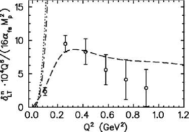
Figure 47: The $Q^{2}$ dependence of the generalized neutron polarizability $\delta_{LT}^{n}$ defined by Eq. (138). Note that $\delta_{LT}^{n}$ has been multiplied by a factor of $10^{4}Q^{6}/(16\alpha_{\text{em}}M_{p}^{2})$ in order to compensate for its rapid decrease with increasing $Q^{2}$. The open circles are the data of the JLab E 94-010 Collaboration Amarian et al. (2004a). See Fig. 42 for further notation. Figure from Drechsel and Tiator (2004).

VII conclusion

In this review we have concentrated on the bulk properties of hadrons seen at low momentum transfer, such as shape, polarizability, and low-energy excitation spectrum. We have presented many new precision data implying the compositeness of the hadrons based on the interaction among the constituents, quarks and gluons, as prescribed by the QCD Lagrangian. Experiments at high momentum transfer have established this theory as the fundamental theory of the strong interactions, with previously unexpected features like asymptotic freedom and chiral symmetry. The great success of QCD at high $Q^{2}$ has become possible by the decrease of the strong coupling constant with increasing $Q^{2}$, which allows for a perturbative treatment of QCD in this region. This is definitely not possible in the $Q^{2}$ region below 1 GeV², which defines the realm of non-perturbative QCD. Therefore, QCD has not yet passed its final tests in the low-energy domain, in which new phenomena show up, as for instance the confinement of the many-body system “hadron” and the spontaneous breaking of the chiral symmetry. In fact, QCD encounters very fundamental conceptional problems at low $Q^{2}$: One has to deal with the relativistic many-body aspect, the theoretically not yet understood confinement, and the fundamental strong interaction at the same time. The simplifications of the parton model typical for the high $Q^{2}$ physics do not work in the non-perturbative region, and neither is it possible to describe the bound many-body system of the light $u$ and $d$ quarks by basically non-relativistic physics as is done for systems of heavy quarks.

This review has two punch lines. On the experimental side one has to insist on measurements with the utmost precision. As it became evident only a new generation of cw accelerators together with modern detectors and data acquisition allowed for progress after almost two decades of stagnation. However, since the most interesting observables like spin observables are still difficult to get at, the experiments have to be well chosen. They have to be “significant” for contributing to the understanding of hadrons in the framework of QCD. For this purpose a profound theoretical guidance is needed. As promising examples of such significant experiments we mention:

• A more complete and even more precise study of meson threshold production, in particular through a study of spin observables (see section V.1) and the production of strange quarks, for example by kaon electroproduction.

• Real and virtual Compton scattering in order to disentangle all the spin polarizabilties of the nucleon by double-polarization experiments (see section IV).

• A fresh approach to investigating the excitation spectrum of the nucleon, with more attention given to the resonance-“background” separation (see section V.2). Once more, such dedicated experiments require an intense study of the spin observables. Such investigations are also the basis for further progress in understanding the sum rules discussed in section VI.

• The nucleon form factors remain a challenge at both low and high $Q^{2}$ (see section III). The improvement of the data base at low $Q^{2}$ would however take a very strong effort with the existing facilities. It is in place here to regret the closure of the MIT/Bates storage ring which offered the best means to perform such experiments at low $Q^{2}$.

On the theoretical side the challenges are not smaller. In this review we have met several effective models such as constituent quark models, dynamical baryon models, and effective meson field models. All are effective in the sense that they describe the data more or less well and provide an insight into the physics. They also provide the necessary guidance for the experiments. However, these models are only “inspired” by QCD but not fundamentally based on this theory. As of today only two schemes exist that are both directly based on QCD and able to describe the low-energy region: chiral perturbation theory (ChPT) and lattice gauge theory (LGT). Ironically the first one works best for very small quark masses, whereas the second one requires large quark masses, at least with the computer power of today. The extrapolation between these two approximations is therefore still on shaky ground. However, the ongoing efforts promise decisive turns in the near future:

• The possibilities for calculating loops beyond the leading order in ChPT is improving continously, and the necessary low-energy constants get better and better constrained by experiment and, maybe, in the near future also by LGT.

• Lattice gauge theory is progressing through more effective algorithms and the growing performance of the computers. It appears that the used quark masses will soon approach sufficiently low values to make contact with ChPT by a chiral extrapolation of the numerical results from LGT. This would indeed mark an essential breakthrough in low-energy hadron physics.

As became evident in this review, the agreement between experiment and theory is not yet satisfactory in quite a few cases, which leaves major challenges in hadron physics for both sides.

We conclude that the study of hadrons at low energy and momentum transfer is a unique possibility to unravel the structure of a relativistic many-body system in the realm of QCD, one of our most fundamentally based quantum field theories, as is highlighted by the quote from Wilczek (2000): “QCD is our most perfect physical theory.”

Acknowledgement: The authors are grateful to J. Ahrens, R. Beck, M. Distler, J. Friedrich, H. W. Hammer, B. Pasquini, F. Maas, H. Merkel, U. Müller, S. Scherer, and L. Tiator for their help and many stimulating discussions. This work was supported by the Deutsche Forschungsgemeinschaft (SFB 443). We thank the following publishers for their permission to reproduce figures: Annual Reviews for the Annual Reviews of Nuclear and Particle Science, Springer and the Italian Physical Society for the European Physical Journal A and C, and Elsevier for Physics Reports and Physics Letters.

References

- Abe et al. (1998) Abe, K., et al. (E143), 1998, Phys. Rev. D58, 112003.
- Ablikim et al. (2005) Ablikim, M., et al. (BES), 2005, Phys. Lett. B630, 14.
- Acha et al. (2007) Acha, A., et al. (HAPPEX), 2007, Phys. Rev. Lett. 98, 032301.
- Ackermann et al. (1978) Ackermann, H., et al., 1978, Nucl. Phys. B137, 294.
- Ahrens et al. (2000) Ahrens, J., et al. (GDH and A2), 2000, Phys. Rev. Lett. 84, 5950.
- Ahrens et al. (2001) Ahrens, J., et al. (GDH), 2001, Phys. Rev. Lett. 87, 022003.
- Ahrens et al. (2002) Ahrens, J., et al. (GDH), 2002, Phys. Rev. Lett. 88, 232002.
- Ahrens et al. (2003a) Ahrens, J., et al. (GDH and A2), 2003a, Eur. Phys. J. A17, 241.
- Ahrens et al. (2003b) Ahrens, J., et al. (GDH and A2), 2003b, Phys. Lett. B551, 49.
- Ahrens et al. (2004) Ahrens, J., et al. (GDH and A2), 2004, Eur. Phys. J. A21, 323.
- Ahrens et al. (2005) Ahrens, J., et al., 2005, Eur. Phys. J. A23, 113.
- Ahrens et al. (2006) Ahrens, J., et al., 2006, Phys. Rev. Lett. 97, 202303.
- Aid et al. (1995) Aid, S., et al. (H1), 1995, Z. Phys. C69, 27.
- Aiello et al. (1998) Aiello, M., M. M. Giannini, and E. Santopinto, 1998, J. Phys. G24, 753.
- Airapetian et al. (2003) Airapetian, A., et al. (HERMES), 2003, Eur. Phys. J. C26, 527.
- Alexandrou (2007) Alexandrou, C., 2007, AIP Conf. Proc. 904, 49.
- Alexandrou et al. (2006) Alexandrou, C., G. Koutsou, J. W. Negele, and A. Tsapalis, 2006, Phys. Rev. D74, 034508.
- Alexandrou et al. (2005) Alexandrou, C., et al., 2005, Phys. Rev. Lett. 94, 021601.
- Alkofer et al. (2005) Alkofer, R., A. Holl, M. Kloker, A. Krassnigg, and C. D. Roberts, 2005, Few Body Syst. 37, 1.
- Altarelli et al. (1972) Altarelli, G., N. Cabibbo, and L. Maiani, 1972, Phys. Lett. B40, 415.
- Altarelli et al. (1994) Altarelli, G., B. Lampe, P. Nason, and G. Ridolfi, 1994, Phys. Lett. B334, 187.
- Amarian et al. (2002) Amarian, M., et al., 2002, Phys. Rev. Lett. 89, 242301.
- Amarian et al. (2004a) Amarian, M., et al. (Jefferson Lab E94010), 2004a, Phys. Rev. Lett. 93, 152301.
- Amarian et al. (2004b) Amarian, M., et al. (Jefferson Lab E94-010), 2004b, Phys. Rev. Lett. 92, 022301.
- Ambrogiani et al. (1999) Ambrogiani, M., et al. (E835), 1999, Phys. Rev. D60, 032002.
- Amendolia et al. (1984) Amendolia, S. R., et al., 1984, Phys. Lett. B138, 454.
- Amendolia et al. (1986a) Amendolia, S. R., et al., 1986a, Phys. Lett. B178, 435.
- Amendolia et al. (1986b) Amendolia, S. R., et al. (NA7), 1986b, Nucl. Phys. B277, 168.
- Anderson et al. (2007) Anderson, B., et al. (Jefferson Lab E95-001), 2007, Phys. Rev. C75, 034003.
- Andreev et al. (2007) Andreev, V. A., et al. (MuCap), 2007, Phys. Rev. Lett. 99, 032002.
- Andreotti et al. (2003) Andreotti, M., et al., 2003, Phys. Lett. B559, 20.
- Aniol et al. (2004) Aniol, K. A., et al. (HAPPEX), 2004, Phys. Rev. C69, 065501.
- Aniol et al. (2006a) Aniol, K. A., et al. (HAPPEX), 2006a, Phys. Lett. B635, 275.
- Aniol et al. (2006b) Aniol, K. A., et al. (HAPPEX), 2006b, Phys. Rev. Lett. 96, 022003.
- Anselmino et al. (1989) Anselmino, M., B. L. Ioffe, and E. Leader, 1989, Sov. J. Nucl. Phys. 49, 136.
- Anthony et al. (2000) Anthony, P. L., et al. (E155), 2000, Phys. Lett. B493, 19.
- Antonelli et al. (1994) Antonelli, A., et al., 1994, Phys. Lett. B334, 431.
- Antonelli et al. (1996) Antonelli, A., et al. (FENICE), 1996, Phys. Lett. B365, 427.
- Antonelli et al. (1998) Antonelli, A., et al., 1998, Nucl. Phys. B517, 3.
- Arends and Scherer (2007) Arends, H., and S. Scherer, 2007, H1 subproject of MAMI funding proposal to DFG, CRC 443 (2008-2010) .
- Arenhövel et al. (2004) Arenhövel, H., A. Fix, and M. Schwamb, 2004, Phys. Rev. Lett. 93, 202301.
- Armstrong et al. (1999) Armstrong, C. S., et al. (Jefferson Lab E94014), 1999, Phys. Rev. D60, 052004.
- Armstrong et al. (2005) Armstrong, D. S., et al. (G0), 2005, Phys. Rev. Lett. 95, 092001.
- Armstrong et al. (1972) Armstrong, T. A., et al., 1972, Phys. Rev. D5, 1640.
- Armstrong et al. (1993) Armstrong, T. A., et al. (E760), 1993, Phys. Rev. Lett. 70, 1212.
- Arndt et al. (2002) Arndt, R. A., W. J. Briscoe, I. I. Strakovsky, and R. L. Workman, 2002, Phys. Rev. C66, 055213.
- Arndt et al. (2006) Arndt, R. A., W. J. Briscoe, I. I. Strakovsky, and R. L. Workman, 2006, Phys. Rev. C74, 045205.
- Arndt et al. (2004) Arndt, R. A., W. J. Briscoe, I. I. Strakovsky, R. L. Workman, and M. M. Pavan, 2004, Phys. Rev. C69, 035213.
- Arnold et al. (1981) Arnold, R. G., C. E. Carlson, and F. Gross, 1981, Phys. Rev. C23, 363.
- Arrington et al. (2007a) Arrington, J., W. Melnitchouk, and J. A. Tjon, 2007a, Phys. Rev. C76, 035205.
- Arrington et al. (2007b) Arrington, J., C. D. Roberts, and J. M. Zanotti, 2007b, J. Phys. G34, S23.
- Ash et al. (1967) Ash, W. W., et al., 1967, Phys. Lett. 24B, 165.
- Ciofi degli Atti and Scopetta (1997) Ciofi degli Atti, C., and S. Scopetta, 1997, Phys. Lett. B404, 223.
- Aubert et al. (2006) Aubert, B., et al. (BABAR), 2006, Phys. Rev. D73, 012005.
- Aznauryan et al. (2005) Aznauryan, I. G., et al., 2005, Phys. Rev. C71, 015201.
- Babusci et al. (1998a) Babusci, D., G. Giordano, A. I. L’vov, G. Matone, and A. M. Nathan, 1998a, Phys. Rev. C58, 1013.
- Babusci et al. (1998b) Babusci, D., G. Giordano, and G. Matone, 1998b, Phys. Rev. C57, 291.
- Baldin (1960) Baldin, A. M., 1960, Nucl. Phys. 18, 310.
- Baldini et al. (1999) Baldini, R., et al., 1999, Eur. Phys. J. C11, 709.
- Baranov et al. (1975) Baranov, P. S., et al., 1975, Yad. Fiz. 21, 689.
- Bardin et al. (1994) Bardin, G., et al., 1994, Nucl. Phys. B411, 3.
- Bass and Brisudova (1999) Bass, S. D., and M. M. Brisudova, 1999, Eur. Phys. J. A4, 251.
- Bassompierre et al. (1977) Bassompierre, G., et al. (Mulhouse-Strasbourg-Turin), 1977, Phys. Lett. B68, 477.
- Baumann (2005) Baumann, D., 2005, Produktion an der Schwelle, Ph.D. thesis, Universität Mainz, URL http://wwwa1.kph.uni-mainz.de/A1/publications/doctor/.
- Bazarko et al. (1995) Bazarko, A. O., et al. (CCFR), 1995, Z. Phys. C65, 189.
- Beane et al. (2005) Beane, S. R., M. Malheiro, J. A. McGovern, D. R. Phillips, and U. van Kolck, 2005, Nucl. Phys. A747, 311.
- Becher and Leutwyler (1999) Becher, T., and H. Leutwyler, 1999, Eur. Phys. J. C9, 643.
- Beck and Holstein (2001) Beck, D. H., and B. R. Holstein, 2001, Int. J. Mod. Phys. E10, 1.
- Beck and McKeown (2001) Beck, D. H., and R. D. McKeown, 2001, Ann. Rev. Nucl. Part. Sci. 51, 189.
- Beck (2006) Beck, R., 2006, Eur. Phys. J. A28S1, 173.
- Beck et al. (1990) Beck, R., et al., 1990, Phys. Rev. Lett. 65, 1841.
- Beck et al. (2000) Beck, R., et al., 2000, Phys. Rev. C61, 035204.
- Behrend et al. (1991) Behrend, H. J., et al. (CELLO), 1991, Z. Phys. C49, 401.
- Belinfante (1953) Belinfante, F. J., 1953, Phys. Rev. 92(4), 997.
- Belushkin et al. (2006) Belushkin, M. A., H. W. Hammer, and U.-G. Meißner, 2006, Phys. Lett. B633, 507.
- Belushkin et al. (2007) Belushkin, M. A., H. W. Hammer, and U. G. Meißner, 2007, Phys. Rev. C75, 035202.
- Bensafa et al. (2007) Bensafa, I. K., et al. (MAMi-A1), 2007, Eur. Phys. J. A32, 69.
- Bergstrom et al. (1996) Bergstrom, J. C., et al., 1996, Phys. Rev. C53, 1052.
- Bermuth et al. (2003) Bermuth, J., et al., 2003, Phys. Lett. B564, 199.
- Bermuth et al. (1988) Bermuth, K., D. Drechsel, L. Tiator, and J. B. Seaborn, 1988, Phys. Rev. D37, 89.
- Bernabeu et al. (1974) Bernabeu, J., T. E. O. Ericson, and C. Ferro Fontan, 1974, Phys. Lett. B49, 381.
- Bernard (2007) Bernard, V., 2007, eprint arXiv:0706.0312 [hep-ph].
- Bernard et al. (2002a) Bernard, V., L. Elouadrhiri, and U. G. Meißner, 2002a, J. Phys. G28, R1.
- Bernard et al. (2002b) Bernard, V., T. R. Hemmert, and U.-G. Meißner, 2002b, Phys. Lett. B545, 105.
- Bernard et al. (2003) Bernard, V., T. R. Hemmert, and U.-G. Meißner, 2003, Phys. Rev. D67, 076008.
- Bernard et al. (1991a) Bernard, V., N. Kaiser, J. Gasser, and U.-G. Meißner, 1991a, Phys. Lett. B268, 291.
- Bernard et al. (1991b) Bernard, V., N. Kaiser, and U. G. Meißner, 1991b, Phys. Rev. Lett. 67, 1515.
- Bernard et al. (1992) Bernard, V., N. Kaiser, and U. G. Meißner, 1992, Phys. Rev. Lett. 69, 1877.
- Bernard et al. (1995) Bernard, V., N. Kaiser, and U.-G. Meißner, 1995, Int. J. Mod. Phys. E4, 193.
- Bernard et al. (1996a) Bernard, V., N. Kaiser, and U.-G. Meißner, 1996a, Phys. Lett. B378, 337.
- Bernard et al. (1996b) Bernard, V., N. Kaiser, and U.-G. Meißner, 1996b, Z. Phys. C70, 483.
- Bernard et al. (1996c) Bernard, V., N. Kaiser, and U.-G. Meißner, 1996c, Nucl. Phys. A607, 379.
- Bernard et al. (2000) Bernard, V., N. Kaiser, and U.-G. Meißner, 2000, Phys. Rev. C62, 028201.
- Bernard et al. (1994) Bernard, V., N. Kaiser, U.-G. Meißner, and A. Schmidt, 1994, Z. Phys. A348, 317.
- Bernard et al. (1993) Bernard, V., N. Kaiser, A. Schmidt, and U.-G. Meißner, 1993, Phys. Lett. B319, 269.
- Bernstein et al. (1997) Bernstein, A. M., et al., 1997, Phys. Rev. C55, 1509.
- Bianchi and Thomas (1999) Bianchi, N., and E. Thomas, 1999, Phys. Lett. B450, 439.
- Birse et al. (2001) Birse, M. C., X.-D. Ji, and J. A. McGovern, 2001, Phys. Rev. Lett. 86, 3204.
- Bisello et al. (1983) Bisello, D., et al., 1983, Nucl. Phys. B224, 379.
- Bisello et al. (1990) Bisello, D., et al. (DM2), 1990, Z. Phys. C48, 23.
- Bjorken (1966) Bjorken, J. D., 1966, Phys. Rev. 148, 1467.
- Bjorken (1970) Bjorken, J. D., 1970, Phys. Rev. D1, 1376.
- Boffi et al. (1993) Boffi, S., C. Giusti, and F. D. Pacati, 1993, Phys. Rept. 226, 1.
- Boffi et al. (1996) Boffi, S., C. Giusti, F. D. Pacati, and M. Radici, 1996, Electromagnetic Response of Atomic Nuclei (Oxford University Press), ISBN 978-0198517740.
- Boffi et al. (2002) Boffi, S., et al., 2002, Eur. Phys. J. A14, 17.
- Boinepalli et al. (2006) Boinepalli, S., D. B. Leinweber, A. G. Williams, J. M. Zanotti, and J. B. Zhang, 2006, Phys. Rev. D74, 093005.
- Bosshard et al. (1991) Bosshard, A., et al., 1991, Phys. Rev. D44, 1962.
- Bourgeois et al. (2006) Bourgeois, P., et al., 2006, Phys. Rev. Lett. 97, 212001.
- Braghieri et al. (1995) Braghieri, A., et al., 1995, Phys. Lett. B363, 46.
- Brauel et al. (1977) Brauel, P., et al., 1977, Phys. Lett. B69, 253.
- Brauel et al. (1979) Brauel, P., et al., 1979, Zeit. Phys. C3, 101.
- van den Brink et al. (1995) van den Brink, H. B., et al., 1995, Phys. Rev. Lett. 74, 3561.
- Brodsky and Primack (1969) Brodsky, S. J., and J. R. Primack, 1969, Ann. Phys. 52, 315.
- Brodsky and Schmidt (1995) Brodsky, S. J., and I. Schmidt, 1995, Phys. Lett. B351, 344.
- Brown and Rho (1979) Brown, G. E., and M. Rho, 1979, Phys. Lett. B82, 177.
- Budd et al. (2003) Budd, H., A. Bodek, and J. Arrington, 2003, eprint hep-ex/0308005.
- Burkert (2001) Burkert, V. D., 2001, Phys. Rev. D63, 097904.
- Burkhardt and Cottingham (1970) Burkhardt, H., and W. N. Cottingham, 1970, Annals Phys. 56, 453.
- Capstick and Karl (1990) Capstick, S., and G. Karl, 1990, Phys. Rev. D41, 2767.
- Capstick and Keister (1995) Capstick, S., and B. D. Keister, 1995, Phys. Rev. D51, 3598.
- Cardarelli et al. (1995) Cardarelli, F., E. Pace, G. Salme, and S. Simula, 1995, Phys. Lett. B357, 267.
- Cardarelli and Simula (2000) Cardarelli, F., and S. Simula, 2000, Phys. Rev. C62, 065201.
- Cardman (2006) Cardman, L. S., 2006, Eur. Phys. J. A28S1, 7.
- Carlson and Vanderhaeghen (2007) Carlson, C. E., and M. Vanderhaeghen, 2007, Ann. Rev. Nucl. Part. Sci. 57, 171.
- Castellano et al. (1973) Castellano, M., et al., 1973, Nuovo Cim. A14, 1.
- Chew et al. (1957) Chew, G. F., M. L. Goldberger, F. E. Low, and Y. Nambu, 1957, Phys. Rev. 106, 1345.
- Christov et al. (1995) Christov, C. V., A. Z. Gorski, K. Goeke, and P. V. Pobylitsa, 1995, Nucl. Phys. A592, 513.
- Chung and Coester (1991) Chung, P. L., and F. Coester, 1991, Phys. Rev. D44, 229.
- Crawford et al. (2007) Crawford, C. B., et al., 2007, Phys. Rev. Lett. 98, 052301.
- Cudell et al. (2000) Cudell, J. R., V. Ezhela, K. Kang, S. Lugovsky, and N. Tkachenko, 2000, Phys. Rev. D61, 034019.
- De Baenst (1970) De Baenst, P., 1970, Nucl. Phys. B24, 633.
- De Rujula et al. (1975) De Rujula, A., H. Georgi, and S. L. Glashow, 1975, Phys. Rev. D12, 147.
- De Rujula et al. (1971) De Rujula, A., J. M. Kaplan, and E. De Rafael, 1971, Nucl. Phys. B35, 365.
- De Sanctis et al. (2005a) De Sanctis, M., M. M. Giannini, E. Santopinto, and A. Vassallo, 2005a, eprint nucl-th/0506033.
- De Sanctis et al. (2005b) De Sanctis, M., M. M. Giannini, E. Santopinto, and A. Vassallo, 2005b, Nucl. Phys. A755, 294.
- Delcourt et al. (1979) Delcourt, B., et al., 1979, Phys. Lett. B86, 395.
- Denizli et al. (2007) Denizli, H., et al. (CLAS), 2007, Phys. Rev. C76, 015204.
- Derrick et al. (1994) Derrick, M., et al. (ZEUS), 1994, Z. Phys. C63, 391.
- Diakonov and Petrov (1986) Diakonov, D., and V. Y. Petrov, 1986, Nucl. Phys. B272, 457.
- Diakonov et al. (1988) Diakonov, D., V. Y. Petrov, and P. V. Pobylitsa, 1988, Nucl. Phys. B306, 809.
- Dicus and Vega (2001) Dicus, D. A., and R. Vega, 2001, Phys. Lett. B501, 44.
- Distler et al. (1998) Distler, M. O., et al., 1998, Phys. Rev. Lett. 80, 2294.
- Drechsel and Bermuth (1991) Drechsel, D., and K. Bermuth, 1991, J. Phys. G 17, 1779.
- Drechsel et al. (2000) Drechsel, D., M. Gorchtein, B. Pasquini, and M. Vanderhaeghen, 2000, Phys. Rev. C61, 015204.
- Drechsel et al. (1999) Drechsel, D., O. Hanstein, S. S. Kamalov, and L. Tiator, 1999, Nucl. Phys. A645, 145.
- Drechsel et al. (2001) Drechsel, D., S. S. Kamalov, and L. Tiator, 2001, Phys. Rev. D63, 114010.
- Drechsel et al. (2007) Drechsel, D., S. S. Kamalov, and L. Tiator, 2007, eprint arXiv:0710.0306 [nucl-th].
- Drechsel et al. (1998) Drechsel, D., G. Knöchlein, A. Y. Korchin, A. Metz, and S. Scherer, 1998, Phys. Rev. C57, 941.
- Drechsel et al. (2003) Drechsel, D., B. Pasquini, and M. Vanderhaeghen, 2003, Phys. Rept. 378, 99.
- Drechsel and Tiator (1992) Drechsel, D., and L. Tiator, 1992, J. Phys. G18, 449.
- Drechsel and Tiator (2004) Drechsel, D., and L. Tiator, 2004, Ann. Rev. Nucl. Part. Sci. 54, 69.
- Drechsel and Tiator (2007) Drechsel, D., and L. Tiator, 2007, AIP Conf. Proc. 904, 129.
- Drell and Hearn (1966) Drell, S. D., and A. C. Hearn, 1966, Phys. Rev. Lett. 16, 908.
- Dutz et al. (2003) Dutz, H., et al. (GDH), 2003, Phys. Rev. Lett. 91, 192001.
- Dutz et al. (2005) Dutz, H., et al. (GDH), 2005, Phys. Rev. Lett. 94, 162001.
- Eden et al. (1994) Eden, T., et al., 1994, Phys. Rev. C50, 1749.
- Edwards et al. (2006) Edwards, R. G., et al., 2006, PoS LAT2006, 121.
- Elsner et al. (2006) Elsner, D., et al., 2006, Eur. Phys. J. A27, 91.
- Enik et al. (1997) Enik, T. L., L. V. Mitsyna, V. G. Nikolenko, A. B. Popov, and G. S. Samosvat, 1997, Phys. Atom. Nucl. 60, 567.
- Eschrich et al. (2001) Eschrich, I., et al. (SELEX), 2001, Phys. Lett. B522, 233.
- Faessler et al. (2006) Faessler, A., T. Gutsche, V. E. Lyubovitskij, and K. Pumsa-ard, 2006, Phys. Rev. D73, 114021.
- Fatemi et al. (2003) Fatemi, R., et al. (CLAS), 2003, Phys. Rev. Lett. 91, 222002.
- Federspiel et al. (1991) Federspiel, F. J., et al., 1991, Phys. Rev. Lett. 67, 1511.
- Ferrara et al. (1992) Ferrara, S., M. Porrati, and V. L. Telegdi, 1992, Phys. Rev. D46, 3529.
- Frank et al. (1996) Frank, M. R., B. K. Jennings, and G. A. Miller, 1996, Phys. Rev. C54, 920.
- Friedrich and Walcher (2003) Friedrich, J., and T. Walcher, 2003, Eur. Phys. J. A17, 607.
- Fritzsch et al. (1973) Fritzsch, H., M. Gell-Mann, and H. Leutwyler, 1973, Phys. Lett. B47, 365.
- Fuchs et al. (1996) Fuchs, M., et al., 1996, Phys. Lett. B368, 20.
- Fuchs et al. (2003) Fuchs, T., J. Gegelia, G. Japaridze, and S. Scherer, 2003, Phys. Rev. D68, 056005.
- Gail and Hemmert (2006) Gail, T. A., and T. R. Hemmert, 2006, Eur. Phys. J. A28, 91.
- Galler et al. (2001) Galler, G., et al., 2001, Phys. Lett. B503, 245.
- Galster et al. (1971) Galster, S., et al., 1971, Nucl. Phys. B32, 221.
- Gao (2003) Gao, H.-y., 2003, Int. J. Mod. Phys. E12, 1.
- Gasser et al. (2006) Gasser, J., M. A. Ivanov, and M. E. Sainio, 2006, Nucl. Phys. B745, 84.
- Gasser and Leutwyler (1984) Gasser, J., and H. Leutwyler, 1984, Ann. Phys. 158, 142.
- Gasser and Leutwyler (1985) Gasser, J., and H. Leutwyler, 1985, Nucl. Phys. B250, 465.
- Gayou et al. (2002) Gayou, O., et al. (Jefferson Lab Hall A), 2002, Phys. Rev. Lett. 88, 092301.
- Gell-Mann and Goldberger (1954) Gell-Mann, M., and M. L. Goldberger, 1954, Phys. Rev. 96, 1433.
- Gell-Mann et al. (1954) Gell-Mann, M., M. L. Goldberger, and W. E. Thirring, 1954, Phys. Rev. 95, 1612.
- Gerasimov (1965) Gerasimov, S. B., 1965, Yad. Fiz. 2, 598.
- Gerasimov (1966) Gerasimov, S. B., 1966, Sov. J. Nucl. Phys. 2, 430.
- Geshkenbein et al. (1974) Geshkenbein, B. V., B. L. Ioffe, and M. A. Shifman, 1974, Yad. Fiz. 20, 128.
- Glazier et al. (2005) Glazier, D. I., et al., 2005, Eur. Phys. J. A24, 101.
- Göckeler et al. (2006) Göckeler, M., et al., 2006, PoS LAT2006, 120.
- Gol’danski et al. (1960) Gol’danski, V. I., et al., 1960, Sov. Phys. JEPT 11, 1223.
- Goldberg (2000) Goldberg, H., 2000, Phys. Lett. B472, 280.
- Gorringe and Fearing (2004) Gorringe, T., and H. W. Fearing, 2004, Rev. Mod. Phys. 76, 31.
- Gran et al. (2006) Gran, R., et al. (K2K), 2006, Phys. Rev. D74, 052002.
- Gronberg et al. (1998) Gronberg, J., et al. (CLEO), 1998, Phys. Rev. D57, 33.
- Gross and Wilczek (1973a) Gross, D. J., and F. Wilczek, 1973a, Phys. Rev. D8, 3633.
- Gross and Wilczek (1973b) Gross, D. J., and F. Wilczek, 1973b, Phys. Rev. Lett. 30, 1343.
- Gross and Agbakpe (2006) Gross, F., and P. Agbakpe, 2006, Phys. Rev. C73, 015203.
- Guichon et al. (1995) Guichon, P. A. M., G. Q. Liu, and A. W. Thomas, 1995, Nucl. Phys. A591, 606.
- Guichon and Vanderhaeghen (1998) Guichon, P. A. M., and M. Vanderhaeghen, 1998, Prog. Part. Nucl. Phys. 41, 125.
- Guidal et al. (1997) Guidal, M., J. M. Laget, and M. Vanderhaeghen, 1997, Nucl. Phys. A627, 645.
- Hallin et al. (1993) Hallin, E. L., et al., 1993, Phys. Rev. C48, 1497.
- Hammer (2006) Hammer, H. W., 2006, Eur. Phys. J. A28, 49.
- Hammer et al. (1996) Hammer, H. W., U.-G. Meißner, and D. Drechsel, 1996, Phys. Lett. B367, 323.
- Hammer and Ramsey-Musolf (1999) Hammer, H. W., and M. J. Ramsey-Musolf, 1999, Phys. Rev. C60, 045204.
- Hanstein et al. (1997) Hanstein, O., D. Drechsel, and L. Tiator, 1997, Phys. Lett. B399, 13.
- Heil et al. (1989) Heil, W., et al., 1989, Nucl. Phys. B327, 1.
- Helbing (2006) Helbing, K., 2006, Prog. Part. Nucl. Phys. 57, 405.
- Hemmert et al. (1998) Hemmert, T. R., B. R. Holstein, J. Kambor, and G. Knöchlein, 1998, Phys. Rev. D57, 5746.
- Hemmert et al. (2000) Hemmert, T. R., B. R. Holstein, G. Knöchlein, and D. Drechsel, 2000, Phys. Rev. D62, 014013.
- Hemmert et al. (1997a) Hemmert, T. R., B. R. Holstein, G. Knöchlein, and S. Scherer, 1997a, Phys. Rev. Lett. 79, 22.
- Hemmert et al. (1997b) Hemmert, T. R., B. R. Holstein, G. Knöchlein, and S. Scherer, 1997b, Phys. Rev. D55, 2630.
- Hildebrandt et al. (2004) Hildebrandt, R. P., H. W. Griesshammer, T. R. Hemmert, and B. Pasquini, 2004, Eur. Phys. J. A20, 293.
- Hirata et al. (2003) Hirata, M., N. Katagiri, and T. Takaki, 2003, Phys. Rev. C67, 034601.
- Hofstadter (1956) Hofstadter, R., 1956, Rev. Mod. Phys. 28, 214.
- Hofstadter (1957) Hofstadter, R., 1957, Ann. Rev. Nucl. Part. Sci. 7, 231.
- Höhler (1983) Höhler, G., 1983, Pion-Nucleon Scattering, Landoldt-Boernstein, ed. H. Schopper (Springer, Berlin) I/9b2.
- Höhler (1993) Höhler, G., 1993, PiN Newslett. 9, 1.
- Höhler and Pietarinen (1975) Höhler, G., and E. Pietarinen, 1975, Phys. Lett. B53, 471.
- Höll et al. (2005) Höll, A., et al., 2005, Nucl. Phys. A755, 298.
- Holstein and Nathan (1994) Holstein, B. R., and A. M. Nathan, 1994, Phys. Rev. D49, 6101.
- Holvoet (2001) Holvoet, H., 2001, ph.D. thesis, University of Gent.
- Holzwarth (1996) Holzwarth, G., 1996, Z. Phys. A356, 339.
- Holzwarth (2002) Holzwarth, G., 2002, eprint hep-ph/0201138.
- Holzwarth (2005) Holzwarth, G., 2005, eprint hep-ph/0511194.
- Horn et al. (2006) Horn, T., et al. (Fpi2), 2006, Phys. Rev. Lett. 97, 192001.
- Hornidge et al. (2000) Hornidge, D. L., et al., 2000, Phys. Rev. Lett. 84, 2334.
- Hyde-Wright and de Jager (2004) Hyde-Wright, C. E., and K. de Jager, 2004, Ann. Rev. Nucl. Part. Sci. 54, 217.
- Isgur and Karl (1979) Isgur, N., and G. Karl, 1979, Phys. Rev. D20, 1191.
- Isgur et al. (1982) Isgur, N., G. Karl, and R. Koniuk, 1982, Phys. Rev. D25, 2394.
- Jackson (1975) Jackson, J. D., 1975, Classical Electrodynamics, John Wiley and Sons .
- Jaffe and Mende (1992) Jaffe, R. L., and P. F. Mende, 1992, Nucl. Phys. B369, 189.
- Jankowiak (2006) Jankowiak, A., 2006, Eur. Phys. J. A28S1, 149.
- Ji (1993) Ji, X.-D., 1993, Phys. Lett. B309, 187.
- Ji et al. (2000) Ji, X.-D., C.-W. Kao, and J. Osborne, 2000, Phys. Rev. D61, 074003.
- Jones and Scadron (1973) Jones, H. F., and M. D. Scadron, 1973, Ann. Phys. 81, 1.
- Jones et al. (2000) Jones, M. K., et al. (Jefferson Lab Hall A), 2000, Phys. Rev. Lett. 84, 1398.
- Joo et al. (2004) Joo, K., et al. (CLAS), 2004, Phys. Rev. C70, 042201.
- Kaiser (2003) Kaiser, N., 2003, Phys. Rev. C68, 025202.
- Kaiser et al. (1997) Kaiser, N., T. Waas, and W. Weise, 1997, Nucl. Phys. A612, 297.
- Kamalov et al. (2001) Kamalov, S. S., G.-Y. Chen, S.-N. Yang, D. Drechsel, and L. Tiator, 2001, Phys. Lett. B522, 27.
- Kamalov and Yang (1999) Kamalov, S. S., and S. N. Yang, 1999, Phys. Rev. Lett. 83, 4494.
- Kao et al. (2004) Kao, C.-W., B. Pasquini, and M. Vanderhaeghen, 2004, Phys. Rev. D70, 114004.
- Kao and Vanderhaeghen (2002) Kao, C. W., and M. Vanderhaeghen, 2002, Phys. Rev. Lett. 89, 272002.
- Karliner (1973) Karliner, I., 1973, Phys. Rev. D7, 2717.
- Karshenboim (1998) Karshenboim, S. G., 1998, eprint hep-ph/0008137.
- Kelly et al. (2007) Kelly, J. J., et al., 2007, Phys. Rev. C75, 025201.
- Klein and Nishina (1929) Klein, O., and Y. Nishina, 1929, Z. Phys. 52, 853.
- Knöchlein et al. (1995) Knöchlein, G., D. Drechsel, and L. Tiator, 1995, Z. Phys. A352, 327.
- Koch (1985) Koch, R., 1985, Z. Phys. C29, 597.
- Koester et al. (1995) Koester, L., et al., 1995, Phys. Rev. C51, 3363.
- Kogut and Susskind (1975) Kogut, J. B., and L. Susskind, 1975, Phys. Rev. D11, 395.
- Kolb et al. (2000) Kolb, N. R., et al., 2000, Phys. Rev. Lett. 85, 1388.
- Kopecky et al. (1997) Kopecky, S., et al., 1997, Phys. Rev. C56, 2229.
- Kossert et al. (2002) Kossert, K., et al., 2002, Phys. Rev. Lett. 88, 162301.
- Kotulla (2003) Kotulla, M. (TAPS/A2), 2003, Prog. Part. Nucl. Phys. 50, 295.
- Kowalski (2006) Kowalski, S., 2006, Eur. Phys. J. A28S1, 101.
- Krusche and Schadmand (2003) Krusche, B., and S. Schadmand, 2003, Prog. Part. Nucl. Phys. 51, 399.
- Krusche et al. (1995) Krusche, B., et al., 1995, Phys. Rev. Lett. 74, 3736.
- Kubis and Meißner (2001) Kubis, B., and U.-G. Meißner, 2001, Nucl. Phys. A679, 698.
- Kunz et al. (2003) Kunz, C., et al. (MIT-Bates OOPS), 2003, Phys. Lett. B564, 21.
- Laveissiere et al. (2004) Laveissiere, G., et al. (Jefferson Lab Hall A), 2004, Phys. Rev. Lett. 93, 122001.
- Leinweber et al. (2005) Leinweber, D. B., et al., 2005, Phys. Rev. Lett. 94, 212001.
- Leinweber et al. (2006) Leinweber, D. B., et al., 2006, Phys. Rev. Lett. 97, 022001.
- Olmos de Leon et al. (2001) Olmos de Leon, V., et al., 2001, Eur. Phys. J. A10, 207.
- Leukel (2001) Leukel, R., 2001, Photoproduktion neutraler Pionen am Proton mit linear polarisierten Photonen im Bereich der -Resonanz, Ph.D. thesis, Universität Mainz, URL http://wwwa2.kph.uni-mainz.de/A2/.
- Levchuk and L’vov (2000) Levchuk, M. I., and A. I. L’vov, 2000, Nucl. Phys. A674, 449.
- Lewis et al. (2003) Lewis, R., W. Wilcox, and R. M. Woloshyn, 2003, Phys. Rev. D67, 013003.
- Li et al. (1992) Li, Z.-p., V. Burkert, and Z.-j. Li, 1992, Phys. Rev. D46, 70.
- Liesenfeld et al. (1999) Liesenfeld, A., A. W. Richter, S. Sirca, et al. (A1), 1999, Phys. Lett. B468, 20.
- Low (1954) Low, F. E., 1954, Phys. Rev. 96, 1428.
- Lu et al. (1997) Lu, D.-H., A. W. Thomas, and A. G. Williams, 1997, Phys. Rev. C55, 3108.
- Lu et al. (1998) Lu, D.-H., A. W. Thomas, and A. G. Williams, 1998, Phys. Rev. C57, 2628.
- Lundin et al. (2003) Lundin, M., et al., 2003, Phys. Rev. Lett. 90, 192501.
- L’vov (1981) L’vov, A. I., 1981, Sov. J. Nucl. Phys. 34, 597.
- L’vov and Nathan (1999) L’vov, A. I., and A. M. Nathan, 1999, Phys. Rev. C 59, 1064.
- L’vov et al. (1997) L’vov, A. I., V. A. Petrun’kin, and M. Schumacher, 1997, Phys. Rev. C55, 359.
- L’vov et al. (2001) L’vov, A. I., S. Scherer, B. Pasquini, C. Unkmeir, and D. Drechsel, 2001, Phys. Rev. C64, 015203.
- Maas (2005) Maas, F. E. (A4), 2005, Prog. Part. Nucl. Phys. 55, 320.
- Maas (2006) Maas, F. E., 2006, Eur. Phys. J. A28S1, 107.
- Maas et al. (2005) Maas, F. E., et al., 2005, Phys. Rev. Lett. 94, 082001.
- MacCormick et al. (1996) MacCormick, M., et al., 1996, Phys. Rev. C53, 41.
- MacCormick et al. (1997) MacCormick, M., et al., 1997, Phys. Rev. C55, 1033.
- MacGibbon et al. (1995) MacGibbon, B. E., et al., 1995, Phys. Rev. C52, 2097.
- Madey et al. (2003) Madey, R., et al. (E93-038), 2003, Phys. Rev. Lett. 91, 122002.
- Meißner (2007) Meißner, U.-G., 2007, AIP Conf. Proc. 904, 142.
- Mergell et al. (1996) Mergell, P., U. G. Meißner, and D. Drechsel, 1996, Nucl. Phys. A596, 367.
- Merkel et al. (2002) Merkel, H., et al., 2002, Phys. Rev. Lett. 88, 012301.
- Mertz et al. (2001) Mertz, C., et al., 2001, Phys. Rev. Lett. 86, 2963.
- Merzbacher (1970) Merzbacher, E., 1970, Quantum Mechanics, John Wiley and Sons .
- Metsch et al. (2003) Metsch, B., U. Loring, D. Merten, and H. Petry, 2003, Eur. Phys. J. A18, 189.
- Metz and Drechsel (1996) Metz, A., and D. Drechsel, 1996, Z. Phys. A356, 351.
- Metz and Drechsel (1997) Metz, A., and D. Drechsel, 1997, Z. Phys. A359, 165.
- Miller (2002) Miller, G. A., 2002, Phys. Rev. C66, 032201.
- Miller (2007) Miller, G. A., 2007, Phys. Rev. Lett. 99, 112001.
- Miller and Frank (2002) Miller, G. A., and M. R. Frank, 2002, Phys. Rev. C65, 065205.
- Milner (2006) Milner, R. G., 2006, Eur. Phys. J. A28S1, 1.
- Nacher and Oset (2002) Nacher, J. C., and E. Oset, 2002, Nucl. Phys. A697, 372.
- Nefkens et al. (1978) Nefkens, B. M. K., et al., 1978, Phys. Rev. D18, 3911.
- Nikolenko and Popov (1992) Nikolenko, G., and A. Popov, 1992, Z. Phys. A 341, 365.
- Oehme (1995) Oehme, R., 1995, eprint hep-th/9511007.
- Ostrick (2006) Ostrick, M., 2006, Eur. Phys. J. A28S1, 81.
- Park and Weigel (1992) Park, N. W., and H. Weigel, 1992, Nucl. Phys. A541, 453.
- Pascalutsa and Vanderhaeghen (2005) Pascalutsa, V., and M. Vanderhaeghen, 2005, Phys. Rev. Lett. 95, 232001.
- Pascalutsa and Vanderhaeghen (2006) Pascalutsa, V., and M. Vanderhaeghen, 2006, Phys. Rev. D73, 034003.
- Pascalutsa and Vanderhaeghen (2007) Pascalutsa, V., and M. Vanderhaeghen, 2007, eprint arXiv:0709.4583 [hep-ph].
- Pascalutsa et al. (2007) Pascalutsa, V., M. Vanderhaeghen, and S. N. Yang, 2007, Phys. Rept. 437, 125.
- Pasquini and Boffi (2007) Pasquini, B., and S. Boffi, 2007, Phys. Rev. D76, 074011.
- Pasquini et al. (2007) Pasquini, B., D. Drechsel, and M. Vanderhaeghen, 2007, Phys. Rev. C76, 015203.
- Pasquini et al. (2001a) Pasquini, B., M. Gorchtein, D. Drechsel, A. Metz, and M. Vanderhaeghen, 2001a, Eur. Phys. J. A11, 185.
- Pasquini et al. (2001b) Pasquini, B., S. Scherer, and D. Drechsel, 2001b, Phys. Rev. C63, 025205.
- Passchier et al. (1999) Passchier, I., et al., 1999, Phys. Rev. Lett. 82, 4988.
- Pavan et al. (2002) Pavan, M. M., I. I. Strakovsky, R. L. Workman, and R. A. Arndt, 2002, PiN Newslett. 16, 110.
- Pedlar et al. (2005) Pedlar, T. K., et al. (CLEO), 2005, Phys. Rev. Lett. 95, 261803.
- Perdrisat et al. (2007) Perdrisat, C. F., V. Punjabi, and M. Vanderhaeghen, 2007, Prog. Part. Nucl. Phys. 59, 694.
- Plaster et al. (2006) Plaster, B., et al. (Jefferson Laboratory E93-038), 2006, Phys. Rev. C73, 025205.
- Politzer (1973) Politzer, H. D., 1973, Phys. Rev. Lett. 30, 1346.
- Pospischil et al. (2001) Pospischil, T., et al., 2001, Phys. Rev. Lett. 86, 2959.
- Powell (1949) Powell, J. L., 1949, Phys. Rev. 75, 32.
- Prange (1958) Prange, R. E., 1958, Phys. Rev. 110(1), 240.
- Punjabi et al. (2005) Punjabi, V., et al., 2005, Phys. Rev. C71, 055202.
- Rarita and Schwinger (1941) Rarita, W., and J. S. Schwinger, 1941, Phys. Rev. 60, 61.
- Roche et al. (2000) Roche, J., J. Friederich, D. Lhuillier, et al. (VCS), 2000, Phys. Rev. Lett. 85, 708.
- Rohe (2006) Rohe, D. (A1), 2006, Eur. Phys. J. A28S1, 29.
- Rose et al. (1990) Rose, K. W., et al., 1990, Phys. Lett. B234, 460.
- Rosenbluth (1950) Rosenbluth, M. N., 1950, Phys. Rev. 59, 615.
- Rosenfelder (2000) Rosenfelder, R., 2000, Phys. Lett. B479, 381.
- Rossi et al. (2006) Rossi, P., et al. (DANTE), 2006, Letter of Intent, LNF, INFN, Frascati, Italy eprint www.lnf.infn.it/conference/nucleon05/FF.
- Sachs (1962) Sachs, R. G., 1962, Phys. Rev. 126, 2256.
- Sainio (2002) Sainio, M. E., 2002, PiN Newslett. 16, 138.
- Sato and Lee (2001) Sato, T., and T. S. H. Lee, 2001, Phys. Rev. C63, 055201.
- Scherer (2003) Scherer, S., 2003, Adv. Nucl. Phys. 27, 277.
- Schiavilla and Sick (2001) Schiavilla, R., and I. Sick, 2001, Phys. Rev. C64, 041002.
- Schindler et al. (2007) Schindler, M. R., T. Fuchs, J. Gegelia, and S. Scherer, 2007, Phys. Rev. C75, 025202.
- Schindler et al. (2004) Schindler, M. R., J. Gegelia, and S. Scherer, 2004, Phys. Lett. B586, 258.
- Schmidt et al. (2001) Schmidt, A., et al., 2001, Phys. Rev. Lett. 87, 232501.
- Schmiedmayer et al. (1991) Schmiedmayer, J., P. Riehs, J. A. Harvey, and N. W. Hill, 1991, Phys. Rev. Lett. 66(8), 1015.
- Schumacher (2005) Schumacher, M., 2005, Prog. Part. Nucl. Phys. 55, 567.
- Schumacher (2007) Schumacher, M., 2007, Eur. Phys. J. A31, 327.
- Sick (1974) Sick, I., 1974, Nucl. Phys. A218, 509.
- Sick (2003) Sick, I., 2003, Phys. Lett. B576, 62.
- Silva et al. (2002) Silva, A., H.-C. Kim, and K. Goeke, 2002, Phys. Rev. D65, 014016.
- Simula et al. (2002) Simula, S., M. Osipenko, G. Ricco, and M. Taiuti, 2002, Phys. Rev. D65, 034017.
- Souder et al. (1990) Souder, P. A., et al., 1990, Phys. Rev. Lett. 65, 694.
- Sparveris et al. (2005) Sparveris, N. F., et al. (OOPS), 2005, Phys. Rev. Lett. 94, 022003.
- Sparveris et al. (2006) Sparveris, N. F., et al., 2006, Phys. Lett. eprint nucl-ex/0611033.
- Spayde et al. (2004) Spayde, D. T., et al. (SAMPLE), 2004, Phys. Lett. B583, 79.
- Stave et al. (2006) Stave, S., et al., 2006, Eur. Phys. J. A30, 471.
- Stern et al. (1933) Stern, O., et al., 1933, Z. Physik 85, 4 and 17.
- Tadevosyan et al. (2007) Tadevosyan, V., et al. (Jefferson Lab F(pi)), 2007, Phys. Rev. C75, 055205.
- Thoma (2005) Thoma, U., 2005, AIP Conf. Proc. 768, 197.
- Thomas (1984) Thomas, A. W., 1984, Adv. Nucl. Phys. 13, 1.
- Thomas and Weise (2001) Thomas, W. A., and W. Weise, 2001, The Structure of the Nucleon (Wiley-VCH, Berlin), ISBN 3-527-40297-7.
- Tsai et al. (1975) Tsai, W.-y., J. DeRaad, Lester L., and K. A. Milton, 1975, Phys. Rev. D11, 3537.
- Udem et al. (1997) Udem, T., A. Huber, B. Gross, J. Reichert, M. Prevedelli, M. Weitz, and T. W. Hänsch, 1997, Phys. Rev. Lett. 79(14), 2646.
- Vainshtein and Zakharov (1972) Vainshtein, A. I., and V. I. Zakharov, 1972, Nucl. Phys. B36, 589.
- Vanderhaeghen (1997) Vanderhaeghen, M., 1997, Phys. Lett. B402, 243.
- Vanderhaeghen et al. (1998) Vanderhaeghen, M., M. Guidal, and J. M. Laget, 1998, Phys. Rev. C57, 1454.
- Vento et al. (1980) Vento, V., M. Rho, E. M. Nyman, J. H. Jun, and G. E. Brown, 1980, Nucl. Phys. A345, 413.
- Vrana et al. (2000) Vrana, T. P., S. A. Dytman, and T. S. H. Lee, 2000, Phys. Rept. 328, 181.
- Walcher (2006) Walcher, T., 2006, Physik J. 5N12, 45.
- Wandzura and Wilczek (1977) Wandzura, S., and F. Wilczek, 1977, Phys. Lett. B72, 195.
- Warren et al. (2004) Warren, G., et al. (Jefferson Lab E93-026), 2004, Phys. Rev. Lett. 92, 042301.
- Watson (1954) Watson, K. M., 1954, Phys. Rev. 95, 228.
- Weinberg (1970) Weinberg, S., 1970, Lectures on Elementary Particles and Quantum Field Theory, Cambridge, MA: MIT Press .
- Weinberg (1973) Weinberg, S., 1973, Phys. Rev. Lett. 31, 494.
- Weinberg (1979) Weinberg, S., 1979, Physica A96, 327.
- Weiner and Weise (1985) Weiner, R., and W. Weise, 1985, Phys. Lett. B159, 85.
- Weis et al. (2007) Weis, M., et al. (A1 Collaboration), 2007, eprint arXiv:0705.3816 [nucl-ex], URL http://arxiv.org/abs/0705.3816.
- Weller (2007) Weller, H., 2007, private communication; to appear in Proceedings of the 5th International Workshop on Chiral Dynamics, Theory and Experiment (Chiral Dynamics 2006) (World Scientific publication, Singapore, 2007, to be published .
- Weller (2003) Weller, H. R., 2003, proc. of GDH 2002, eds. M. Anghinolfi et al., World Scientific, Singapore.
- Wells et al. (2001) Wells, S. P., et al. (SAMPLE), 2001, Phys. Rev. C63, 064001.
- Wess and Zumino (1971) Wess, J., and B. Zumino, 1971, Phys. Lett. B37, 95.
- Wilczek (2000) Wilczek, F., 2000, Nucl. Phys. A663, 3.
- Wilson (1974) Wilson, K. G., 1974, Phys. Rev. D10, 2445.
- Wissmann et al. (1999) Wissmann, F., et al., 1999, Nucl. Phys. A 660, 232.
- Witten (1983) Witten, E., 1983, Nucl. Phys. B223, 422.
- Yao et al. (2006) Yao, W. M., et al. (Particle Data Group), 2006, J. Phys. G33, 1, URL http://pdg.lbl.gov.
- Zieger et al. (1992) Zieger, A., et al., 1992, Phys. Lett. B278, 34.
- Ziskin (2005) Ziskin, V., 2005, Massachusetts Institute of Technology URL http://blast.lns.mit.edu/PUBLIC_RESULTS/THESES/Ziskin.pdf.