Spots, plages, and flares on $\lambda$ Andromedae and II Pegasi

Abstract

Aims. We present the results of a contemporaneous photometric and spectroscopic monitoring of two RS CVn binaries, namely $λ$~And and II~Peg. The aim of this work is to investigate the behavior of surface inhomogeneities in the atmospheres of the active components of these systems which have nearly the same temperature but different gravity.

Methods. The light curves and the modulation of the surface temperature, as recovered from line-depth ratios (LDRs), are used to map the photospheric spots, while the H$\alpha$ emission has been used as an indicator of chromospheric inhomogeneities.

Results. The spot temperatures and sizes were derived from a spot model applied to the contemporaneous light and temperature curves. We find larger and cooler spots on II Peg ($T_{\rm sp}\simeq 3600$ K) compared to $\lambda$ And ($T_{\rm sp}\simeq 3900$ K); this could be the result of both the different gravity and the higher activity level of the former. Moreover, we find a clear anti-correlation between the H$\alpha$ emission and the photospheric diagnostics (temperature and light curves). We have also detected a modulation of the intensity of the He i D₃ line with the star rotation, suggesting the presence of surface features also in the upper chromosphere of these stars. A rough reconstruction of the 3D structure of their atmospheres has been also performed by applying a spot/plage model to the light and temperature curves and to the H$\alpha$ flux modulation. In addition, a strong flare affecting the H$\alpha$, the He i D₃, and the cores of Na i D_1,2 lines has been observed on II Peg.

Conclusions. The spot/plage configuration has been reconstructed in the visible component of $\lambda$ And and II Peg which have nearly the same temperature but very different gravity and rotation periods. A close spatial association of photospheric and chromospheric active regions, at the time of our observations, has been found in both stars. Larger and cooler spots have been found on II Peg, the system with the active component of higher gravity and higher activity level. The area ratio of plages to spots seems to decrease when the spots get bigger. Moreover, with the present and literature data, a correlation between the temperature difference $\Delta T=T_{\rm ph}-T_{\rm sp}$ and the surface gravity has been also suggested.

1 Introduction

The rotational modulation of brightness and other photospheric diagnostics in late-type stars is commonly attributed to starspots on their photospheres. The presence of chromospheric inhomogeneities similar to the solar plages is pointed out by several studies based on the H$\alpha$ and/or other diagnostics (see, e.g., Strassmeier et al. 1993a; Catalano et al. 1996, 2000; Frasca et al. 1998, 2000).

The simultaneous study of photospheric (spots) and chromospheric (plages) active regions (ARs) is important for a better understanding of the physical processes occurring during the emersion of magnetic flux tubes from below the photosphere. Indeed, the relative position and size of ARs at different atmospheric levels can provide information on the magnetic field topology. In the past ten years, rotational modulation due to surface inhomogeneities at photospheric and chromospheric level has been revealed in several RS CVn binaries, (Frasca et al. 1998; Catalano et al. 2000; Biazzo et al. 2006).

Simultaneous photometric and spectroscopic observations have frequently shown a spatial association between spots and plages in RS CVn systems (Rodonò et al. 1987; Catalano et al. 1996; Frasca et al. 1998) as well as in young mildly-active solar-type stars (Frasca et al. 2000; Biazzo et al. 2007). A close plage-spot association has been also detected in very active main-sequence single stars, like the rapidly rotating star LQ Hya (Strassmeier et al. 1993a). Also in close binary systems (e.g. TZ CrB, Frasca et al. 1997) and in extremely active stars, like the components of the contact binary VW Cep (Frasca et al. 1996), there are evidences of spot-plage associations. Moreover, for some RS CVn binary systems there is some indication of a systematic longitude lag of 30^∘–50^∘ between the plages and spots (Catalano et al. 1996, 2000).

In recent works (Catalano et al. 2002; Frasca et al. 2005, hereafter Paper I and Paper II, respectively), we presented the results of a contemporaneous spectroscopic and photometric monitoring of three active single-lined (SB1) RS CVn binaries (VY~Ari, IM~Peg, and HK~Lac), showing that it is possible to recover fairly accurate spot temperature and size values by applying a spot model to contemporaneous line-depth ratios (LDRs) variation and light curves. Subsequently we have investigated the active region topology in these stars at both chromospheric and photospheric layers (Biazzo et al. 2006, hereafter Paper III).

In the present paper, a similar analysis is applied to two other active SB1 RS CVn’s, namely $\lambda$ And and II Peg, which are stars with similar effective temperatures ($T_{\rm eff}\simeq$ 4700 and 4600 K, respectively) but with different gravities, being $\log g\simeq$ 2.5 for $\lambda$ And (Donati et al. 1995) and $\log g\simeq$ 3.2 for II Peg (Berdyugina et al. 1998b).

$\lambda$ And (HD 222107) is a bright ($V=3\aas@@fstack{m}82$) and active giant, classified as G8 IV-III. Calder (1938) was the first to discover its photometric variability, whose amplitude sometimes reaches 0$\aas@@fstack{m}$30. Six years later, Walker (1944) showed that $\lambda$ And is a SB1 with an almost circular orbit of period 20$\aas@@fstack{d}$5212. It is an atypical member of the RS CVn class, because it is largely out of synchronism, its rotational period being 53$\aas@@fstack{d}$952 (Strassmeier et al. 1993b). Indeed, in most RS CVn binaries the rotational period of both components is equal to the orbital period of the system within a few percent. Thus $\lambda$ And, whose orbit is very close to be circular, is a puzzle for the theory of tidal friction (Zahn 1977), which predicts that rotational synchronization in close binaries should precede orbit circularization. It is one of the brightest of all known chromospherically active binaries. Photoelectric light curves of $\lambda$ And (Bopp & Noah 1980; Poe & Eaton 1985) show that its photometric period is somewhat variable, probably due to differential rotation and latitude drift of the spots during magnetic cycles. In addition, there is a long-term cycle of about 11 yr in the mean brightness. Photometric long-term studies have been performed also by Henry et al. (1995). Moreover, the H$\alpha$ emission has been found to be rotationally modulated and anti-correlated with the light curve (Baliunas & Dupree 1982).

II Peg (HD 224085) has been classified as a K2-3 IV-V SB1 by Rucinski (1977) who noticed that its photometric period was quite close to 6$\aas@@fstack{p}$724183, as determined by Halliday (1952) for its essentially circular orbit. It was classified as an RS CVn system by Vogt (1981a, b) who found an amplitude of the $V$ light curve of 0$\aas@@fstack{m}$43. II Peg is among the most active RS CVn binaries and belongs to a small subset of binaries, including V711 Tau and UX Ari, in which H$\alpha$ always appears in emission (Nation & Ramsey 1981). The first photoelectric light curves have been published by Chugainov (1976) Long-term studies (e.g., Henry et al. 1995; Rodonò et al. 2000) have shown dramatic changes of the photometric wave, from almost sinusoidal, to irregular or flat. Moreover, Donati et al. (1997) have clearly detected the magnetic field on this star. The so called flip-flop phenomenon (in which the dominant part of the spot activity changes the longitude every few years) has been reported in II Peg by, e.g., Berdyugina & Tuominen (1998) and Rodonò et al. (2000) and theoretically analyzed by Elstner & Korhonen (2005).

The aim of the present work is to investigate the starspot characteristics of this two active stars with the same temperature but different gravity and activity level, as well as to study the location of the excess H$\alpha$ emission and the degree of spatial superposition between surface inhomogeneities at different atmospheric levels.

2 Observations and reduction

2.1 Spectroscopy

Spectroscopic observations have been performed in 1999 and 2000 at the M. G. Fracastoro station (Serra La Nave, Mt. Etna) of Catania Astrophysical Observatory with FRESCO (Fiber-optic Reosc Echelle Spectrograph of Catania Observatory), the échelle spectrograph connected to the 91-cm telescope through an optical fiber with a 200-$\mu$m core diameter. The spectral resolution was $R=\lambda/\Delta\lambda\,\simeq\,$14 000, with a 2.6-pixel sampling.

The data reduction was performed by using the echelle task of the IRAF package following the standard steps of background subtraction, division by a flat field spectrum given by a halogen lamp, wavelength calibration using the emission lines of a Thorium–Argon lamp, and normalization to the continuum through a polynomial fit.

We have removed the telluric water vapor lines at the H$\alpha$ wavelengths using the spectra of Altair (A7 V, $v\sin i\,=\,245$ km s^-1) acquired during the observing runs. These spectra have been normalized, also inside the very broad H$\alpha$ profile, to provide valuable templates for the water vapor lines. An interactive procedure, allowing the intensity of the template lines to vary (leaving the line ratios unchanged) until a satisfactory agreement with each observed spectrum is reached, has been applied to correct the observed spectra for telluric absorption (see Frasca et al. 2000).

2.2 Photometry

The photometric observations were performed in the $B$, $V$, and $R$ Johnson filters at the Ege University Observatory. The observations were made with an un-refrigerated Hamamatsu R4457 photometer attached to the 48-cm Cassegrain telescope.

$\lambda$ And was observed from July 9 to November 2, 1999 for a total of 35 nights, using $\psi$ And and $\kappa$ And as comparison ($C$) and check ($Ck$) star, respectively. II Peg was observed from July 3 to November 21, 2000 for a total of 25 nights, using HD 224083 and BD+27$\degr$4648 as comparison and check star, respectively.

The differential magnitudes, in the sense of variable minus comparison ($V-C$), were corrected for atmospheric extinction using the seasonal average coefficients for the Ege University Observatory. The light curves were obtained by averaging individual data points taken in the same night (from 5 to 20). The standard deviation of each observed point, as measured from the differential magnitude $V-C$ and $C-Ck$, ranges from $\pm 0\aas@@fstack{m}005$ to $\pm 0\aas@@fstack{m}015$.

3 Data analysis

3.1 H$\alpha$ line analysis

The hydrogen H$\alpha$ line is one of the most useful and easily accessible indicators of chromospheric activity in the optical spectrum. Furthermore, it is very effective, both in the Sun and in active stars, for detecting chromospheric plages, due to their high contrast against the surrounding chromosphere.

II Peg is one of the few RS CVn stars which displays the H$\alpha$ line always in emission above the local continuum. For the majority of the active binaries, instead, only a filling-in of the H$\alpha$ core can be seen. In these cases, the “spectral synthesis” method, based on the comparison with synthetic spectra from radiative equilibrium models or observed spectra of non-active standard stars (reference spectra), has been successfully used (see, e.g., Herbig 1985; Barden 1985; Frasca & Catalano 1994; Montes et al. 1995). The difference between observed and reference spectrum provides, as residual, the net chromospheric H$\alpha$ emission, which can be integrated to find the total radiative losses in the line.

Since II Peg and $\lambda$ And are SB1 systems, we used only one standard star spectrum to reproduce their observed spectra. This standard star spectrum has been rotationally broadened by convolution with a rotational profile with $v\sin i=22.6$ km s^-1 for II Peg and $v\sin i=6.5$ km s^-1 for $\lambda$ And to mimic the active star in absence of chromospheric activity. Figures 1 and 3 show samples of spectra in the H$\alpha$ region of $\lambda$ And and II Peg, respectively. The residual H$\alpha$ equivalent width, $\Delta EW_{\rm H\alpha}$, has been measured by integrating all the emission profile in the difference spectrum (see the lower panel of Fig. 1).

The error, $\sigma(\Delta EW_{\rm H\alpha})$, has been evaluated by multiplying the integration range by the photometric error on each point. This latter has been estimated by the standard deviation of the observed flux values on the difference spectra in two spectral regions near the H$\alpha$ line. Although the errors $\sigma(\Delta EW_{\rm H\alpha})$ are generally a few hundredths of an Å, a very small systematic error in $\Delta EW_{\rm H\alpha}$, due to a possible contamination by chromospheric emission in the H$\alpha$ core of the reference stars, could be still present. However, this contribution can be completely neglected for very active stars, like the RS CVn systems here investigated. More information about the spectral synthesis method can be found in Frasca & Catalano (1994).

3.2 The Helium D₃ line

As a further indicator of chromospheric activity we have analyzed also the He i $\lambda$ 5876 (D₃) line, which is normally seen as an absorption feature in active stars (e.g., Huenemoerder 1986; Biazzo et al. 2006, 2007). The reference spectra adopted do not show any He i absorption nor emission, as expected for non-active stars. In this case, the spectral subtraction technique allows to emphasize the He i line, cleaning the spectrum from nearby photospheric absorption lines, and to measure its equivalent width, $EW_{\rm HeI}$. For $EW_{\rm HeI}$ we have adopted the usual convention that an absorption line has a positive $EW$.

The helium $\lambda$ 5876 line, because of its high excitation potential, is a good tracer of the regions of higher temperature and excitation in solar and stellar chromospheres. Recent models seem to indicate that the primary mechanism responsible for the formation of the He i triplet is the collisional excitation and ionization by electron impact followed by recombination cascade (Lanzafame & Byrne 1995).

In the Sun, the He i D₃ line appears as an absorption feature in plages and weak flares and in emission in strong flares (e.g., Zirin 1988). In active stars, the He i D₃ is usually observed in absorption and sometimes in emission, like during flare events in the most active RS CVn stars (Montes et al. 1997, 1999; García-Alvarez et al. 2003). This is related to the electronic temperature and density in the emitting region (e.g., Zirin 1988; Lanzafame & Byrne 1995). A contribution to the emissivity from overionisation due to coronal EUV back-radiation is expected to play a role when the transition region pressure is below 1 dyne cm^-2 (Lanzafame & Byrne 1995). This contribution is therefore relevant for moderately active stars. In any case, our analysis in independent on the detailed mechanism of formation.

3.3 Photospheric temperature from LDRs

Line-depth ratios (LDRs) can be used for detecting the temperature rotational modulation in active RS CVn stars. Such diagnostics allow to detect temperature variations as small as 10–20 K at the resolution of our spectra and with a good signal-to-noise ratio (S/N $\geq 100$). The precision of this method is improved by averaging the results from several line pairs, as discussed in Papers I and II. Typically we used from seven to fifteen line pairs, depending on the star’s $v\sin i$, in the wavelength region around 6250 Å to produce an average value of the star photospheric temperature at each phase.

We found a clear rotational modulation of the photospheric temperature recovered from LDRs for three SB1 RS CVn binaries, namely VY Ari, IM Peg, and HK Lac (Paper I). In Paper II we showed that these temperature curves are very well correlated with the contemporaneous light curves. Moreover, the simultaneous modeling of the temperature and light curves enabled us to derive temperature and size of the starspots.

In principle, rotational line-broadening must be taken into account in a technique such as the LDR. However, $v\sin i$ is usually smaller than the instrumental resolution and rotational broadening can be safely ignored. This is not the case for II Peg, whose rotational broadening ($v\sin i=22.6$ km s^-1) is larger than the resolution of our spectra. In this case we have therefore produced a LDR–$T_{\rm eff}$ calibration using rotationally broadened reference spectra. The values of temperature deduced for II Peg with these calibrations are, however, close to those found with the calibration at $v\sin i=0$ reported in Paper I.

Further information about the LDR method can be found in Papers I and II.

4 Results

4.1 $\lambda$ And

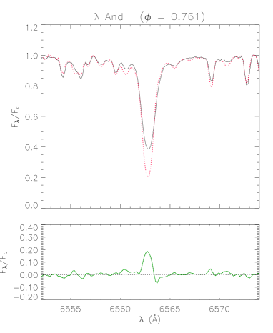
Figure 1: Top panel: Example of observed spectrum of $\lambda$ And at the rotational phase $\phi=0\aas@@fstack{p}761$ in the H$\alpha$ region (full line) together with the non-active template (dotted line). Lower panel: Difference between observed and template spectra emphasizing the core chromospheric emission.

For $\lambda$ And, nine LDRs have been used and transformed in temperature variations by means of the LDR–$T_{\rm eff}$ calibration with no rotational broadening. The rotational velocity of $\lambda$ And, namely 6.5 km s^-1 (Donati et al. 1995), is in fact lower than the FRESCO resolution of about 7 km s^-1, so that no correction for rotational broadening is needed. All the LDRs converted into temperature and combined in a single temperature curve lead to a fairly well-defined temperature variation as a function of the rotational phase and well correlated with the optical light curve (Fig. 2). Unfortunately, the very long rotation period has prevented us to obtain a complete phase coverage, but we have enough data around the maximum and minimum of the curve for performing a meaningful analysis.

The rotational phases have been derived according to the following ephemeris

$$HJD_{\phi=0}=2\,443\,829.2+53\aas@@fstack{d}952\,\times\,E\,,$$ (1)

where the initial heliocentric Julian day is that of Henry et al. (1995) and the rotational period is taken from Strassmeier et al. (1993b). The temperature maximum, with a value of 4740 K, occurs at phase $\phi\simeq 0\aas@@fstack{p}65$. The full amplitude variation of the effective temperature is $\Delta T_{\rm eff}\simeq 80$ K, corresponding to about 2% of the average temperature. The light curve displays a variation amplitude $\Delta V=0\aas@@fstack{m}$225.

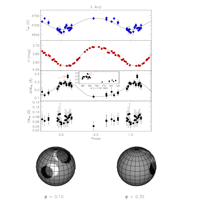
Figure 2: From top to bottom. Johnson $V$ photometry, $T_{\rm eff}$, $\Delta EW_{\rm H\alpha}$, and $EW_{\rm HeI}$ as a function of the rotational phase for $\lambda$ And. The synthetic temperature, light, and $EW_{\rm H\alpha}$ curves, calculated with our spot/plage model (see Sect. 5), are reproduced with full lines in each box. The inset displays the $\Delta EW_{\rm H\alpha}$ versus Julian Day. A schematic map of the spot and plage distributions, as seen at two different rotational phases, is also shown in the bottom.

$\mu$ Peg (G8 III), with $B-V=0\aas@@fstack{m}934$, has been used as non-active H$\alpha$ reference, because it is of the same spectral type and nearly the same color as $\lambda$ And. The H$\alpha$ line of $\lambda$ And is always in absorption but with a variable filling-in in the core (see Fig. 1 for an example). The values of the residual emission $\Delta EW_{\rm H\alpha}$ with their errors are plotted in Fig. 2 as a function of the rotational phase. Two $\Delta EW_{\rm H\alpha}$ values taken in the same nights (marked with an arrow) could be related to a mild flare event. In these hypothesis, we can only give an upper limit of two days for the flare duration, because there is no sign of H$\alpha$ enhancements either in the night before or in that following the event. It is also very difficult to estimate the flare energetics because we don’t know the flare duration and the H$\alpha$ level at the flare peak. However, we have roughly evaluated the energy released in the H$\alpha$ line during the event assuming a peak value $\Delta EW_{\rm H\alpha}=0.37$ Å (underestimate) and a flare duration of 2 days (overestimate). We have converted the net H$\alpha$ equivalent into luminosity by means of the equation:

$$L_{\rm H\alpha} = L_{6563}\Delta EW_{\rm H\alpha}=4\pi d^{2}f_{6563}\Delta EW_{\rm H\alpha}$$ (2)

$$= 4\pi d^{2}\frac{F_{6563}}{F_{5556}}10^{(-0.4V_{0}-8.451)}\Delta EW_{\rm H\alpha},$$

where $L_{6563}$ and $f_{6563}$ are the luminosity and the flux at Earth of the continuum at $\lambda=6563$ Å, $d$ is the distance and $10^{(-0.4V_{0}-8.451)}$ is the Earth flux at $\lambda=6563$ Å from a star of $V_{0}$ (de-reddened) magnitude. The continuum flux-ratio $\frac{F_{6563}}{F_{5556}}$ has been evaluated using NextGen synthetic low-resolution spectra (Hauschildt et al. 1999). We find a luminosity at peak $L_{\rm H\alpha}\raisebox{-2.15277pt}{$\>\stackrel{{\scriptstyle\textstyle<}}{{\sim}}\>$}3\times 10^{30}$ erg s^-1 and an approximate value for the total energy emitted in the H$\alpha$ line of $E_{\rm H\alpha}\approx 8\times 10^{34}$ erg.

Besides this possible flare event, a clear anti-correlation between temperature and H$\alpha$ emission is apparent with a similar shape of the curves. He i D₃ absorption has been also detected, but no clear modulation emerges from the scatter of the data.

The values of $T_{\rm eff}$, $\Delta EW_{\rm H\alpha}$, and $EW_{\rm HeI}$ for all the observed spectra are listed in Table 1.

Table 1: Temperature values and parameters of the subtracted spectra of $\lambda$ And.

HJD	Phase	$T_{\rm eff}$	$\Delta EW_{\rm H\alpha}$	$EW_{\rm HeI}$
(+2 400 000)		(K)	(Å)	(Å)
51 379.527	0.945	4683$\pm$ 7	0.22$\pm$0.03	$0.063\pm$0.018
51 379.535	0.945	4676$\pm$ 7	0.21$\pm$0.03	$0.074\pm$0.030
51 380.500	0.963	4675$\pm$ 6	0.25$\pm$0.03	$0.068\pm$0.034
51 380.512	0.964	4672$\pm$21	0.24$\pm$0.05	$0.089\pm$0.031
51 381.527	0.982	4665$\pm$ 8	0.29$\pm$0.03	$0.092\pm$0.043
51 381.539	0.983	4678$\pm$13	0.28$\pm$0.02	$0.059\pm$0.018
51 382.531	0.001	4661$\pm$ 4	0.28$\pm$0.02	$0.056\pm$0.017
51 382.539	0.001	4660$\pm$ 8	0.27$\pm$0.02	$0.049\pm$0.015
51 384.480	0.037	4665$\pm$14	0.28$\pm$0.04	$0.053\pm$0.012
51 385.527	0.056	4689$\pm$ 7	0.30$\pm$0.03	$0.066\pm$0.029
51 385.535	0.057	4687$\pm$ 6	0.30$\pm$0.02	$0.083\pm$0.027
51 386.512	0.075	4701$\pm$ 9	0.27$\pm$0.02	$0.066\pm$0.024
51 386.520	0.075	4697$\pm$10	0.27$\pm$0.03	$0.080\pm$0.025
51 387.520	0.093	4684$\pm$ 6	0.38$\pm$0.03	$0.073\pm$0.024
51 387.527	0.094	4683$\pm$ 5	0.36$\pm$0.03	$0.057\pm$0.018
51 388.523	0.112	4672$\pm$ 3	0.27$\pm$0.04	$0.078\pm$0.021
51 388.531	0.112	4686$\pm$ 5	0.26$\pm$0.03	$0.083\pm$0.021
51 389.488	0.130	4686$\pm$ 7	0.28$\pm$0.03	$0.087\pm$0.021
51 389.496	0.130	4677$\pm$ 6	0.29$\pm$0.04	$0.089\pm$0.022
51 390.488	0.148	4685$\pm$ 6	0.25$\pm$0.04	$0.072\pm$0.020
51 390.500	0.149	4700$\pm$ 9	0.24$\pm$0.06	$0.077\pm$0.019
51 407.586	0.465	4736$\pm$ 7	0.11$\pm$0.02	$0.041\pm$0.018
51 417.520	0.650	4729$\pm$11	0.15$\pm$0.03	$0.064\pm$0.023
51 417.590	0.651	4738$\pm$ 4	0.13$\pm$0.03	$0.062\pm$0.023
51 421.578	0.725	4719$\pm$ 5	0.18$\pm$0.05	$0.070\pm$0.022
51 423.520	0.761	4735$\pm$ 5	0.13$\pm$0.02	$0.063\pm$0.020
51 426.547	0.817	4716$\pm$12	0.16$\pm$0.03	$0.075\pm$0.021
51 426.555	0.817	4711$\pm$ 9	0.17$\pm$0.04	$0.067\pm$0.020

4.2 II Pegasi

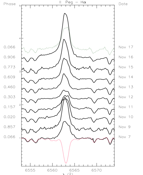
Figure 3: Time series of the H$\alpha$ profile of II Peg (full lines) together with the non-active template (dotted line). Note the very strong H$\alpha$ profile with broad wings observed during a strong flare on November 16^th followed by a nearly “normal” emission profile the night after (thin line).

Seven line-depth ratios have been used for II Peg. A few line pairs have been disregarded due to severe blending at the $v\sin i$ of II Peg. The LDR variations have been transformed into temperature variations by means of the calibration based on standard stars rotationally broadened at the same $v\sin i$ of II Peg, namely 22.6 km s^-1 (Berdyugina et al. 1998a). The rotational modulation of the temperature and $V$ magnitude is shown in the two upper boxes of Fig. 4 as a function of the phase calculated according to the following ephemeris

$$HJD_{\phi=0}=2\,443\,030.24+6\aas@@fstack{d}724333\,\times\,E\,,$$ (3)

where the rotational period and the initial epoch are taken from Berdyugina et al. (1998a) and Hall & Henry (1983), respectively. The temperature variation is about 3%, with an amplitude $\Delta T_{\rm eff}\simeq 130$ K, while the light curve amplitude is $\Delta V\simeq 0\aas@@fstack{m}63$. The two curves seem to have a slightly different shape and a small shift of the phase of minimum.

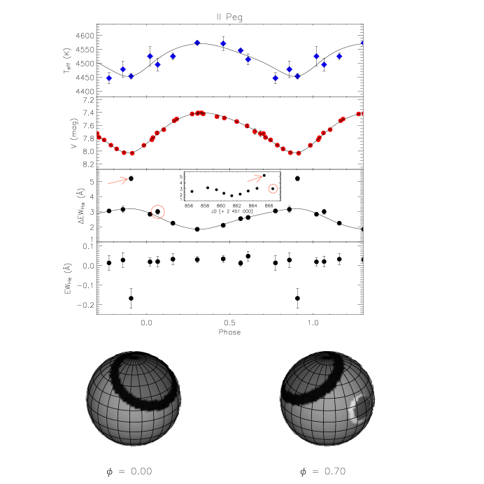
Figure 4: From top to bottom. Johnson $V$ magnitude, averaged $T_{\rm eff}$, total H$\alpha$ emission and He i D₃ equivalent width as a function of the rotational phase for II Peg. The synthetic temperature, light, and $EW_{\rm H\alpha}$ curves, calculated with our spot/plage model (see Sect. 5), are reproduced with full lines in each box. The inset displays the $\Delta EW_{\rm H\alpha}$ versus Julian Day with an arrow marking the flare peak. A schematic map of the spot and plage distributions, as seen at two different rotational phases, is also shown in the bottom.

$\delta$ Eri (K0 IV) has been used as a reference inactive star, whose spectrum has been broadened at the rotational velocity of II Peg. A sample of II Peg spectra in the H$\alpha$ region at different phases is shown in Fig. 3. The H$\alpha$ line is always in emission above the continuum level with a small core reversal from $\phi=0\aas@@fstack{p}157$ to $0\aas@@fstack{p}304$, while a pure emission with asymmetric shape is observed at other phases. A very strong and broad emission is observed at $\phi=0\aas@@fstack{p}906$. The $\Delta EW_{\rm H\alpha}$ and $EW_{\rm HeI}$ as a function of the rotational phase are plotted in Fig. 4 and listed in Table 2 together with the temperature values. In Fig. 4, a sudden increase of the H$\alpha$ equivalent width at HJD=2 451 865 ($\phi=0\aas@@fstack{p}906$), which corresponds to the onset of a flare as witnessed also by the H$\alpha$ profile, is marked with an arrow. This behavior is also present in the equivalent width of the He i line, which at that epoch was in emission (Fig. 5), unlike outside-flare spectra in which it is always in absorption. The strength of the event is also witnessed by the remarkable filling-in of the sodium D₁ and D₂ lines (Fig. 5), similarly to what found for HR 1099 by García-Alvarez et al. (2003). Since II Peg was in a quiescent phase on November 15^th, 2000, it is possible to estimate a lower limit of two days for the life of the flare, assuming that the outburst was composed by only one event. In fact, one day after the flare peak (November 17^th, HJD=2 451 866) there is still some H$\alpha$ emission excess, with respect to the average modulation curve (big circle in Fig. 4). Unfortunately, our photometric data does not include the $U$-band, sensitive to flares, and therefore no comparison with photometry can be made.

We evaluated the energy released in H$\alpha$ according to Eq. 2. Integrating the “excess luminosity” on all the duration of the flare ($\raisebox{-2.15277pt}{$\>\stackrel{{\scriptstyle\textstyle>}}{{\sim}}\>$}2$ days), the total energy emitted in the H$\alpha$ line is $E_{\rm H\alpha}^{\rm tot}\raisebox{-2.15277pt}{$\>\stackrel{{\scriptstyle\textstyle>}}{{\sim}}\>$}10^{35}$ erg. It is worth noticing that this flare has occurred near the $V$ minimum, which denotes a possible spatial association with the photospheric spots, in analogy with the most energetic solar flares, the so-called “two-ribbon” flares occurring in the biggest and more complex spotted areas. Analogously to the H$\alpha$ line, we estimated the peak luminosity for the He i line as $L_{\rm He}\approx 9\times 10^{28}$ erg s^-1 and the total emitted energy as $E_{\rm He}^{\rm tot}\leq 10^{34}$ erg. It seems that the flare had a shorter duration in the He i line, because the $EW_{\rm HeI}$ of the last spectrum is at the same level as in the quiescent phase.

Table 2: Temperature values and parameters of the subtracted spectra of II Peg.

HJD	Phase	$T_{\rm eff}$	$\Delta EW_{\rm H\alpha}$	$EW_{\rm HeI}$
(+2 400 000)		(K)	(Å)	(Å)
51 856.359	0.564	4546$\pm$ 4	2.54$\pm$0.11	$\leavevmode\nobreak\ \leavevmode\nobreak\ 0.012\pm$0.015
51 858.328	0.857	4478$\pm$29	3.15$\pm$0.21	$\leavevmode\nobreak\ \leavevmode\nobreak\ 0.028\pm$0.038
51 859.422	0.020	4525$\pm$34	2.83$\pm$0.13	$\leavevmode\nobreak\ \leavevmode\nobreak\ 0.019\pm$0.021
51 860.348	0.157	4525$\pm$11	2.24$\pm$0.12	$\leavevmode\nobreak\ \leavevmode\nobreak\ 0.032\pm$0.028
51 861.328	0.303	4573$\pm$ 7	1.84$\pm$0.11	$\leavevmode\nobreak\ \leavevmode\nobreak\ 0.030\pm$0.017
51 862.379	0.460	4570$\pm$25	2.10$\pm$0.12	$\leavevmode\nobreak\ \leavevmode\nobreak\ 0.034\pm$0.018
51 863.383	0.610	4514$\pm$20	2.62$\pm$0.12	$\leavevmode\nobreak\ \leavevmode\nobreak\ 0.047\pm$0.025
51 864.488	0.773	4446$\pm$20	3.05$\pm$0.13	$\leavevmode\nobreak\ \leavevmode\nobreak\ 0.013\pm$0.038
51 865.379	0.906	4453$\pm$10	5.19$\pm$0.15	$-0.167\pm$0.051
51 866.457	0.066	4495$\pm$23	3.00$\pm$0.16	$\leavevmode\nobreak\ \leavevmode\nobreak\ 0.020\pm$0.027

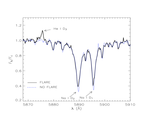
Figure 5: Two observed spectra of II Peg in the region of He i D₃ and Na i D₁,D₂ at the flare peak (full line) and in a quiescent phase (dotted line). Note the strong He i emission and the remarkable filling-in of the Na i doublet during the flare.

5 The spot/plage model

We have shown in Paper II that, with a spot model applied to contemporaneous light and temperature curves, it is possible to reconstruct the starspots distribution and to remove the degeneracy of solutions regarding spot temperature and areas. Our spot model assumes two circular active regions whose flux contrast ($F_{\rm sp}/F_{\rm ph}$) can be evaluated through the Planck spectral energy distribution (SED), the ATLAS9 (Kurucz 1993) and PHOENIX NextGen (Hauschildt et al. 1999) atmosphere models.

In Paper II we have evaluated temperature and sizes for the starspots observed on VY Ari, IM Peg, and HK Lac in the fall of 2000. We have also shown that both the atmospheric models (ATLAS9 and NextGen) provide values of the spot temperature, $T_{\rm sp}$, and area coverage in close agreement, while the black-body assumption for the SED leads to underestimate the spot temperature. This result is also in agreement with the findings of Amado et al. (1999). Since we have no long-term record of the photospheric temperature, we have assumed the maximum value obtained in our observing runs as the “unspotted” temperature for the modeling.

In order to analyze the chromospheric rotational modulations, we have extended our spot model, allowing also for bright active regions, with the aim of further investigating the degree of spot-plage correlation. Given the scatter in the data, two bright spots (plages) are fully sufficient to reproduce the observed variations.

A parameter that must be fixed in the model is the flux ratio between plages and surrounding chromosphere ($F_{\rm plage}/F_{\rm chrom}$). Values of $F_{\rm plage}/F_{\rm chrom}\,\approx\,2$, that can be deduced averaging solar plages in H$\alpha$ (e.g., Švestka 1976; Ayres et al. 1986), are too low for modeling the high amplitudes of H$\alpha$ emission curves observed for $\lambda$ And and II Peg. In fact, extremely large plages, covering a significant fraction of the stellar surface, would be required with such a low flux ratio and they could not reproduce the observed modulations. On the other hand, very high values of flux ratio ($F_{\rm plage}/F_{\rm chrom}\,\raisebox{-2.15277pt}{$\>\stackrel{{\scriptstyle\textstyle>}}{{\sim}}\>$}10$) would imply very small plages producing top-flattened modulations that are not observed. So the flux ratio was fixed to values in the range 3–8, that is also typical of the brightest parts of solar plages or of flare regions. Note that Lanzafame et al. (2000) find $F_{\rm plage}/F_{\rm chrom}\approx 3$ for HR 1099, which has $T_{\rm eff}$ and $\log g$ similar to II Peg.

The solutions essentially provide the longitude of the plages, giving only rough estimates of their latitude and size. We have searched for the best solution by varying the longitudes, latitudes and radii of the active regions. The radii are, however, strongly dependent on the assumed flux contrast $F_{\rm plage}/F_{\rm chrom}$. Thus, only the combined information between plage dimensions and flux contrast, i.e. some kind of plage “luminosity” in units of the quiet chromosphere ($L_{\rm plage}/L_{\rm quiet}$) can be deduced as a meaningful parameter. Note also that we cannot estimate the true quiet chromospheric contribution (network), since the H$\alpha$ minimum value, $\Delta EW_{\rm quiet}$, could be still affected by a homogeneous distribution of smaller plages.

5.1 $\lambda$ Andromedae

From the unspotted temperature and magnitude of $\lambda$ And, namely $T_{\rm ph}=4740$ K and the historical light maximum $V_{\rm max}=3\aas@@fstack{m}70$ (Boyd et al. 1983), and the Hipparcos parallax of 38.74$\,\pm\,$0.68 mas, the derived star radius was $R=7.51$ $R_{\odot}$. The inclination of the rotation axis with respect to the line of sight derived from this value of star radius, the $v\sin i$=6.5 km s^-1 (Donati et al. 1995), and the rotation period comes out to be $i\simeq 67\degr$. Donati et al. (1995) found the same value of the star radius and estimated an inclination $i=60\degr_{-15}^{+30}$. Since our $i$ value is the same as (Donati et al. 1995) within the errors, we adopted $i=60\degr$ for the spot modeling.

The results of the grids of solutions for the light curve and the temperature curve are displayed in Fig. 6, while the spot/plage configuration is given in Table 3 and displayed in Fig. 2 which also shows the synthetic curves superimposed to the data as full lines. In this case $F_{\rm plage}/F_{\rm chrom}$ was set to 8. A smaller contrast value would give rise to very big plages with a worse fitting of the H$\alpha$ curve.

Table 3: Spot/plage configuration for $\lambda$ And^a.

Radius	Lon.	Lat.	$T_{\rm sp}/T_{\rm ph}$	$T_{\rm sp}$	$A_{\rm rel}$
($\degr$)	($\degr$)	($\degr$)		(K)
Spots
26.5	343	57	0.815${}^{+0.064}_{-0.036}$	3861${}^{+304}_{-170}$	0.076${}^{+0.023}_{-0.014}$
17.1	64	9
Plages
22.5	360	63			0.068
19.8	48	18

^a Limb-darkening coefficients $\mu_{\rm V}$=0.797 and $\mu_{6200}$=0.68, $T_{\rm ph}=4738$ K, $\Delta EW_{\rm quiet}$=0.114 Å, and $F_{\rm plage}/F_{\rm chrom}=8$ have been used.

For $\lambda$ And, Bopp & Noah (1980) and Poe & Eaton (1985) found that the asymmetric shape of the light curve requires two spots at different longitudes and that these spots are 800–1050 K cooler than the surrounding photosphere, in close agreement with our findings. The two spots, revealed in the images of Donati et al. (1995) and covering altogether about 12% of the total stellar surface, had temperatures of 4000$\pm$300 K, while the photospheric temperature was determined to be 4800$\pm$50 K, giving a temperature difference $\Delta T\simeq 800$ K. They also calculated that the strong global magnetic fields recently detected in RS CVn systems could provide strong enough magnetic braking to explain the observed non-synchronization of $\lambda$ And’s rotation. Finally, Padmakar & Pandey (1999) find $\Delta T=800\pm 30$ K and $A_{\rm rel}=8.5\pm 0.3$ % setting $T_{\rm ph}=4800$ K and $i=60\degr$. The value of $\Delta T\simeq 850$ K derived by us is in close agreement with all these previous determinations, but O’Neal et al. (1998b) find cooler spots ($T_{\rm sp}\simeq 3650$ K) by using the TiO bands.

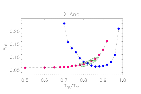
Figure 6: Grids of solutions for $\lambda$ And. The filled circles represent the values of spot temperature and area for the light-curve solutions, while the diamonds represent the solutions for the temperature curve. The hatched area, in each box, is the locus of the allowed solutions accounting for the data uncertainty.

5.2 II Pegasi

For II Peg we adopted unspotted magnitude and temperature values of $V_{\rm max}=6\aas@@fstack{m}9$ Berdyugina et al. (1998b) and $T_{\rm ph}=4573$ K (present work). From the unspotted and de-reddened $V$ magnitude and the Hipparcos parallax of 23.62 mas, a star radius of 2.76 $R_{\odot}$ is derived with the Barnes-Evans relation. From the radius, the rotational period of $6\aas@@fstack{d}724$, and the $v\sin i$ value of 22.6 km s^-1, an inclination of $60\degr_{-10}^{+30}$ has been deduced. The mass we derived from the evolutionary tracks of Girardi et al. (2000) for the primary component is 0.9 $M_{\odot}$. Berdyugina et al. (1998a) derived a mass of $0.8\pm 0.1$ $M_{\odot}$ and a radius of $3.4\pm 0.2$ $R_{\odot}$ ($\log g\simeq 3.2$) for the primary component and a mass of $0.4\pm 0.1\,M_{\odot}$ for the unseen secondary component, whose spectral type has been estimated to be M0–3V.

The result of the intersection of the grids of solutions for the light curve and the temperature curve (Fig. 7) provides a $T_{\rm sp}/T_{\rm ph}$ of 0.787, i.e a $T_{\rm sp}\simeq 3600$ K. However, the spot model with NextGen SED has been also applied and similar values to those presented in Table 4 have been found.

To reproduce the $\Delta EW_{\rm H\alpha}$ curve a relative flux $F_{\rm plage}/F_{\rm chrom}>2$ was needed. A value of $F_{\rm plage}/F_{\rm chrom}=4$ gives a satisfactory fit of the data, though, as previously outlined, this parameter cannot be constrained by the modeling of the H$\alpha$ curve. However, the analysis carried out by Busà et al. (1999) and Lanzafame et al. (2000) on HR 1099, which has $T_{\rm eff}$ and $\log g$ similar to II Peg, points to a contrast of $F_{\rm plage}/F_{\rm chrom}\approx 3$. Such analysis, based on the modeling of the Mg ii h & k and H$\alpha$ profiles, gives more constraints on the the flux contrast and the AR area.

The configuration of the active regions is represented in Fig. 4 and the active region parameters are listed in Table 4.

The first work on spot modeling for II Peg was made by Bopp & Noah (1980), who showed that, for a satisfactory modeling of their asymmetric light curve, two cool spots were sufficient. Vogt (1981a) and Huenemoerder & Ramsey (1987) made a quantitative study of the effect of spots in the TiO bands and found that a substantial fraction of the photosphere must be spotted (with a coverage of 35–40%). Then, Vogt (1981b) found that the light and color curves could be reproduced with a cool spot having an effective temperature of 3400$\pm$100 K and covering about 37% of one hemisphere on the star. In subsequent years, several other authors have produced spot models for several datasets obtained in different epochs and derived spot temperatures. Among these, the more relevant works are those of Nation & Ramsey (1981), Poe & Eaton (1985), Rodonò et al. (1986), Byrne & Marang (1987), and Boyd et al. (1987).

Donati et al. (1997), by means of the Zeeman-Doppler Imaging technique, which takes advantage of the Doppler effect in rapidly rotating stars to separate in wavelength the disk-integrated polarized profiles of magnetic lines, detected clear signatures of magnetic field with possible concentrations near the longitudes of the spots observed by Henry et al. (1995). Moreover, it was shown for this star that the changes in the light curve of II Peg are consistent with re-arrangements of the spot distribution over the stellar surface. Neff et al. (1995), from TiO molecular bands, found that cool starspots ($T_{\rm sp}$ = 3500$\pm$200 K) are always visible, with a fractional projected coverage of the visible hemisphere varying from 54% to 64% as the star rotates. O’Neal & Neff (1997) detected excess of OH absorption due to cool spots on the surface of II Peg and found a spot filling factor of 35–48%, consistent with the minimum value of 40% found by Marino et al. (1999). Hatzes (1995) revealed polar or high-latitude spots and several equatorial spots with a total coverage of about 15%. O’Neal et al. (1998a) reported the first spectroscopic evidence for the multiple spot temperature for this star. From TiO molecular band observations, they found that spot temperature varied between 3350 to 3550 K during the epoch of September 1996 to October 1996, whereas the starspot filling factor was constant (about 55%). Finally, Berdyugina et al. (1998b) found, from their surface images, that the high-latitude spots were the major contribution to the photospheric activity of II Peg. Padmakar & Pandey (1999) obtained $\Delta T=740\pm 45$ K and $A_{\rm rel}=15.7$ setting $T_{\rm ph}=4300$ K and $i=34\degr$. Recently, Gu et al. (2003), from the Doppler imaging analysis, have found for II Peg changes in spot distribution, including the position, intensity and size of the spots occurring in 1999-2001. In particular, they find in February 2000 a large high-latitude spot and a small weak low-latitude spot, i.e. the same spot configuration found in the present work for the observing season of November 2000.

Table 4: Spot/plage configuration for II Peg^a.

Radius	Lon.	Lat.	$T_{\rm sp}/T_{\rm ph}$	$T_{\rm sp}$	$A_{\rm rel}$
($\degr$)	($\degr$)	($\degr$)		(K)
Spots
47.8	320	60	0.787${}^{+0.020}_{-0.041}$	3599${}^{+91}_{-188}$ K	0.189${}^{+0.019}_{-0.018}$
16.8	202	8
Plages
35.9	322	60			0.132
18.8	206	8

^a Limb-darkening coefficients $\mu_{\rm V}$=0.836 and $\mu_{6200}$=0.74, $T_{\rm ph}=4573$ K, $\Delta EW_{\rm quiet}$=1.728 Å, and $F_{\rm plage}/F_{\rm chrom}=4$ have been used.

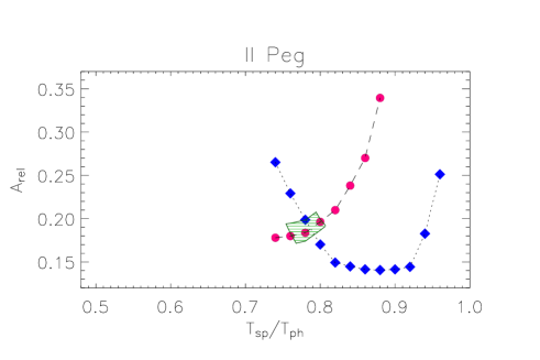
Figure 7: Grids of solutions for II Peg. The filled circles represent the values of spot temperature and area for the light-curve solutions, while the diamonds represent the solutions for the temperature curve. The hatched area, in each box, is the locus of the allowed solutions accounting for the data uncertainty.

6 Discussion

The solar paradigm can serve as a guide for the interpretation of the behaviors of stellar ARs at different atmospheric layers. In the Sun, it is found that spots are always spatially associated with faculae, although the reverse is not always true. Indeed, faculae generally form before a spot or a spot group appears and survive for some time after the disappearance of the spots. Moreover, high-latitude small faculae or plages not associated to spots are normally observed on the Sun. The ARs trace magnetic flux tube emersion, that is influenced by several effects, such as the Coriolis force, magnetic tension, and convective motions. Therefore, studies of the topology, motions, and orientations of ARs at different levels (spots, plages) can provide information about the physical processes occurring below the solar/stellar surface.

Some papers dealt with the behavior of facular to sunspot areas along the solar activity cycle (e.g., Chapman et al. 1997; Foukal 1998). In particular, Foukal (1998) found that the area ratio of faculae to spots decreases at increasing activity levels both using white-light faculae and Ca ii K chromospheric plages and explains this as a consequence of the different dependencies of plage and spot lifetimes upon their emergent magnetic flux. Thus, the sub-photospheric field properties are believed to be more important to determine this ratio, rather than photospheric field diffusion. Moreover, this shift toward dark photospheric structures for high activity levels can explain the high variation amplitudes observed in late-type stars more active than the Sun.

Some authors found that for moderately active stars the variability at optical wavelength is strongly influenced by faculae (e.g., Radick et al. 1998; Mirtorabi et al. 2003). However, the facular contribution has been proposed also for very active stars by other authors to account for the UV flux excess of active stars compared to non-active ones (Amado 2003) and to explain the blueing of the colors when the stars get fainter (e.g., Aarum Ulvås & Engvold 1999; Messina et al. 2006). The presence of faculae/plages around spots seems to be an ubiquitous phenomenon (e.g., Frasca et al. 1997, 1998; Catalano et al. 2000; Biazzo et al. 2006, 2007) and the non-detections could be due to contrast reasons.

Despite the uncertainty in deriving the radii of the plages from our H$\alpha$ variation curves, we would like to outline that the plage area is larger than that of the underlying spot for the smaller AR, while the reverse is true (the spot bigger than the plage) for the larger AR. This holds true both for $\lambda$ And and II Peg and is in line with the findings of Foukal (1998) for solar ARs.

As regards the degree of spatial correlation of spots and plages in active stars, guidelines can be represented by disk-integrated observation of the Sun. Catalano et al. (1998) report on a strong rotational modulation of the solar irradiance in the C ii $\lambda$ 1335 Å chromospheric line from UARS SOLSTICE experiment. They ascribe to chromospheric plages this modulation and show that it is highly correlated with the sunspot number. The average position of spots appears to alternately lead and lag the centroid of plages by about 30–40$\degr$, at maximum, with a possible period of 270 days. Some indication of small longitude shifts between H$\alpha$ plages and spots within this range has been found for very active stars by Catalano et al. (2000). We find that the plage longitudes in II Peg are nearly the same as those of the underlying spots. For $\lambda$ And, instead, longitude shifts of about $+17\degr$ and $-16\degr$ for the two ARs, that we consider as marginally significant due to the data scatter and phase coverage, come out from the model solution.

The investigation of possible dependencies of spot parameters like temperature and filling factor on global stellar parameters like effective temperature, gravity, activity level (rotation rate, differential rotation, etc.) is of great importance to better understand the physical mechanisms at work on the formation and evolution of ARs.

Recently, a correlation of temperature difference between the quiet photosphere and spots, $\Delta T$, with the effective temperature has been found by Berdyugina (2005). She found that, on average, $\Delta T$ is larger for the hotter stars, with values of nearly 2000 K for stars with $T_{\rm eff}\approx 6000$ K and falling down to about 200 K for M4 stars. This behavior is displayed both by giant and main-sequence stars.

It is interesting to investigate the role of the surface gravity on $\Delta T$ by selecting stars of nearly the same temperature. To further investigate this issue, we have also used the values of $\Delta T$ derived by us in Paper II for the three active giant/subgiant stars with the LDR method. In addition, we have also considered the values of $\Delta T$=1325 K and 1030 K obtained, with a typical error of $\pm 150$ K, by O’Neal et al. (2001, 2004) with the method of TiO bands for the two main sequence stars V833 Tau and EQ Vir, which have $T_{\rm eff}$ similar to the star investigated by us and $\log g\simeq 4.5$. The data of these seven active stars suggest an increasing trend of $\Delta T$ with gravity, as already proposed by O’Neal et al. (1996), that can be explained by the balance of magnetic and gas pressure in the flux tubes of active regions. However, more data are needed to further investigate this correlation.

7 Conclusion

We have presented a study of the surface inhomogeneities at both photospheric and chromospheric levels based on a contemporaneous spectroscopic and photometric monitoring of the two active RS CVn stars $\lambda$ Andromedae and II Pegasi.

From the same data set of medium-resolution optical spectra, we have obtained information about the chromospheric and photospheric surface inhomogeneities by using the H$\alpha$ emission and the photospheric temperature (from line depth ratios), respectively. Additional information coming from the light curves, together with the temperature modulations, allowed us to disentangle the effects of starspot temperature and area and deduce these parameters in a unique way. A very important indication from this work is that the the starspots of $\lambda$ And are considerably smaller and warmer than those of II Peg, notwithstanding the nearly equal photospheric temperature. At present we cannot say if this is due to the different gravity of the two active stars, being $\lambda$ And a giant with $\log g\simeq$ 2.5 and II Peg a subgiant ($\log g\simeq$ 3.2), or if it is simply the effect of the higher activity level of II Peg compared to $\lambda$ And. More active stars with different gravity and activity level must be investigated to settle this point. However, by using the values of temperature difference between photosphere and spot, $\Delta T$, for other stars from our previous works and from the literature, we find an increasing trend of $\Delta T$ versus $\log g$ that could be explained by the magnetostatic equilibrium between gas and magnetic pressure.

We have found, for all the stars observed, a tight anti-correlation between the H$\alpha$ emission and the photospheric temperature modulations, that indicates a close spatial association between photospheric spots and chromospheric plages. The largest longitude shifts between plages and spots of about $\pm 16\degr$, have been found for $\lambda$ And. Moreover, the area ratio of plages to spots seems to decrease when the spots get bigger.

Furthermore, in II Peg a strong flare affecting both the H$\alpha$ and He i lines has been observed. The energy losses in these lines have been also evaluated. A possible flare event, with a much smaller energy budget, seems to have occurred in $\lambda$ And. In the present work we have shown the great power of a coordinated photometric and spectroscopic monitoring of active stars for the study of the main properties of their active regions.