HU-EP-07/58
Imperial-TP-RR-05/2007

¹Humboldt-Universität zu Berlin, Institut für Physik,
Newtonstraße 15, D-12489 Berlin, Germany
²Jefferson Physical Laboratory, Harvard University, Cambridge, MA 02138, USA
³Theoretical Physics Group, Blackett Laboratory,
Imperial College, London, SW7 2AZ, U.K.
⁴The Institute for Mathematical Sciences,
Imperial College, London, SW7 2PG, U.K.
⁵Department of Physics, University of California,
Santa Barbara, CA 93106-9530, USA

^adrukker@physik.hu-berlin.de, ^bgiombi@physics.harvard.edu, ^cr.ricci@imperial.ac.uk, ^ddtrancan@physics.ucsb.edu

Supersymmetric Wilson loops on $S^{3}$

Nadav Drukker^1,a, Simone Giombi^2,b, Riccardo Ricci^3,4,c, Diego Trancanelli^5,d

1 Introduction

The $AdS$/CFT correspondence [2, 3, 4] relates ${\mathcal{N}}=4$ supersymmetric Yang-Mills (SYM) theory in four dimensions and string theory on $AdS_{5}\times S^{5}$. One calculates quantities at weak coupling using the gauge theory description and at strong coupling using string theory techniques, but usually the ranges of validity of the two calculations do not overlap and one cannot compare the perturbative results with those derived from string theory.

Some notable exceptions to this last statement do exist. For example the Bethe-ansatz techniques for calculating the anomalous dimensions of local operators have allowed to interpolate from weak to strong coupling. One particularly striking example are the recent results on the cusp anomalous dimension [5, 6, 7, 8, 9, 10]. An older example of such an interpolation is the circular Wilson loop operator, whose expectation value calculated from the gauge theory point of view seems to be captured by a matrix model [11, 12]. These results agree with string calculations including an infinite series of corrections in $1/N$ [13, 14, 15] as well as some proposed string calculations valid to all orders in $1/\sqrt{g_{YM}^{2}N}$ [25].

Finding such examples is a subtle art-form, and one has to progress by tiny incremental steps from trivial quantities to more complicated ones. For the spectrum of local operators the starting point were long supersymmetric operators and their small excitations [26]. Later it was understood that this problem is related to the existence of certain integrable spin-chains [27]. Bethe-ansatz techniques to calculate the spectrum to all loop order in perturbation theory were then developed and their predictions matched to the computation of quantum corrections to the semiclassical string result, see [28, 29, 30, 31, 32, 33] and references therein.

While the understanding of Wilson loops is much more fractured, the cases that are understood have again been obtained by starting with simple examples and generalizing on them. In the case of the circular loop, it can be related by a conformal transformation to the trivial straight line, where the difference between them is due to a subtle change in the global properties of the loop. Then if one considers two local deformations of the line or circle they can be analyzed again using spin-chain techniques [34]. Another family of Wilson loops that is well understood was constructed by Zarembo [35], and can also be considered as a generalization of the straight line. Like the line, these loops have trivial expectation values, and we will review them shortly.

In this paper we elaborate on the family of supersymmetric Wilson loops introduced in [36, 37] and on some techniques we can use to compute their expectation values. These loops are similar to the ones constructed by Zarembo, but their expectation values, in general, are complicated functions of $g_{YM}$ and $N$. Instead of generalizing on the straight line, they may be viewed as generalizations of the circle. As we will show, despite their complexity, in many cases there are natural guesses for what these functions are. We do not have yet the full solution for all the loops in this class, but we are optimistic that these loops reside precisely in that regime where exact calculations are within reach of current technology. It is also our hope that this construction will lead to further developments that will allow to calculate more Wilson loop operators and derive more exact results in the $AdS$/CFT correspondence.

As further motivation for the study of Wilson loops we would like to mention that there are some interesting connections between local operators and Wilson loops. One example is the relation between the cusp anomaly of a light-like Wilson line and the anomalous dimension of large spin twist-2 operators [38, 39, 40, 41, 42, 43, 44, 45, 46, 47]. Quite remarkably light-like Wilson loops with cusps have also been conjectured by Alday and Maldacena to compute gluon scattering amplitudes [48].

In the rest of the introduction we will review the construction of our Wilson loop operators and provide more details on the proof that they are supersymmetric.

In Section 2 we will go over some specific examples of families of operators with enhanced supersymmetry. The most general case in our class will preserve two supercharges, but we will show some cases with four, eight and sixteen unbroken supersymmetries. Some of the information there has already been anticipated in [36], but we go over it in much more detail and include many new results.

Section 3 contains the basic characterization of the string duals of our Wilson loops. Beyond the standard claim that they should be described by semi-classical string solutions, we find a first-order differential equation satisfied by the strings. This equation is derived by considering a novel almost complex structure on an $AdS_{4}\times S^{2}$ subspace of $AdS_{5}\times S^{5}$. Requiring that the strings are pseudo-holomorphic with respect to this almost complex structure leads to the correct boundary conditions on the strings and to preservation of the expected supersymmetry. The string world-sheets will be interpreted as calibrated surfaces and their expectation values computed in terms of the integral of the calibration form on the world-sheet. The results in this section have not been published before.

In Section 4 we discuss Wilson loops restricted to an $S^{2}$ subspace of space-time and provide some evidence, both from the gauge theory and from string theory, that those loops can be evaluated by a perturbative prescription for two-dimensional bosonic YM expanding on [37].

We complete the paper with a series of appendices. In Appendix A we collect our conventions for the superconformal algebra while in Appendix B we provide all the details for the computation of the various supergroups preserved by the loops introduced in Section 2. Appendix C is dedicated to obtaining the explicit string surfaces in $AdS_{5}\times S^{5}$ corresponding to some of the loops presented in the text. In Appendix D we review the construction of the almost complex structure for $S^{2}$ and $S^{6}$ as a warm-up for the discussion of the almost complex structure relevant to our loops presented in Section 3.1. Finally, in Appendix E we present a sample computation in the two-dimensional Yang-Mills theory for our loops restricted to an $S^{2}$.

1.1 The loops

The gauge multiplet of ${\mathcal{N}}=4$ SYM includes all fields in the theory: One gauge field, six real scalars and four complex spinor fields and it is then natural to incorporate them into the Wilson loop operator. We will consider the extra coupling of the scalars $\Phi^{I}$ (with $I=1,\cdots,6$) so the Wilson loop is [49, 50]

$$W=\frac{1}{N}\,{\rm Tr\,}\,{\mathcal{P}}\exp\oint dt(iA_{\mu}\dot{x}^{\mu}(t)+|\dot{x}|\Theta^{I}(t)\Phi^{I})\,,$$ (1.1)

where $x^{\mu}(t)$ is the path of the loop and $\Theta^{I}(t)$ are arbitrary couplings. A necessary requirement for SUSY is that the norm of $\Theta^{I}$ be one. But that alone leads only to “local” supersymmetry. If one considers the supersymmetry variation of the loop, then at every point along the loop one finds another condition for preserved supersymmetry. Only if all those conditions commute, will the loop be globally supersymmetric.

A simple way to satisfy this is if at every point one finds the same equation. This happens in the case of the straight line, where $\dot{x}^{\mu}$ is a constant vector and one takes also $\Theta^{I}$ to be a constant. This idea was generalized in a very ingenious way by Zarembo [35], who assigned for every tangent vector in $\mathbb{R}^{4}$ a unit vector in $\mathbb{R}^{6}$ by a $6\times 4$ matrix $M^{I}{}_{\mu}$ and took $|\dot{x}|\Theta^{I}=M^{I}{}_{\mu}\dot{x}^{\mu}$. That construction guarantees that if a curve is contained within a one-dimensional linear subspace of $\mathbb{R}^{4}$ it preserves half of the super-Poincaré symmetries generated by $Q$ and $\bar{Q}$ (see the notations in Appendix A). Inside a 2-plane it will preserve $1/4$, inside $\mathbb{R}^{3}$ $1/8$ of them, and for a generic curve $1/16$. In special cases the loops might also preserve some of the superconformal symmetries, generated by $S$ and $\bar{S}$. We will refer to these loops often throughout the paper and call them “$Q$-invariant loops”.

An amazing fact about those loops is that their expectation values seem to be trivial, with evidence both from perturbation theory, from $AdS$ and from a topological argument [35, 51, 52, 53, 54]. This construction can be associated to a topological twist of ${\mathcal{N}}=4$ SYM, where one identifies an $SO(4)$ subgroup of the $SO(6)$ $R$-symmetry group with the Euclidean Lorentz group. Under this twist four of the scalars become a space-time vector $\Phi_{\mu}\equiv M^{I}{}_{\mu}\Phi_{I}$ and in the Wilson loop we use a modified connection $A_{\mu}\to A_{\mu}+i\Phi_{\mu}$.

The construction we will discuss in the rest of this paper is quite similar to this, but the expectation value of the Wilson loops will in general be non-trivial. A simple way to motivate our construction is by considering a different twist, where three of the scalars are transformed into a self-dual tensor

$$\Phi_{\mu\nu}=\sigma^{i}_{\mu\nu}M^{i}{}_{I}\Phi^{I}\,,$$ (1.2)

and the Wilson loop will involve the modified connection

$$A_{\mu}\to A_{\mu}+i\Phi_{\mu\nu}x^{\nu}\,.$$ (1.3)

The important ingredient in this construction are the tensors $\sigma^{i}_{\mu\nu}$. They can be defined by the decomposition of the Lorentz generators in the anti-chiral spinor representation ($\gamma_{\mu\nu}$) into Pauli matrices $\tau_{i}$

$$\frac{1}{2}(1-\gamma^{5})\gamma_{\mu\nu}=i\sigma^{i}_{\mu\nu}\tau_{i}\,,$$ (1.4)

where we included the projector on the anti-chiral representation ($\gamma^{5}=-\gamma^{1}\gamma^{2}\gamma^{3}\gamma^{4}$). The matrix $M^{i}{}_{I}$ appearing in (1.2) is $3\times 6$ dimensional and is norm preserving, i.e. $MM^{\top}$ is the $3\times 3$ unit matrix. When we need an explicit choice of $M$ we take $M^{1}{}_{1}=M^{2}{}_{2}=M^{3}{}_{3}=1$ and all other entries zero.

These $\sigma$’s are also essentially the same as ’t Hooft’s $\eta$ symbols used in writing down the instanton solution, which is not surprising, since there the gauge field is self-dual. Finally another realization of them is in terms of the invariant one-forms on $S^{3}$

$$\sigma_{1}^{R,L} =2\left[\pm(x^{2}dx^{3}-x^{3}dx^{2})+(x^{4}dx^{1}-x^{1}dx^{4})\right]$$ (1.5)

$$\sigma_{2}^{R,L} =2\left[\pm(x^{3}dx^{1}-x^{1}dx^{3})+(x^{4}dx^{2}-x^{2}dx^{4})\right]$$

$$\sigma_{3}^{R,L} =2\left[\pm(x^{1}dx^{2}-x^{2}dx^{1})+(x^{4}dx^{3}-x^{3}dx^{4})\right],$$

where $\sigma_{i}^{R}$ are the right (or left-invariant) one-forms and $\sigma_{i}^{L}$ are the left (or right-invariant) one-forms (adhering to the conventions of [55]). We chose our construction to rely on the right-forms (and the anti-chiral spinors) so

$$\sigma_{i}^{R}=2\sigma^{i}_{\mu\nu}x^{\mu}dx^{\nu}\,.$$ (1.6)

These two realizations of $\sigma^{i}_{\mu\nu}$ will be important in our exposition. The relation to the spinor representation of the Lorentz group will be crucial for the proof of supersymmetry and the relation to the one-forms on $S^{3}$ will be important for the geometric understanding and classifications of our loops.

The Wilson loops we study in this paper can then be written in the following two ways, first in form notation and then explicitly

$$W=\frac{1}{N}{\rm Tr\,}\,{\mathcal{P}}\exp\oint\left(iA+\frac{1}{2}\sigma_{i}^{R}M^{i}{}_{I}\Phi^{I}\right)=\frac{1}{N}{\rm Tr\,}\,{\mathcal{P}}\exp\oint dx^{\mu}\left(iA_{\mu}-\sigma^{i}_{\mu\nu}x^{\nu}M^{i}{}_{I}\Phi^{I}\right).$$ (1.7)

One can of course also package the last expression in terms of the modified connection $A_{\mu}+i\Phi_{\mu\nu}x^{\nu}$.

Note that this construction involves introducing a length-scale, which can be seen by the fact that the tensor (1.2) has mass dimension one instead of two. So this construction would seem to make sense only when we fix the scale of the Wilson loop. Indeed the operator (1.7) will be supersymmetric only if we restrict the loop to be on a three dimensional sphere. This sphere may be embedded in $\mathbb{R}^{4}$, or be a fixed-time slice of $S^{3}\times\mathbb{R}$. We will always take it to be of unit radius, but it is simple to generalize to other radii by putting the radius factors where they are required by dimensionality.

1.2 Supersymmetry

We can now show that our ansatz (1.7) leads to a supersymmetric Wilson loop. The supersymmetry variation of the Wilson loop will be proportional to

$$\delta W\simeq\left(i\dot{x}^{\mu}\gamma_{\mu}-\sigma^{i}_{\mu\nu}\dot{x}^{\mu}x^{\nu}M^{i}{}_{I}\rho^{I}\gamma^{5}\right)\epsilon(x)\,,$$ (1.8)

where $\gamma_{\mu}$ and $\rho^{I}$ are respectively the gamma matrices of $SO(4)$ and $SO(6)$, the Poincaré and $R$-symmetry groups and they are taken to commute with each-other. Note that later in Section 3.1, where we discuss the strings in $AdS_{5}\times S^{5}$ that describe our loops, we will use 10-dimensional notations, where all gamma matrices anti-commute. This is achieved by the simple replacement $\rho^{I}\gamma^{5}\to\rho^{I}$. In (1.8) $\epsilon(x)$ is a conformal-Killing spinor given in $\mathbb{R}^{4}$ by two arbitrary constant 16-component Majorana-Weyl spinors as

$$\epsilon(x)=\epsilon_{0}+x^{\mu}\gamma_{\mu}\epsilon_{1}\,.$$ (1.9)

$\epsilon_{0}$ is related to the Poincaré supersymmetries while $\epsilon_{1}$ is related to the super-conformal ones.

To simplify the expressions we eliminate the matrix $M$ so there is an implicit choice of three scalars (using the index $i=1,2,3$). Then, using the fact that $x^{\mu}x^{\mu}=1$, we rearrange the variation of the loop as

$$\delta W\simeq i\dot{x}^{\mu}x^{\nu}\left(\gamma_{\mu\nu}\epsilon_{1}+i\sigma^{i}_{\mu\nu}\rho^{i}\gamma^{5}\epsilon_{0}\right)-i\dot{x}^{\mu}x^{\nu}x^{\eta}\gamma_{\eta}\left(\gamma_{\mu\nu}\epsilon_{0}+i\sigma^{i}_{\mu\nu}\rho^{i}\gamma^{5}\epsilon_{1}\right).$$ (1.10)

Requiring that this variation vanishes for arbitrary curves on $S^{3}$ leads to the two equations

$$\gamma_{\mu\nu}\epsilon_{1}+i\sigma^{i}_{\mu\nu}\rho^{i}\gamma^{5}\epsilon_{0} =0\,,$$ (1.11)

$$\gamma_{\mu\nu}\epsilon_{0}+i\sigma^{i}_{\mu\nu}\rho^{i}\gamma^{5}\epsilon_{1} =0\,.$$

These equations are not hard to solve, since $\sigma^{i}_{\mu\nu}$ are related to $\gamma_{\mu\nu}$ in the anti-chiral representation (1.4). We just need to decompose $\epsilon_{0}$ and $\epsilon_{1}$ into their chiral and anti-chiral components (labeled respectively by a $+$ and $-$ superscript) and impose

$$\tau^{i}\epsilon^{-}_{1}=\rho^{i}\epsilon^{-}_{0}\,,\qquad\epsilon_{1}^{+}=\epsilon_{0}^{+}=0\,.$$ (1.12)

To solve this set of equations we can eliminate for example $\epsilon_{0}^{-}$ from (1.12) to get

$$i\tau_{1}\epsilon_{1}^{-}=-\rho_{23}\epsilon_{1}^{-}\,,\qquad i\tau_{2}\epsilon_{1}^{-}=-\rho_{31}\epsilon_{1}^{-}\,,\qquad i\tau_{3}\epsilon_{1}^{-}=-\rho_{12}\epsilon_{1}^{-}\,.$$ (1.13)

This is a set of constraints that are consistent with each other. However it is easy to see that only two of them are independent since the commutator of any two give the remaining equation. With two independent projectors, we are thus left with two independent components of $\epsilon^{-}_{1}$, while $\epsilon^{-}_{0}$ depends on $\epsilon^{-}_{1}$. So we conclude that for a generic curve on $S^{3}$ the Wilson loop preserves $1/16$ of the original supersymmetries.

For special curves, when there are extra relations between the coordinates and their derivatives, there will be more solutions and the Wilson loops will preserve more supersymmetry. We will demonstrate this in some special cases below.

To explicitly find the two combinations of $\bar{Q}$ and $\bar{S}$ which leave the Wilson loop invariant, notice that in singling out three of the scalars the $R$-symmetry group $SU(4)$ is broken down to $SU(2)_{A}\times SU(2)_{B}$, where $SU(2)_{A}$ corresponds to rotations of $\Phi^{1},\Phi^{2},\Phi^{3}$ while $SU(2)_{B}$ rotates $\Phi^{4},\Phi^{5},\Phi^{6}$. Then we recognize that the operators appearing in (1.13) are just the generators of $SU(2)_{R}$, the anti-chiral part of the Lorentz group, and the generators of $SU(2)_{A}$, and the above equations simply state that $\epsilon^{-}_{1}$ is a singlet of the diagonal sum of $SU(2)_{R}$ and $SU(2)_{A}$, while it is a doublet of $SU(2)_{B}$. More explicitly, we can always choose a basis in which $\rho^{i}$ act as Pauli matrices on the $SU(2)_{A}$ indices, such that the equations above become

$$(\tau^{R}_{k}+\tau^{A}_{k})\epsilon^{-}_{1}=0,\qquad k=1,2,3.$$ (1.14)

If we split the $SU(4)$ index in $\epsilon^{-}_{1}$ as

$$\epsilon_{A}^{1,\,\dot{\alpha}}=\epsilon_{a}^{1,\,\dot{\alpha}\dot{a}},$$ (1.15)

where $\dot{a}$ and $a$ are respectively $SU(2)_{A}$ and $SU(2)_{B}$ indices, then the solution to (1.14) can be written as

$$\epsilon_{1\,a}=\varepsilon_{\dot{\alpha}\dot{a}}\epsilon_{a}^{1,\,\dot{\alpha}\dot{a}}.$$ (1.16)

Using any of the equations in (1.12) we can determine $\epsilon_{0}$

$$\epsilon^{-}_{0}=\tau^{R}_{3}\rho^{3}\epsilon^{-}_{1}=\tau^{R}_{3}\tau^{A}_{3}\epsilon^{-}_{1}=-\epsilon^{-}_{1},$$ (1.17)

where in the last equality we used (1.14). Our conclusion is then that the Wilson loops we introduced preserve the two supercharges

$$\bar{\mathcal{Q}}^{a}=\varepsilon^{\dot{\alpha}\dot{a}}\left(\bar{Q}^{a}_{\dot{\alpha}\dot{a}}-\bar{S}^{a}_{\dot{\alpha}\dot{a}}\right).$$ (1.18)

Besides these fermionic symmetries, our Wilson loop operators obviously preserve the bosonic symmetry $SU(2)_{B}$. Using the commutation relations of the superconformal algebra given in (A.13), it is easy to verify that the above supercharges, together with the $SU(2)_{B}$ generators $T_{ab}$, form the following superalgebra

$$\left\{\bar{\mathcal{Q}}^{a}\,,\bar{\mathcal{Q}}^{b}\right\}=2T^{ab}\,,$$ (1.19)

$$\left[T^{ab}\,,\bar{\mathcal{Q}}^{c}\right]=\varepsilon^{ca}\bar{\mathcal{Q}}^{b}-\frac{1}{2}\varepsilon^{ba}\bar{\mathcal{Q}}^{c}\,,$$

$$\left[T^{ab}\,,T^{cd}\right]=\varepsilon^{ca}T^{bd}+\varepsilon^{db}T^{ac}\,.$$

This is an $OSp(1|2)$ subalgebra of the superconformal group.

1.3 Topological twisting

As mentioned from the onset, this construction is related to a topological twisting of ${\mathcal{N}}=4$ SYM. The twisting consists of replacing $SU(2)_{R}$ with the diagonal sum of $SU(2)_{R}$ and $SU(2)_{A}$, which we can denote as $SU(2)_{R^{\prime}}$, so that the twisted Lorentz group is $SU(2)_{L}\times SU(2)_{R^{\prime}}$.

This twisting was first considered in [56] and further studied in [57] (it is their case ii)). After the twisting the supercharges decompose under $SU(2)_{L}\times SU(2)_{R^{\prime}}\times SU(2)_{B}$ as

$$(\bf{2},\bf{1},\bf{2},\bf{2})+(\bf{1},\bf{2},\bf{2},\bf{2})\rightarrow(\bf{2},\bf{2},\bf{2})+(\bf{1},\bf{3},\bf{2})+(\bf{1},\bf{1},\bf{2}).$$ (1.20)

From the above it is clear that the two supercharges ${\bar{\mathcal{Q}}}^{a}$ are in the $(\bf{1},\bf{1},\bf{2})$, and therefore they become scalars after the twisting. As usual, one would then like to regard them as BRST charges, and the Wilson loops will be observables in their cohomology.

What is new in our case is that those would-be BRST charges are not made only out of the Poincaré supersymmetries $Q$, but include also the super-conformal ones $S$. Consequently those $\bar{\mathcal{Q}}^{a}$ do not anti-commute, but rather they close on the $SU(2)_{B}$ generators (1.19). This is not a major obstacle, in the resulting topological theory one would have to consider invariance under $\bar{\mathcal{Q}}^{a}$ up to $SU(2)_{B}$ rotations, which is what is done in the framework of equivariant cohomology.

We will not pursue this direction further here.

2 Examples

We will now present some examples of Wilson loop operators with enhanced supersymmetry which are special cases of our general construction. Among several new interesting operators, we will be also able to recover some previously known examples, like the well studied $1/2$ BPS circular Wilson loop [11, 12] and the $1/4$ BPS circle of [25], and even a subclass (those living in a $\mathbb{R}^{3}$ subspace) of the $Q$-invariant Wilson loops [35] will arise in a particular “flat limit”. To illustrate the richness of the construction, we will determine in detail the explicit supersymmetries and various supergroups preserved by the different examples. The relevant notations and conventions are given in Appendix A, and some technical details of the calculations are collected in Appendix B. For a comprehensive reference on superalgebras see for example [58].

2.1 Great circle

We can first show that the well known $1/2$ BPS circular Wilson loop is included in our construction as a special example, this is simply a great circle on the $S^{3}$. In fact, it is easy to see that by our construction a maximal circle will couple to a single scalar. For example, for a circle in the $(1,2)$ plane

$$x^{\mu}=(\cos t,\sin t,0,0)$$ (2.1)

the pull-back on the loop of the left-invariant one forms (1.5) appearing in (1.7) is

$$\sigma_{1}^{R}=\sigma_{2}^{R}=0\,,\qquad\frac{1}{2}\,\sigma_{3}^{R}=dt\,,$$ (2.2)

so that the corresponding Wilson loop will couple only to $\Phi^{3}$. As a consequence, vanishing of the supersymmetry variation leads to the single constraint

$$\rho^{3}\gamma^{5}\epsilon_{0}=i\gamma_{12}\epsilon_{1}\,,$$ (2.3)

and therefore the loop preserves $16$ ($8$ chiral and $8$ anti-chiral) combinations of $Q$ and $S$ and is indeed a $1/2$ BPS operator. Using (2.3) we may write down the sixteen supercharges as

$${\mathcal{Q}}^{A}=i\gamma_{12}Q^{A}+\left(\rho^{3}S\right)^{A}\,,\qquad\bar{\mathcal{Q}}_{A}=i\gamma_{12}\bar{Q}_{A}-\left(\rho^{3}\bar{S}\right)_{A},$$ (2.4)

where $A=1,\ldots,4$ and for simplicity we have omitted Lorentz indices. Furthermore, it is not difficult to show that the $1/2$ BPS circle also preserves the bosonic group $SL(2,\mathbb{R})\times SU(2)\times SO(5)$. Here, the $SO(5)\subset SO(6)$ simply follows from the fact that the loop couples to a single scalar. The remaining symmetries $SL(2,\mathbb{R})\times SU(2)$ correspond to the subgroup of the conformal group $SO(5,1)$ which leaves the loop (2.1) invariant. It is not difficult to see that the $SU(2)$ factor is generated by

$$L_{1}\equiv\frac{1}{2}\left(P_{3}-K_{3}\right),\qquad L_{2}\equiv\frac{1}{2}\left(P_{4}-K_{4}\right),\qquad L_{3}\equiv J_{34}\,,$$ (2.5)

where $P_{\mu}$ are translations, $K_{\mu}$ are special conformal transformations and $J_{\mu\nu}$ are Lorentz generators which can be realized geometrically as

$$P_{\mu}=-i\partial_{\mu}\,,\qquad K_{\mu}=-i(x^{2}\partial_{\mu}-2x_{\mu}x^{\nu}\partial_{\nu})\,,\qquad J_{\mu\nu}=i(x_{\mu}\partial_{\nu}-x_{\nu}\partial_{\mu})\,.$$ (2.6)

Finally, the $SL(2,\mathbb{R})$ symmetry is the Möebius group in the $(1,2)$ plane generated by

$$I_{1}\equiv\frac{1}{2}\left(P_{1}+K_{1}\right),\qquad I_{2}\equiv\frac{1}{2}\left(P_{2}+K_{2}\right),\qquad I_{3}\equiv J_{12}\,.$$ (2.7)

All these bosonic symmetries, together with the above supercharges, form the supergroup $OSp(4^{\star}|4)$ (for an explicit calculation of this superalgebra, see for example [59]). Notice that this is the same supergroup preserved by the $1/2$ BPS straight line (although the explicit realization in terms of generators of $PSU(2,2|4)$ is different). This is of course expected since a straight line and a circle are related by a conformal transformation (an inversion).

A $1/2$ BPS straight line, being of the class invariant under $Q$, has trivial expectation value. On the other hand the $1/2$ BPS circle is non-trivial. In perturbation theory, using the Feynman gauge, the combined gauge-scalar propagator between two points along a loop is a non-zero constant, so that the problem of summing all non-interacting graphs (ladder diagrams) is captured by the Hermitian Gaussian matrix model [11, 12]

$$\langle W\rangle=\frac{1}{\mathcal{Z}}\int{\cal D}M\,\frac{1}{N}\mbox{Tr}\,e^{M}\,\exp\left(-\frac{2N}{\lambda}\mbox{Tr}M^{2}\right)\,,$$ (2.8)

where $M$ is an $N\times N$ Hermitian matrix and $\lambda=g^{2}_{YM}N$ is the ’t Hooft coupling. It was checked in [11] that interacting graphs do not contribute to order $\lambda^{2}$, leading to the conjecture that they may never do so. A more general argument explaining the appearance of the matrix model was given in [12], using the above mentioned fact that the circular loop is related to the straight line by a conformal transformation. This would naively imply that both Wilson loops are trivial, however the conformal transformation is singular, and the difference between the two operators is localized at the singular point, leading then to a matrix model. Notice however that this argument does not imply that the matrix model has to be Gaussian, and it is still an open problem to prove that (2.8) fully captures the VEV of the $1/2$ BPS circle. Nonetheless, this conjecture has so far passed an extensive series of non-trivial tests. For example, the large $\lambda$, $N$ limit of (2.8) can be matched against the classical action of a string world-sheet in $AdS$, and certain $1/N$ corrections were also correctly reproduced by D-branes corresponding to Wilson loops in large representations of the gauge group [13, 15, 16]. A new possible point of view on the matrix model will be discussed in Section 4, where we will argue that all loops inside a great $S^{2}\subset S^{3}$ (including in particular the $1/2$ BPS circle) seem to be related to the analogous observables in the perturbative sector of two-dimensional Yang-Mills, which can indeed be exactly solved in terms of the same Gaussian matrix model.

2.2 Hopf fibers

A new interesting system contained in our general construction can be obtained by using the description of $S^{3}$ as an Hopf fibration, namely as a $S^{1}$ bundle over $S^{2}$. Explicitly, one can write the $S^{3}$ metric as

$$ds^{2}=\frac{1}{4}\left(d\theta^{2}+\sin\theta^{2}d\phi^{2}+(d\psi+\cos\theta\,d\phi)^{2}\right),$$ (2.9)

where the range of the Euler angles is $0\leq\theta\leq\pi$, $0\leq\phi\leq 2\pi$ and $0\leq\psi\leq 4\pi$. The $S^{1}$ fiber is parameterized by $\psi$, while the base $S^{2}$ by $(\theta,\phi)$. These coordinates are related to the cartesian $x^{\mu}$ by

$$x^{1}=-\sin\frac{\theta}{2}\sin\frac{\psi-\phi}{2}\,,\qquad x^{2}=\sin\frac{\theta}{2}\cos\frac{\psi-\phi}{2}\,,$$ (2.10)

$$x^{3}=\cos\frac{\theta}{2}\sin\frac{\psi+\phi}{2}\,,\qquad\ \ x^{4}=\cos\frac{\theta}{2}\cos\frac{\psi+\phi}{2}\,.$$

Consider now a Wilson loop along a generic fiber. This loop will sit at constant $(\theta,\phi)$, while $\psi$ varies along the curve. The fibers are non-intersecting great circles of the $S^{3}$, so they will each couple to a single scalar, but the interesting fact is that all the circles in the same fibration will couple to the same scalar, in this case $\Phi^{3}$. An easy way to check this is to write the left-invariant one forms (1.5) in terms of the Euler angles

$$\sigma^{R}_{1} =-\sin\psi\,d\theta+\cos\psi\sin\theta\,d\phi\,,$$ (2.11)

$$\sigma^{R}_{2} =\cos\psi\,d\theta+\sin\psi\sin\theta\,d\phi\,,$$

$$\sigma^{R}_{3} =d\psi+\cos\theta\,d\phi\,.$$

If $\theta$ and $\phi$ are constant and $\psi(t)=2t$ (with $0\leq t\leq 2\pi$), it follows that along the loop $\sigma^{R}_{1}=\sigma^{R}_{2}=0$ and $\frac{1}{2}\sigma^{R}_{3}=dt$, as in (2.2). An equivalent way to express this fact is that a fiber only follows the vector field $\xi^{R}_{3}=\partial_{\psi}$ dual to $\sigma^{R}_{3}$. Since it is a great circle, a single loop like this is $1/2$ BPS and without loss of generality we can take it, as before, to sit in the $(1,\,2)$ plane (i.e. $\theta=\pi$).

The new feature we want to consider is when there is more than a single fiber, with the other one at $(\theta,\,\phi)$. If they are not coincident then the second one will break some of the symmetry of the single circle. As we shall show, it will project down to the anti-chiral supercharges and reduce the bosonic symmetries to $U(1)\times SO(5)$.

But before we get there, it is instructive to see how the symmetries of the single great-circle act on the other fiber. The three-sphere is mapped to itself by an $SO(4,1)$ subgroup of the conformal group generated by the rotations $J_{\mu\nu}$ and by $\frac{1}{2}(P_{\mu}+K_{\mu})$. We have seen in the previous subsection (2.7) that an $SL(2,\mathbb{R})$ subgroup of this group, obtained by restricting to $\mu,\nu=1,2$, leaves a circle in the $(1,2)$ plane invariant. So while it will not move the first fiber at $\theta=\pi$, this $SL(2,\mathbb{R})$ will act non-trivially on the other fiber.

To see this explicitly, we write the action of the generators (2.7) in terms of the Euler angles as

$$I_{1} =i\,\frac{\sin(\psi-\phi)/2}{\sin\theta/2}\left(\sin\theta\,\partial_{\theta}-\cot\frac{\psi-\phi}{2}(\partial_{\phi}-\partial_{\psi})\right)\,,$$ (2.12)

$$I_{2} =-i\,\frac{\cos(\psi-\phi)/2}{\sin\theta/2}\left(\sin\theta\,\partial_{\theta}+\tan\frac{\psi-\phi}{2}(\partial_{\phi}-\partial_{\psi})\right)\,,$$

$$I_{3} =-i(\partial_{\phi}-\partial_{\psi})\,.$$

Since all the loops are invariant under $\psi$, we can ignore all the $\partial_{\psi}$, and then the three generators act as conformal transformations on the base.

These symmetries allow us to map any point on the base (excluding $\theta=\pi$) to any other. Therefore, when considering two fibers we can take the second one at $\theta=0$, which means that it lies in the $(3,\,4)$ plane.

With this it is easy to check the supersymmetries preserved by the two fibers. The first circle imposes the constraint (2.3)

$$\rho^{3}\gamma^{5}\epsilon_{0}=i\gamma_{12}\epsilon_{1}\,,$$ (2.13)

and analogously the new one (keeping note of the orientation) will impose

$$\rho^{3}\gamma^{5}\epsilon_{0}=-i\gamma_{34}\epsilon_{1}\,,$$ (2.14)

In particular we see that $\gamma_{12}\epsilon_{1}=-\gamma_{34}\epsilon_{1}$, so $\epsilon^{1}$ is a negative eigenstate of $\gamma^{5}=-\gamma^{1}\gamma^{2}\gamma^{3}\gamma^{4}$, i.e. it is anti-chiral, so the loops preserve half the supersymmetries of a single circle, or are $1/4$ BPS. By the symmetry argument above this is true for any other fiber (or more than two fibers), which can also be verified directly, by a somewhat tedious calculation.

The corresponding supercharges preserved by the system will be essentially the same as the ones associated to the $1/2$ BPS maximal circle (2.4), except that we only select the negative chirality

$$\bar{\mathcal{Q}}_{A}=i\gamma_{12}\bar{Q}_{A}-\left(\rho^{3}\bar{S}\right)_{A}\,.$$ (2.15)

As for the bosonic symmetries, notice that of the $SL(2,\mathbb{R})\times SU(2)\times SO(5)$ symmetry of the single fiber, the only remaining symmetry on the space-time side that remains is rotations of the $\psi$ angle

$$J^{R}_{3}=\frac{1}{2}\left(J_{12}-J_{34}\right)\,.$$ (2.16)

Besides this, we have of course the $SO(5)$ symmetry following from the fact that the fibers only couple to one scalar. These bosonic symmetries form together with the fermionic generators (2.15) the supergroup $OSp(2|4)$, whose even part is indeed $SO(2)\times Sp(4)\simeq U(1)\times SO(5)$. This supergroup can be seen as the subgroup of $OSp(4^{*}|4)$ obtained by dropping the positive chirality charges in (2.4). From the point of view of the algebra, it is also natural to understand why the symmetries involving $P_{\mu}$ and $K_{\mu}$ are lost for the Hopf fibers system, as those symmetries arise from commutators of charges in (2.4) with opposite chirality.

The symmetry argument above allowed us in the case of two circles to move them relative to each-other. In perturbation theory one finds an even stronger statement, the combined gauge-scalar propagator between any two points on any two fibers is the same constant as for the single circle.

Consider for example the propagator between a point $x^{\mu}(t;\theta_{0},\phi_{0})$ on one fiber and a point $y^{\mu}(s;\theta_{1},\phi_{1})$ on a second fiber. Since both circles only couple to $\Phi^{3}$, the propagator is

$$\left\langle\Big{(}i\,\dot{x}^{\mu}A_{\mu}^{a}(x)+\Phi_{3}^{a}(x)\Big{)}\Big{(}i\,\dot{y}^{\mu}A_{\mu}^{b}(y)+\Phi_{3}^{b}(y)\Big{)}\right\rangle=\frac{g_{YM}^{2}}{4\pi^{2}}\frac{1-\dot{x}\cdot\dot{y}}{(x-y)^{2}}\,\delta^{ab}=\frac{g_{YM}^{2}}{8\pi^{2}}\,\delta^{ab}\,,$$ (2.17)

as can be checked using the explicit parametrization (2.10). Thus this system of non-intersecting circles on $S^{3}$ is reminiscent of the BPS system of parallel straight lines in flat space. In that case the lines do not interact between each other (the propagators vanish) and the observable is trivial. Here we find that the fibers do interact, however the “interaction strength” is just a constant independent of the relative distance.

Since the propagator is a constant, all ladder diagrams contributing to the correlator of several Hopf fibers can be exactly summed up using the same Gaussian matrix model describing the $1/2$ BPS circle, but with a different insertion compared to (2.8). Concretely, for a system made of $k$ fibers, the ladder diagrams contribution will be equal to

$$\langle W_{k}\rangle_{\mbox{\scriptsize ladders}}=\left\langle\left(\frac{1}{N}\mbox{Tr}\,e^{M}\right)^{k}\right\rangle_{\mbox{\scriptsize m.m.}}\,,$$ (2.18)

where the expectation value on the right hand side is taken in the Gaussian matrix model as in (2.8). Of course it would be an interesting non-trivial calculation to also evaluate the contribution (if any) of diagrams with internal vertices. At large $N$ the correlator in (2.18) will be the same as $k$ non-interacting circles and will be reproduced at strong coupling by $k$ disconnected string surfaces in $AdS$. An interesting problem, which we will not further pursue here, would be to study the possible contribution of the connected string configuration in $AdS$.

2.3 Great $S^{2}$

An infinite subfamily of operators which turns out to be very interesting is obtained by restricting the loop to lie on a great $S^{2}$ inside $S^{3}$. For concreteness, we may define this two-sphere by the condition $x^{4}=0$. From the definition of the invariant one forms one can see that on this maximal $S^{2}$ the left and right forms are no longer independent, rather

$$\sigma^{L}_{i}=-\sigma^{R}_{i}=-2\varepsilon_{ijk}x^{j}\,dx^{k}\,,$$ (2.19)

which can also be written as a cross-product. Then it is not difficult to realize that (1.10) has more solutions. Using that the left forms are related to the action of the Lorentz generators on positive chirality spinors

$$dx^{\mu}x^{\nu}\gamma_{\mu\nu}\epsilon^{+}=\frac{i}{2}\,\sigma_{i}^{L}\tau_{i}^{L}\epsilon^{+}\,,$$ (2.20)

the relation $\sigma^{L}_{i}=-\sigma^{R}_{i}$ implies that (1.10) is solved not only by the antichiral spinors satisfying

$$\tau_{i}^{R}\epsilon_{1}^{-}=\rho_{i}\epsilon_{0}^{-}\,,$$ (2.21)

but also by positive chirality spinors obeying

$$\tau_{i}^{L}\epsilon_{1}^{+}=-\rho_{i}\epsilon^{+}_{0}\,.$$ (2.22)

Combining the two chiralities, this can be also written as

$$i\gamma_{jk}\epsilon_{1}=\varepsilon_{ijk}\rho_{i}\gamma^{5}\epsilon_{0}\,.$$ (2.23)

So, contrary to the general $S^{3}$ case in (1.12), we see that now the constraints are not chiral and hence the supersymmetries are doubled. The generic Wilson loop on $S^{2}$ will therefore give a $1/8$ BPS operator. One can solve the constraints in the same way as described in Section 1.2, but we will now get two copies of the solution, one for each chirality. The four supercharges may be written explicitly as

$${\mathcal{Q}}^{a}=(i\tau_{2})^{\alpha}_{\ \dot{a}}\left(Q^{\dot{a}a}_{\alpha}+S^{\dot{a}a}_{\alpha}\right),\qquad\bar{\mathcal{Q}}^{a}=\varepsilon^{\dot{\alpha}\dot{a}}\left(\bar{Q}^{a}_{\dot{\alpha}\dot{a}}-\bar{S}^{a}_{\dot{\alpha}\dot{a}}\right).$$ (2.24)

The bosonic symmetry is also enlarged compared to the generic curve on $S^{3}$. In fact, besides invariance under the group $SU(2)_{B}\subset SO(6)$ which rotates $\Phi^{4},\Phi^{5},\Phi^{6}$, there is an extra $U(1)$ symmetry generated by

$$\frac{1}{2}\left(P_{4}-K_{4}\right)\,,$$ (2.25)

which follows from the fact that the loops satisfy $x^{4}=0$. The presence of this extra symmetry may be also understood from the algebra of the supercharges. In fact, one can see that anticommuting charges of opposite chirality precisely produces the $U(1)$ generator (2.25). In Appendix B.1 we give a detailed derivation of the algebra generated by these symmetries and prove that it is a $SU(1|2)$ superalgebra. The even part of this superalgebra is $U(1)\times SU(2)_{B}$ and the four fermionic generators transforming as $\bf{2}^{+}$ + $\bf{2}^{-}$ under the even symmetries can be obtained by defining appropriate linear combinations of the supercharges (2.24).

A generic smooth curve on $S^{2}$ exhibits a curious property, whose precise significance would be interesting to explore in more depth: The gauge coupling for that curve is given, using vector notation in $\mathbb{R}^{3}$, by $\dot{\vec{x}}$ while from (2.19) the scalar coupling is the cross-product $\vec{x}\times\dot{\vec{x}}$. If we take $|\dot{\vec{x}}|=1$, then $\vec{x}\times\dot{\vec{x}}$ is also a vector on $S^{2}$ and we can consider Wilson loops along that path in space-time. The corresponding scalar coupling will be

$$\left(\vec{x}\times\dot{\vec{x}}\right)\times\left(\vec{x}\times\ddot{\vec{x}}\right)=-\vec{x}\left(\dot{\vec{x}}\cdot\vec{x}\times\ddot{\vec{x}}\right)\propto\vec{x}\,.$$ (2.26)

The proportionality constant $\vec{x}\times\ddot{\vec{x}}$ is non-zero if the curve is nowhere a geodesic (i.e. it is never part of a great circle). We see then that for any smooth, nowhere geodesic curve on $S^{2}$ there is a dual curve with gauge and scalar coupling interchanged. In Section 3.4 we comment on the extension of this map to the dual $AdS_{5}\times S^{5}$. Only on the boundary is it a map between $AdS_{5}$ and $S^{5}$, otherwise it mixes the coordinates in a somewhat more complicated way (see (3.68) and the discussion after it).

In the following subsections we discuss some examples of special loops inside $S^{2}$ preserving some extra supersymmetries. The case of the general loops belonging to this class is presented in great detail in Section 4, where we provide evidence that they are related to Wilson loops in two-dimensional Yang-Mills theory.

2.3.1 Latitude

Taking the loop to be at the equator of the $S^{2}$ will clearly give the $1/2$ BPS circle described in Section 2.1. More generally we can take the loop to be a non-maximal circle, i.e. a latitude of the $S^{2}$. Concretely, we can parameterize the loop as

$$x^{\mu}=(\sin\theta_{0}\cos t\,,\sin\theta_{0}\sin t\,,\cos\theta_{0},\,0)\,.$$ (2.27)

Computing the scalar couplings for this curve according to (2.19)

$$\frac{1}{2}\,\sigma_{i}^{R}=\varepsilon_{ijk}x^{j}\,dx^{k}=\sin\theta_{0}(-\cos\theta_{0}\cos t\,,-\cos\theta_{0}\sin t\,,\sin\theta_{0})\,dt\,,$$ (2.28)

one can see that they also describe a latitude on the $S^{2}\subset S^{5}$ associated to $\Phi^{1}$, $\Phi^{2}$, $\Phi^{3}$, but the circle sits at $\pi/2-\theta_{0}$, see figure 1. In particular, when the loop is a maximal circle, $\theta_{0}=\pi/2$, the curve in scalar space reduces to a point (the north pole) and one falls back to the $1/2$ BPS circle described in Section 2.1.

Figure 1: Quarter-BPS Wilson loop along a latitude. In a. we show the Wilson loop along a latitude at angle $\theta_{0}$ on an $S^{2}\subset\mathbb{R}^{4}$. b. depicts the scalar couplings which follow a dual latitude on $S^{2}\subset S^{5}$. Notice that if we took b. to be the path of the loop in space, then a. would describe the associated scalar couplings. This is an explicit example of the duality between scalar and gauge field couplings discussed in the text.

This family of loops is essentially the same as the operators considered in [25]: The operator we describe here and the one in [25] are simply related by a conformal transformation (a dilatation and a translation along $x^{3}$) which moves the circle from the equator to a parallel.

As can be seen from (2.28), such an operator couples to three scalars, but it can be shown that the supersymmetry equations will give only two independent constraints. Indeed, one can see that the supersymmetry variation vanishes at every point along the loop provided that the following two conditions are satisfied

$$\begin{gathered}\cos\theta_{0}\big{(}\gamma_{12}+\rho_{12}\big{)}\epsilon_{1}=0,\\ \rho^{3}\gamma^{5}\epsilon_{0}=\big{[}i\gamma_{12}+\gamma_{3}\rho^{2}\gamma^{5}\cos\theta_{0}(\gamma_{23}+\rho_{23})\big{]}\epsilon_{1}\,.\end{gathered}$$ (2.29)

If $\cos\theta_{0}\neq 0$, one has two independent constraints and the loop preserves $1/4$ of the supersymmetries. In the special case $\cos\theta_{0}=0$ the first constraint disappears and one recovers the $1/2$ BPS maximal circle condition (2.3).

One may solve the constraints (2.29) as described in Section 1.2 by viewing $\gamma_{i}$ and $\rho_{i}$ as Pauli matrices acting on Lorentz and $SU(2)_{A}$ indices respectively. In particular, the first line in (2.29) may be written as

$$(-i\gamma_{12}+\tau_{3}^{A})\epsilon_{1}=0.$$ (2.30)

For a generic loop we had three such equations (for the anti-chiral spinor), which meant that the only solution had to be a singlet of the diagonal $SU(2)_{R}+SU(2)_{A}$ group. Here we find only one such equation for each of the chiralities, such that a $U(1)$ charge ($\tau_{3}^{\text{total}}$) has to vanish. So in addition to the singlet, this constraint allows one of the states of the triplet. Explicitly, we can write the two solutions of (2.30) as

$$\epsilon_{1,\,a}^{(1)} =\epsilon_{1,\,\dot{1}\,a}^{2}-\epsilon_{1,\,\dot{2}\,a}^{1}=(i\tau_{2})^{\dot{a}}_{\ \alpha}\,\epsilon_{1,\,\dot{a}\,a}^{\alpha}$$ (2.31)

$$\epsilon_{1,\,a}^{(2)} =\epsilon_{1,\,\dot{2}\,a}^{1}+\epsilon_{1,\,\dot{1}\,a}^{2}=(\tau_{1})^{\dot{a}}_{\ \alpha}\,\epsilon_{1,\,\dot{a}a}^{\alpha}\,,$$

and similarly for the other chirality. The $\epsilon_{0}$ spinors can be obtained by solving the second line of the constraints. For the singlet spinor $\epsilon_{1}^{(1)}$, the term proportional to $\cos\theta_{0}$ does not contribute and the solution is the same as the one for the great $S^{2}$ loops given in equation (2.24), that is

$${\mathcal{Q}}_{(1)}^{a}=(i\tau_{2})^{\alpha}_{\ \dot{a}}\left(Q^{\dot{a}a}_{\alpha}+S^{\dot{a}a}_{\alpha}\right)\,,\qquad\qquad\bar{\mathcal{Q}}_{(1)}^{a}=\varepsilon^{\dot{\alpha}\dot{a}}\left(\bar{Q}^{a}_{\dot{\alpha}\dot{a}}-\bar{S}^{a}_{\dot{\alpha}\dot{a}}\right)\,.$$ (2.32)

As for the solutions corresponding to $\epsilon_{1,(2)}$, because of the $\gamma_{3}$ in the term proportional to $\cos\theta_{0}$, the second constraint in (2.29) will relate $\epsilon_{0}$ of a given chirality to a combination of $\epsilon_{1}$’s of both chiralities. Explicitly one can write the resulting conserved supercharges as

$${\mathcal{Q}}_{(2)}^{a}=\frac{1}{\sin\theta_{0}}(\tau_{3}\varepsilon)^{\dot{\alpha}\dot{a}}\left(\bar{Q}^{a}_{\dot{\alpha}\dot{a}}-\bar{S}^{a}_{\dot{\alpha}\dot{a}}\right)+\cot\theta_{0}\,(i\tau_{2})^{\alpha}_{\ \dot{a}}\left(Q_{\alpha}^{\dot{a}a}-S_{\alpha}^{\dot{a}a}\right)\,,$$ (2.33)

$${\mathcal{Q}}^{\prime\,a}_{(2)}=\frac{1}{\sin\theta_{0}}(\tau_{1})^{\alpha}_{\ \dot{a}}\left(Q^{\dot{a}a}_{\alpha}+S^{\dot{a}a}_{\alpha}\right)+\cot\theta_{0}\,\varepsilon^{\dot{\alpha}\dot{a}}\left(\bar{Q}_{\dot{\alpha}\dot{a}}^{a}+\bar{S}_{\dot{\alpha}\dot{a}}^{a}\right)\,.$$

The bosonic symmetries preserved by this loop turn out to be $SU(2)\times U(1)\times SU(2)_{B}$. Besides the obvious $SU(2)_{B}$ symmetry, the other $SU(2)$ is essentially equivalent to the $SU(2)$ preserved by the maximal circle (2.5), except that one should conjugate those generators by a dilatation and a translation along $x^{3}$ which will move the circle from the equator to a latitude. The resulting generators are similar to (2.5), but they are $\theta_{0}$ dependent and now involve also the dilatation generator $D$. The explicit expressions are given in Appendix B.2, where we present the detailed calculation of the superalgebra associated to this Wilson loop. The remaining $U(1)$ symmetry mixes Lorentz and $R$-symmetry and is given by the combination $J_{12}+J_{12}^{A}$, where $J_{12}^{A}$ is the generator of $SU(2)_{A}$ rotating $\Phi_{1}$ and $\Phi_{2}$. This follows from the fact that the loop coordinates $x^{i}$ and the scalar couplings (1.5) satisfy the equation $x^{2}\sigma_{1}^{R}-x^{1}\sigma_{2}^{R}=0$. In B.2 we show that the eight supercharges and these bosonic generators can be organized to form a $SU(2|2)$ superalgebra.

This example is particularly interesting because it turns out that in perturbation theory the combined gauge-scalar propagator is also constant, and it is equal to the one for 1/2 BPS circle with the simple rescaling $g^{2}_{YM}\rightarrow g^{2}_{YM}\sin^{2}\theta_{0}$ [25]. This led to the conjecture that this $1/4$ BPS Wilson loop is also captured by the matrix model (2.8) with a rescaling of the coupling constant. The $AdS$ string solution dual to this operator is explicitly known, as reviewed in Appendix C.1, and its classical action perfectly agrees with the strong coupling limit of the matrix model result. An explicit D3 solution describing the Wilson loop in a large symmetric representation was also found in [14], where it was shown again agreement with the matrix model, including all $1/N$ corrections at large $\lambda$. More details on these results and the implications for the conjectured relation of the $S^{2}$ loops to 2d Yang-Mills are discussed in Section 4.

2.3.2 Two longitudes

A further example of a family of $1/4$ BPS Wilson loops that are also a special case of loops on a great $S^{2}$ can be obtained as follows. Consider a loop made of two arcs of length $\pi$ connected at an arbitrary angle $\delta$, i.e. two longitudes on the two-sphere. We can parameterize the loop in the following way

$$\begin{array}[]{ll}x^{\mu}=(\sin t,\,0,\,\cos t,\,0)\,,&0\leq t\leq\pi\,,\\ x^{\mu}=(-\cos\delta\sin t,\,-\sin\delta\sin t,\,\cos t,\,0)\,,&\pi\leq t\leq 2\pi\,.\end{array}$$ (2.34)

The corresponding Wilson loop operator will couple to $\Phi^{2}$ along the first arc and to $-\Phi^{2}\cos\delta+\Phi^{1}\sin\delta$ along the second one, see figure 2. Notice that such an operator is related by a stereographic projection to a Wilson loop of the type invariant under $Q$ [35] given by two semi-infinite rays on the plane with an opening angle $\delta$. Using this observation we were able to construct the explicit dual string solution for this Wilson loop, which is presented in Appendix C.2.

Figure 2: Quarter-BPS Wilson loop made of two longitudes. In a. we show the loop on $S^{2}\subset\mathbb{R}^{4}$ obtained by taking two half circles, or longitudes, with opening angle $\delta$. The corresponding scalar couplings in b. turn out to be two points on the equator of $S^{2}\subset S^{5}$ separated by an angle $\pi-\delta$.

It is straightforward to study the supersymmetry variation of this operator. Each arc, being (half) a maximal circle, is $1/2$ BPS and will produce a single constraint

$$\begin{array}[]{ll}\text{First arc:}&\rho^{2}\gamma^{5}\epsilon_{0}=i\gamma_{31}\epsilon_{1}\,,\\ \text{Second arc:}&(\rho^{2}\gamma^{5}\cos\delta-\rho^{1}\gamma^{5}\sin\delta)\epsilon_{0}=i(\gamma_{31}\cos\delta-\gamma_{23}\sin\delta)\epsilon_{1}\,.\end{array}$$ (2.35)

Combining the two equations, we see that the system has to satisfy, as long as $\sin\delta\neq 0$,

$$\rho^{2}\gamma^{5}\epsilon_{0}=i\gamma_{31}\epsilon_{1}\,,\qquad\rho^{1}\gamma^{5}\epsilon_{0}=i\gamma_{23}\epsilon_{1}\,.$$ (2.36)

These constraints are of course consistent and therefore the loop will preserve $1/4$ of the supersymmetries. When $\sin\delta=0$, the second equation in (2.36) disappears and the loop becomes $1/2$ BPS (in the case $\delta=\pi$, it is just the maximal circle discussed above, while in the case $\delta=0$, the loop is made of two coincident half circles with opposite orientations). No further supersymmetries will be broken when one adds more circles or half-circles that all intersect at the north and south poles.

To solve the above constraints, we can proceed as usual by first eliminating $\epsilon_{0}$. This gives the equation

$$(-i\gamma_{12}+\tau_{3}^{A})\epsilon_{1}=0\,,$$ (2.37)

which is the same equation encountered for the latitude discussed in the previous subsection. The two solutions for positive chirality are given in (2.31) and similarly one can get the negative chirality ones. From the equation $\rho^{2}\gamma^{5}\epsilon_{0}=i\gamma_{31}\epsilon_{1}$ one can then get the two solutions for $\epsilon_{0}$ as

$$\epsilon_{0,(1)}=\gamma^{5}\epsilon_{1,(1)}\,,\qquad\epsilon_{0,(2)}=-\gamma^{5}\epsilon_{1,(2)}\,.$$ (2.38)

Thus the eight supercharges which annihilate the Wilson loop made of two longitudes are

$${\mathcal{Q}}_{(1)}^{a}=(i\tau_{2})^{\alpha}_{\ \dot{a}}\left(Q^{\dot{a}a}_{\alpha}+S^{\dot{a}a}_{\alpha}\right),\qquad{\mathcal{Q}}_{(2)}^{a}=(\tau_{1})^{\alpha}_{\ \dot{a}}\left(Q^{\dot{a}a}_{\alpha}-S^{\dot{a}a}_{\alpha}\right),$$ (2.39)

$$\bar{\mathcal{Q}}_{(1)}^{a}=\varepsilon^{\dot{\alpha}\dot{a}}\left(\bar{Q}^{a}_{\dot{\alpha}\dot{a}}-\bar{S}^{a}_{\dot{\alpha}\dot{a}}\right),\qquad\quad\,\bar{\mathcal{Q}}_{(2)}^{a}=(\tau_{3}\varepsilon)^{\dot{\alpha}\dot{a}}\left(\bar{Q}^{a}_{\dot{\alpha}\dot{a}}+\bar{S}^{a}_{\dot{\alpha}\dot{a}}\right).$$

The loop also preserves the bosonic symmetry group $U(1)\times U(1)\times SO(4)$. The $SO(4)\subset SO(6)$ factor simply comes from the fact the this loop only couples to $\Phi_{1}$ and $\Phi_{2}$ so that we are free to rotate $\Phi^{3},\Phi^{4},\Phi^{5},\Phi^{6}$. To understand the $U(1)^{2}$ symmetry, one can look at what are the compatible symmetries of two circles in the $(1,3)$ and $(2,3)$ planes. Recalling our discussion of the great circle, one can see that there are two shared symmetry generators, namely $\frac{1}{2}(P_{4}-K_{4})$ and $\frac{1}{2}(P_{3}+K_{3})$. These two generators commute and give a $U(1)^{2}$ symmetry. These bosonic symmetries, together with the eight supercharges (2.39), form the direct product superalgebra $SU(1|2)\times SU(1|2)$, as we show in Appendix B.3.

2.4 Hopf base

Consider a curve parameterized by the Euler angles $\theta$ and $\phi$, which form the base of the Hopf fibration (2.9). A family of loops with enhanced supersymmetry can be obtained if along the fibers we choose

$$\psi(t)=-\int_{0}^{t}dt^{\prime}\,\dot{\phi}(t^{\prime})\cos\theta(t^{\prime})\,,$$ (2.40)

which guarantees that the pull-back of $\sigma_{3}^{R}$ along the loop vanishes, see (2.11), so the operator will only couple to $\Phi^{1}$ and $\Phi^{2}$. A generic curve of this form will break all the chiral supersymmetries, and for the anti-chiral ones will introduce the constraints

$$\rho^{2}\epsilon_{0}^{-}=\tau_{2}^{R}\epsilon_{1}^{-}\,,\qquad\rho^{1}\epsilon_{0}^{-}=\tau_{1}^{R}\epsilon_{1}^{-}\,.$$ (2.41)

This is the anti-chiral part of equation (2.36), and consequently the loop will preserve the anti-chiral supersymmetries in (2.39)

$$\bar{\mathcal{Q}}_{(1)}^{a}=\varepsilon^{\dot{\alpha}\dot{a}}\left(\bar{Q}^{a}_{\dot{\alpha}\dot{a}}-\bar{S}^{a}_{\dot{\alpha}\dot{a}}\right),\qquad\bar{\mathcal{Q}}_{(2)}^{a}=(\tau_{3}\varepsilon)^{\dot{\alpha}\dot{a}}\ \left(\bar{Q}^{a}_{\dot{\alpha}\dot{a}}+\bar{S}^{a}_{\dot{\alpha}\dot{a}}\right)\,.$$ (2.42)

Therefore such operators are $1/8$ BPS.

The example of the two longitudes is a special case of these loops where the entire loop is contained within an $S^{2}$, so in addition to the four anti-chiral supercharges (2.42), it also preserves four chiral supercharges. To relate them explicitly, note that among the Euler angles only $\theta$ varies along the two arcs of (2.34) while $\phi$ and $\psi$ are kept fixed with $\psi+\phi=\pi$, $\psi+\phi=3\pi$ or $\psi+\phi=5\pi$.

The equation for $\psi$ (2.40) leads to an integral condition, namely that the loop is closed. It can actually be restated in a nice way as a condition on the area bound by the loop on the base

$$\int d\phi\,d\theta\sin\theta=\int_{0}^{2\pi}dt\,\dot{\phi}(t)\,(1-\cos\theta(t))=\phi(2\pi)+\psi(2\pi)\,.$$ (2.43)

Since $\psi$ has period $4\pi$ and so does $\psi+\phi$, we deduce from this equation that the area bound by the curve should be quantized in units on $4\pi$.

The bosonic symmetry preserved by such a loop is just the $SO(4)$ rotating $\Phi^{3}$, $\Phi^{4}$, $\Phi^{5}$ and $\Phi^{6}$. The superalgebra will be the same as the one of the Wilson loop made of two longitudes, but restricted to the antichiral sector. Defining linear combinations as in (B.15), one obtains the same algebra given in (B.16), the only difference being the we should use the negative chirality. It is easy to see that this is an $OSp(1|2)\times OSp(1|2)$ superalgebra. Notice that a diagonal subgroup of this algebra is just the $OSp(1|2)$ preserved by all our loops.

2.4.1 Latitude on the base

As mentioned before, the longitudes discussion in Section 2.3.2 are also special examples of loops on the Hopf base.

Beyond this example we found one simple family of loops in this class to which we have explicit string solutions. They are given by taking a latitude curve on the Hopf base

$$\phi=kt\,,\qquad\theta=\theta_{0}\,,\qquad 0\leq t\leq 2\pi\,,$$ (2.44)

where in general we have allowed a multiply wrapped latitude with winding $k$. From equation (2.40) it follows that $\psi$ is also linear in $t$

$$\psi=-kt\cos\theta_{0}\,.$$ (2.45)

The periodicity of $\psi$ implies that $k\cos\theta_{0}$ should be an integer such that the area above the loop on the base is a multiple of $4\pi$.

Let us take $k=k_{1}+k_{2}$ and $k\cos\theta_{0}=k_{1}-k_{2}$. Then in terms of the Cartesian coordinates (2.10) this curve is

$$x^{1}=\sqrt{\frac{k_{2}}{k}}\sin k_{1}t\,,\quad x^{2}=\sqrt{\frac{k_{2}}{k}}\cos k_{1}t\,,\quad x^{3}=\sqrt{\frac{k_{1}}{k}}\sin k_{2}t\,,\quad x^{4}=\sqrt{\frac{k_{1}}{k}}\cos k_{2}t\,.$$ (2.46)

This is a motion on a torus inside $S^{3}$ where the curve wraps the two cycles $k_{1}$ and $k_{2}$ times. In general (see Section 2.5 and Appendix C.3) one could take any torus inside $S^{3}$, but the extra conditions for loops on the Hopf base require the ratio of the lengths of the cycles to be $\sqrt{k_{2}/k_{1}}$. If $k_{1}=k_{2}$ this is a (multiply wrapped) circle.

The scalar couplings for these loops turn out to be quite simple,

$$\frac{1}{2}\,\sigma_{1}^{R}=\sqrt{k_{1}k_{2}}\,\cos(k_{2}-k_{1})t\,dt\,,\qquad\frac{1}{2}\,\sigma_{2}^{R}=\sqrt{k_{1}k_{2}}\,\sin(k_{2}-k_{1})t\,dt\,,$$ (2.47)

so we just have a periodic motion, as in the case of the latitude on the great $S^{2}$ in Section 2.3.2 (and taking the limit when the curve approaches the north-pole).

Since the path of this loop in $\mathbb{R}^{4}$ is periodic, the dual string solution describing it can be found by using the techniques of [60]. The detailed calculation is presented in Appendix C.3, where the action of the surface in $AdS_{5}\times S^{5}$ describing a generic toroidal loop is computed. For the application to the latitude discussed in this section, we can use all the expressions from the general case of C.3 with the replacement

$$\sin\frac{\theta_{0}}{2}=\sqrt{\frac{k_{2}}{k}}\,,\qquad\cos\frac{\theta_{0}}{2}=\sqrt{\frac{k_{1}}{k}}\,.$$ (2.48)

Going over the calculation one sees that many of the expressions simplify and the final result for the action (C.64), where without loss of generality we have chosen $k_{1}\leq k_{2}$, is

$${\mathcal{S}}=-\left(2k_{1}-\sqrt{k_{1}k_{2}}\right)\sqrt{\lambda}\,.$$ (2.49)

It would be very interesting to see if the expectation value of the loop could possibly be computed exactly in gauge theory and compared at strong coupling with this string calculation.

2.5 More toroidal loops

As mentioned in the last subsection, the tools used for calculating the loops associated with latitudes on the Hopf base can immediately be applied to general doubly-periodic loops on any torus in $S^{3}$.

We take the curve to be of the form

$$\begin{gathered}x^{1}=\sin\frac{\theta}{2}\sin k_{1}t\,,\qquad x^{2}=\sin\frac{\theta}{2}\cos k_{1}t\,,\\ x^{3}=\cos\frac{\theta}{2}\sin k_{2}t\,,\qquad x^{4}=\cos\frac{\theta}{2}\cos k_{2}t\,.\end{gathered}$$ (2.50)

The scalar couplings for these loops are also simple,

$$\frac{1}{2}\,\sigma_{1}^{R} =\frac{k_{1}+k_{2}}{2}\,\sin\theta\cos(k_{2}-k_{1})t\,dt\,,$$ (2.51)

$$\frac{1}{2}\,\sigma_{2}^{R} =\frac{k_{1}+k_{2}}{2}\,\sin\theta\sin(k_{2}-k_{1})t\,dt\,,$$

$$\frac{1}{2}\,\sigma_{3}^{R} =\left(k_{2}\cos^{2}{\theta\over 2}-k_{1}\sin^{2}{\theta\over 2}\right)\,dt\,.$$

Those expressions are similar to the ones for the latitude on $S^{2}$ in Section 2.3.1. The string solution dual to these loops is presented in Appendix C.3.

Let us just comment that these loops are a natural generalization of the latitudes on the Hopf base, in the same way that the 1/4 BPS latitude generalized the $Q$-invariant loops of [35]. Here too, compared with (2.47) there is an extra constant coupling to the third scalar $\Phi^{3}$.

It is tempting to guess that these loops arise by considering other $S^{2}$ spaces inside $S^{3}$, where the equation for $\psi$ (2.40) is modified by the constant $\mu$ to

$$\dot{\psi}=-\mu\cos\theta\,\dot{\phi}\,,$$ (2.52)

Such a construction would in turn lead to these general toroidal loops with

$$\sin\frac{\theta}{2}=\sqrt{\frac{k_{2}(1+\mu)-k_{1}(1-\mu)}{2k\mu}}\,.$$ (2.53)

While it is clear that those loops, like all the others we constructed, preserve 2 supercharges, we have not substantiated whether they preserve some extra supersymmetries. If so, it would be interesting to identify the general curve with those supersymmetries, since those curves might give interpolating families between the Hopf base and the great $S^{2}$. As an indication that this might work, note that for $k_{2}(1-\mu)-k_{1}(1+\mu)=0$ this is again the great circle and when $k_{2}=0$, we end up with the latitude on the maximal $S^{2}$ of Section 2.3.1.

2.6 Infinitesimal loops

We conclude our list of examples by showing that in a particular flat limit we can recover from our construction a subclass of the loops of [35]. If a loop is concentrated entirely near one point, say $x^{4}=1$, one will not see the curvature of the sphere anymore. More precisely, we can take a limit in which we send the radius of $S^{3}$ to infinity while keeping the size of the loop fixed, so that we end up with a curve on flat $\mathbb{R}^{3}$. In this limit the left and right forms will then become exact differentials

$$\sigma_{i}^{R,L}\sim 2\,dx_{i}\,,\qquad i=1,2,3\,,$$ (2.54)

so the Wilson loop (1.7) will reduce to

$$W=\frac{1}{N}{\rm Tr\,}\,{\mathcal{P}}\exp\oint dx^{i}\left(iA_{i}+\Phi^{i}\right)\,.$$ (2.55)

This is indeed a subclass of the $Q$-invariant loops constructed by Zarembo in [35] where the curve is restricted to be on $\mathbb{R}^{3}$. Studying the supersymmetry variation of such operator one can see that generically it will only preserve two combinations of Poincaré supersymmetries defined by the constraints

$$\left(\gamma^{i}-i\rho^{i}\gamma^{5}\right)\epsilon_{0}=0\,,\qquad i=1,2,3\,.$$ (2.56)

If the curve is restricted further to lie only in a 2-plane or a line near $x^{4}=1$, the supersymmetry will be further enhanced. For certain shapes, like a straight line or a circle on the plane, also combinations of superconformal supersymmetries may be preserved.

This should explain why in this case the expectation value of these loops is trivial. The planar loops come from infinitesimal ones on $S^{3}$, so it is quite natural that their expectation values is unity. This might also explain why the construction of the D3-brane solution dual to the Wilson loop in this limit was singular [14].

3 Wilson loops as pseudoholomorphic surfaces

After going over the construction of the supersymmetric Wilson loops and presenting many examples, expanding on [36], in this part of the paper we will present completely new results on the general string solutions dual to those Wilson loops. Their underlying geometry will turn out to be surprisingly simple and associated to the existence of an almost complex structure, which we will call ${\cal J}$, on the subspace of $AdS_{5}\times S^{5}$ in which the string solutions dual to the loops live. As we shall show, the string surfaces satisfy the “pseudo-holomorphic equations” associated to this almost complex structure which are a simple generalization of the usual Cauchy-Riemann equations one encounters in complex geometry. An analogous picture for the class of $Q$-invariant Wilson loops was proposed in [53]. As already mentioned in the field theory discussion, see Section 2.6, these latter loops are trivial in the sense that their expectation value is expected to be identically one. On the other hand we know that the expectation value of the loops constructed in this paper is non-trivial. We will show that the loop expectation value receives a nice geometrical interpretation in terms of the integral on the string world-sheet of the fundamental two-form associated to ${\cal J}$.

For the reasons just mentioned it will be useful to begin this section by reviewing the concept of a pseudo-holomorphic surface. Let $\Sigma$ be a two-dimensional surface with complex structure $\text{\j}^{\alpha}_{\ \beta}$, ($\alpha,\beta=1,2$), embedded in a space $M$ with almost complex structure ${\cal J}^{M}_{\ N}$. This surface is said to be pseudo-holomorphic if it satisfies

$$V_{\alpha}^{M}\equiv\partial_{\alpha}X^{M}-\kappa\,{\cal J}^{M}_{\ N}\,\text{\j}^{\ \beta}_{\,\alpha}\,\partial_{\beta}X^{N}=0\,.$$ (3.1)

The possible choices $\kappa=\pm 1$ correspond to (pseudo)holomorphic and anti-holomorphic embeddings. In our discussion we will assume $\kappa=1$. These equations are a natural generalization of the Cauchy-Riemann equations on the complex plane, to which they reduce when we identify $\Sigma$ and $M$ with $\mathbb{R}^{2}$ and use the standard complex structure

$$\text{\j}={\cal J}=\left(\begin{array}[]{cr}0&-1\\ 1&0\\ \end{array}\right).$$ (3.2)

The solutions of the pseudo-holomorphic equations (3.1) are surfaces calibrated by ${\cal J}$. Indeed if we introduce the positive definite quantity

$${\cal P}=\frac{1}{4}\int_{\Sigma}\sqrt{g}\,g^{\alpha\beta}G_{MN}V_{\alpha}^{M}V_{\beta}^{N}$$ (3.3)

and expand ${\cal P}$ we obtain

$${\cal P}=A(\Sigma)-\int_{\Sigma}{\cal J}\geq 0\,$$ (3.4)

where $A(\Sigma)$ is the area of the surface $\Sigma$ and ${\cal J}$ denotes the pull-back of the fundamental two-form

$${\cal J}=\frac{1}{2}\,{\cal J}_{MN}\,dX^{M}\wedge dX^{N}.$$ (3.5)

For a pseudo-holomorphic surface ${\cal P}=0$, and one concludes that

$$A(\Sigma)=\int_{\Sigma}{\cal J}.$$ (3.6)

Note that if ${\mathcal{J}}$ is closed, its integral is the same for all surfaces in the same (relative) homology class and then the bound in (3.4) applies to them all. Therefore a string surface calibrated by a closed two-form is necessarily a minimal surfaces in its homology class.

In our context the ambient space will be a subspace of $AdS_{5}\times S^{5}$ and $\Sigma$ will be the string world-sheet on which the complex structure can be expressed in terms of the world-sheet metric $g_{\alpha\beta}$ and the flat epsilon symbol $\varepsilon^{\alpha\delta}$ (see (A.3)) as

$$\text{\j}^{\alpha}_{\ \beta}=\frac{1}{\sqrt{g}}\varepsilon^{\alpha\delta}g_{\delta\beta}\,.$$ (3.7)

The $AdS$ dual description of the $Q$-invariant loops was found in [53]. The loops are constructed by associating to every tangent vector in $\mathbb{R}^{4}$ one of the scalars, in a way related to the topological twisting of an $SO(4)$ subgroup of the $R$-symmetry group and the Euclidean Lorentz group.

When thinking of a D3 in flat ten dimensional space this leads to a natural association of the four coordinates parallel to the brane and four of the transverse directions. Taking the near-horizon limit of the metric after accounting for the brane’s back-reaction leads to $AdS_{5}\times S^{5}$ in the Poincaré patch with coordinates $\left(x^{\mu},\,y^{m},\,u^{i}\right)$ with $\mu,m=1,2,3,4$ and $i=1,2$ and metric

$$ds^{2}=\left(y^{2}+u^{2}\right)dx^{\mu}dx^{\mu}+\frac{1}{y^{2}+u^{2}}\left(dy^{m}dy^{m}+du^{i}du^{i}\right),$$ (3.8)

the corresponding string solutions live in the $u^{i}={\rm const.}$ subspace.

It is now natural to relate the coordinates $x^{\mu}$ and $y^{m}$ with $\mu=m$ with the closed 2-form

$${J}=\frac{1}{2}{J}_{MN}\,dX^{M}\wedge dX^{N}\equiv\delta_{\mu m}dx^{\mu}\wedge dy^{m}\,,$$ (3.9)

as it is invariant under the twisted group. It is easy to see that ${J}^{M}_{\ N}$ squares to minus the identity and therefore it defines an almost complex structure on the relevant subspace of $AdS_{5}\times S^{5}$. The string solutions dual to these loops turn out to be pseudo-holomorphic surfaces with respect to this almost complex structure and satisfy

$$(y^{2}+u^{2})\partial^{\alpha}x^{\mu}-\text{\j}^{\alpha}_{\ \beta}\partial^{\beta}y^{m}\delta^{\mu}_{m}=0\,.$$ (3.10)

Since the two-form $J$ is closed, they are minimal calibrated surfaces with (divergent) world-sheet area given by (3.6). Using the closure of the calibration two-form ${J}$ it is immediate to re-express the integral of ${J}$ as a contour integral on the world-sheet boundary obtaining

$$A(\Sigma)=\frac{1}{\epsilon}\int dt|\dot{x}|\,,$$ (3.11)

where the formally divergent integral has been regularized by computing it at $z=\epsilon$. The classical action $S_{cl}(\Sigma)$ is the finite part of the world-sheet area and therefore vanishes, implying that the Wilson loops have trivial expectation value

$$\langle W\rangle=e^{-\sqrt{\lambda}\,S_{cl}(\Sigma)/2\pi}=1.$$ (3.12)

Despite the existence of this beautiful structure, the only explicit solutions known are the straight line and the $1/4$ BPS circle, which is the limit of the latitude when $\theta_{0}\to 0$ (see Section 2.3.1). In Appendix C.2 we construct another explicit solution for a loop in this class. This loop is made of two rays in the plane at arbitrary opening angle and is related to the longitudes example of Section 2.3.2 by a stereographic projection (Figure 4).

In the rest of this section we will see that it is possible to extend these ideas to the class of supersymmetric Wilson loops presented in Section 1. Those loops follow an arbitrary path on $S^{3}$ and couple to three scalars, parameterizing an $S^{2}$. Therefore they will be described by a string ending along a path in an $S^{3}\times S^{2}$ on the boundary of $AdS_{5}\times S^{5}$.

For a generic curve on $\mathbb{R}^{4}$ or $S^{4}$ the string may extend into all of $AdS_{5}$, but when it is restricted to $\mathbb{R}^{3}$ or $S^{3}$, it will remain inside an $AdS_{4}$ subspace. Likewise we assume that the string will remain inside the $S^{2}\subset S^{5}$, so the full solution will reside inside an $AdS_{4}\times S^{2}$ subspace which we label by ${\cal X}$. This assumption will be later justified by proving that the solutions to the pseudo-holomorphic equation in this subspace are extrema of the action.

The metric we employ is ($\mu=1,\cdots,4$, $i=1,\,2,\,3$)

$$ds^{2}=\frac{1}{z^{2}}\,dx^{\mu}dx^{\mu}+z^{2}dy^{i}dy^{i}\,,\qquad z^{2}\equiv\frac{1}{y^{i}y^{i}}\,,$$ (3.13)

subject to the constraint

$$x^{2}+z^{2}=1,\qquad x^{2}\equiv x^{\mu}x^{\mu}.$$ (3.14)

We will see that the string solutions dual to the loops are pseudo-holomorphic with respect to an almost complex structure ${\cal J}$ on ${\cal X}$ which we construct next. The fundamental two-form associated to ${\mathcal{J}}$ will turn out to be not closed suggesting the interpretation of our loops as “generalized calibrated submanifolds”. We will also argue that the non-closure of ${\mathcal{J}}$ seems to be related to the fact that the loops have non-trivial expectation values.

3.1 Almost complex structure on $AdS_{4}\times S^{2}$

We want to motivate the construction of the almost complex structure relevant to the $AdS$ description of the generic loops on $S^{3}$ by taking the supersymmetry conditions derived in field theory as our starting point, see (1.11). They can be summarized as

$$\gamma_{\mu\nu}\,\epsilon_{1}^{-}=-{i}\sigma_{\mu\nu}^{i}\tilde{\rho}_{i}\,\epsilon_{0}^{-}\,,$$ (3.15)

or equivalently as

$$\gamma_{\nu}\tilde{\rho}_{i}\,\epsilon_{1}^{-}=-{i}\sigma_{\mu\nu}^{i}\gamma_{\mu}\,\epsilon_{0}^{-}\,,$$ (3.16)

where $(\gamma_{\mu},\tilde{\rho}_{i})$ denote seven of the 10-dimensional (flat) anti-commuting gamma matrices and $\sigma^{i}_{\mu\nu}$ denote the components of the left-invariant one-forms on $S^{3}$ (1.6). We can also express the algebra of the $SU(2)_{A}$ rotating the three scalars (and $y^{i}$) as

$$\tilde{\rho}_{ij}\,\epsilon_{0}^{-}=-i\,\varepsilon_{ijk}\tilde{\rho}_{k}\,\epsilon_{0}^{-}\,.$$ (3.17)

The almost complex structure ${\cal J}$ in the dual string side is ultimately expected to encode all these conditions. We can rewrite these relations in terms of curved-space gamma matrices $\Gamma_{M}=(\Gamma_{\mu},\Gamma_{i})=(z^{-1}\gamma_{\mu},z\,\tilde{\rho}_{i})$ (remembering (1.17) that $\epsilon_{0}^{-}=-\epsilon_{1}^{-}$) as

$$z\,\Gamma_{M\,\mu}\,\epsilon_{0}^{-} =-i\,{\cal J}^{N}_{\ M;\,\mu}\,\Gamma_{N}\,\epsilon_{0}^{-}$$ (3.18)

$$z\,\Gamma_{M\,i}\,\epsilon_{0}^{-} =i\,{\cal J}^{N}_{\ M;\,i}\,\Gamma_{N}\,\epsilon_{0}^{-}\,,$$

with

$${\cal J}^{\mu}_{\ \nu;\,i}={z^{2}}\,\sigma^{i}_{\mu\nu},\qquad{\cal J}^{\nu}_{\ i;\,\mu}=-z^{4}{\cal J}^{i}_{\ \nu;\,\mu}=z^{2}\,\sigma^{i}_{\nu\mu},\qquad{\cal J}^{i}_{\ j\,;\,k}=-z^{2}\,\varepsilon_{ijk}\,,$$ (3.19)

and with all the other components of ${\cal J}^{N}_{\ M;P}$ vanishing. We can interpret (3.18) as a multiplication table for the curved gamma matrices acting on $\epsilon_{0}$: The product of two gamma matrices is re-expressed in terms of another gamma matrix ${\cal J}^{N}_{\ M;\,P}\Gamma_{N}$. In fact, this multiplication table up to factors of $z$ is basically the octonion multiplication table, which can be regarded as a higher dimensional generalization of the usual cross-product in $\mathbb{R}^{3}$. We present it in Appendix D and review how it can be used to define an almost complex structure on the round 6-sphere. In analogy to (D.10) it is then natural to introduce the following matrix

$${\cal J}^{M}_{\ N}={\cal J}^{M}_{\ N;\,P}\,X^{P},$$ (3.20)

where $M$ and $N$ denote row and column indices respectively. From (3.19) and (3.20) we can read the various components of

$${\cal J}=\left(\begin{array}[]{cc}{\cal J}^{\mu}_{\ \nu}&{\cal J}^{\mu}_{\ j}\\ {\cal J}^{i}_{\ \nu}&{\cal J}^{i}_{\ j}\\ \end{array}\right),$$ (3.21)

to be

$${\cal J}^{\mu}_{\ \nu}={z^{2}}\,\sigma^{i}_{\mu\nu}\,y^{i},\qquad{\cal J}^{\nu}_{\ i}=-z^{4}{\cal J}^{i}_{\ \nu}=z^{2}\,\sigma^{i}_{\nu\mu}\,x^{\mu},\qquad{\cal J}^{i}_{\ j}=-z^{2}\varepsilon_{ijk}\,y^{k}\,.$$ (3.22)

Explicitly

$${\cal J}=\left(\begin{array}[]{ccc}z^{2}\left(\begin{array}[]{cccc}0&y_{3}&-y_{2}&-y_{1}\\ -y_{3}&0&y_{1}&-y_{2}\\ y_{2}&-y_{1}&0&-y_{3}\\ y_{1}&y_{2}&y_{3}&0\\ \end{array}\right)&&z^{2}\left(\begin{array}[]{ccc}-x_{4}&-x_{3}&x_{2}\\ x_{3}&-x_{4}&-x_{1}\\ -x_{2}&x_{1}&-x_{4}\\ x_{1}&x_{2}&x_{3}\end{array}\right)\\ z^{-2}\left(\begin{array}[]{cccc}x_{4}&-x_{3}&x_{2}&-x_{1}\\ x_{3}&x_{4}&-x_{1}&-x_{2}\\ -x_{2}&x_{1}&x_{4}&-x_{3}\\ \end{array}\right)&&z^{2}\left(\begin{array}[]{ccc}0&-y_{3}&y_{2}\\ y_{3}&0&-y_{1}\\ -y_{2}&y_{1}&0\\ \end{array}\right)\\ \end{array}\right)\,.$$ (3.23)

To show that ${\cal J}$ defines an almost complex structure on ${\cal X}=AdS_{4}\times S^{2}$, note that a generic tangent vector $p^{M}=\left(p_{1},p_{2},p_{3},p_{4},q_{1},q_{2},q_{3}\right)$ in $T{\cal X}$ satisfies the condition

$$x^{\mu}p^{\mu}-z^{4}y^{i}q^{i}=0\,,$$ (3.24)

which comes from differentiating the constraint $x^{2}+z^{2}=1$. Then it is easy to see that ${\cal J}^{N}_{\ M}{p}^{M}$ is still a tangent vector so that ${\cal J}$ is a well defined map on the tangent space $T{\cal X}$. Furthermore if we consider the action of ${\cal J}^{2}$ we obtain an expression very similar to what one gets for $S^{2}$ (see (D.4) in Appendix D) and with the aid of (3.24) one finds that

$${\cal{J}}^{2}({p})=-p\,.$$ (3.25)

Therefore ${\cal J}$ defines an almost complex structure on ${\cal X}=AdS_{4}\times S^{2}$.

As in the case of the almost complex structure for the strings dual to the $Q$-invariant loops (3.9), our almost complex structure ${\cal J}$ reflects the topological twisting associated to our loops. As discussed in Section 1.3, this twisting reduces the product of the groups $SU(2)_{R}$ and $SU(2)_{A}$ to their diagonal subgroup $SU(2)_{R^{\prime}}$ which is then regarded as part of the Lorentz group. This can be seen directly from our construction as ${\cal J}^{\mu}_{\ \nu}$ is given by the contraction of the components of the one-forms $\sigma_{i}^{R}$ with the $y^{i}$ coordinates on which the $SU(2)_{A}$ group acts. Similar remarks can be made for the ${\cal J}^{i}_{\ \nu}$ sub-block. At a more formal level the twisting manifests itself through the condition

$$\left({\cal J}^{\mu\nu}_{\ \ \,;\,i}\Gamma_{\mu\nu}-{\cal J}^{jk}_{\ \ \,;\,i}\Gamma_{jk}\right)\epsilon_{0}^{-}=0\,,$$ (3.26)

which simply expresses the invariance of $\epsilon_{0}$ under the twisted $SU(2)_{R^{\prime}}$ action

$$\left(\sigma^{i}_{\mu\nu}\gamma_{\mu\nu}+\varepsilon_{ijk}\tilde{\rho}_{jk}\right)\epsilon_{0}^{-}=0\,.$$ (3.27)

Since this almost complex structure captures those properties of our Wilson loops, we expect the string solutions describing the Wilson loops in $AdS_{5}\times S^{5}$ to be compatible with it, i.e. that the world-sheet is pseudo-holomorphic with respect to ${\cal J}$. We do not have a proof of this, but in the remainder of this section we will study such pseudo-holomorphic surfaces and show that their properties match with the expected behavior of the string duals.

In order to write the pseudo-holomorphic equations associated to ${\cal J}$ we introduce the vector $X^{M}=\left(x_{1},x_{2},x_{3},x_{4},y_{1},y_{2},y_{3}\right)$ in ${\cal X}$ and the equations are

$${\cal J}^{M}_{\ N}\partial_{\alpha}X^{N}-\sqrt{g}\,\varepsilon_{\alpha\beta}\partial^{\beta}X^{M}=0.$$ (3.28)

For brevity in the following we will refer to the pseudo-holomorphic equations (3.28) as the ${\cal J}$-equations. As we will show, surfaces satisfying those equations are supersymmetric and are classical solutions of the string action.

It is possible to repackage three of the ${\cal J}$-equations in form notation as

$$\star_{2}dy^{i}=\frac{1}{2z^{2}}\,\sigma^{i}+\frac{z^{2}}{2}\,\eta^{i}\,,\qquad i=1,2,3\,.$$ (3.29)

On the left-hand side we used the Hodge dual with respect to the world-sheet metric and on the right-hand side we used the pull-backs to the world-sheet of the one-forms (we use the same notations for the forms and their pull-backs)

$$\sigma^{1}=2(x_{2}\,dx_{3}-x_{3}\,dx_{2}+x_{4}\,dx_{1}-x_{1}\,dx_{4})\,,$$ (3.30)

$$\sigma^{2}=2(x_{3}\,dx_{1}-x_{1}\,dx_{3}+x_{4}\,dx_{2}-x_{2}\,dx_{4})\,,$$

$$\sigma^{3}=2(x_{1}\,dx_{2}-x_{2}\,dx_{1}+x_{4}\,dx_{3}-x_{3}\,dx_{4})\,,$$

which are defined in the same way as the right-forms on $S^{3}$ (1.5) but we extend the definition to arbitrary radius. The other forms are the pull-backs of the $SU(2)_{A}$ currents

$${\eta}^{1} =2(y_{2}\,dy_{3}-y_{3}\,dy_{2})\,,$$ (3.31)

$${\eta}^{2} =2(y_{3}\,dy_{1}-y_{1}\,dy_{3})\,,$$

$${\eta}^{3} =2(y_{1}\,dy_{2}-y_{2}\,dy_{1})\,.$$

We will try to show that the ${\mathcal{J}}$ equations are satisfied by the strings dual to the supersymmetric loops on $S^{3}$. As a first support for this claim consider the asymptotic form of the surface near the boundary of $AdS_{5}$. As we approach the boundary, taking $z$ to zero, $x^{\mu}$ as well as $y^{i}/y$ approach constants, given by the boundary conditions. In the conformal gauge we denote the two world-sheet directions as $n$ and $t$, normal and tangent to the boundary respectively. It can be shown in general [62] that $|\partial_{n}z|=|\partial_{t}x|$. In our case we can take (3.29) which in the $z\to 0$ limit reduces to

$$\partial_{n}y^{i}\simeq\frac{1}{2z^{2}}\,\sigma^{i}_{\mu\nu}x^{\mu}\partial_{t}x^{\nu}\,.$$ (3.32)

Given that $y^{i}$ scale as $z^{-1}$ we get

$$z\,y^{i}\simeq\frac{\sigma^{i}_{\mu\nu}x^{\mu}\partial_{t}x^{\nu}}{|\partial_{t}x|}\,.$$ (3.33)

The left-hand side represents the boundary conditions on the $S^{2}$, which exactly match the scalar couplings of the Wilson loop (1.7) captured by the right-hand side.

Another way to see this is by looking at (3.23), where in the $z\to 0$ limit, as we approach the $AdS_{5}$, the lower-left sub-matrix ${\cal J}^{i}_{\ \nu}$ dominates. The entries in this sub-block are the components of the forms $\sigma_{i}^{R}$ which define the coupling of the scalars $\Phi^{i}$ to the Wilson loop operator in the field theory. Therefore we can view ${\cal J}$ as the natural bulk extension of those couplings.

Lowering the indices of the almost complex structure we obtain an antisymmetric tensor ${\cal J}_{MN}$. We can therefore introduce the following fundamental two-form

$${\cal J}=\frac{1}{2}\,{\cal J}_{MN}\,dX^{M}\wedge dX^{N}=\frac{1}{4}\,y^{i}\left(d\sigma^{i}-z^{4}d\eta^{i}\right)-\frac{1}{2}\,\sigma^{i}\wedge dy^{i}.$$ (3.34)

where the one-form $\sigma^{i}$ and $\eta^{i}$ were defined in (3.30) and (3.31). Later in Section 3.3 we will discuss our string as surfaces calibrated by ${\cal J}$. For now we limit ourselves to observe that this is not a standard calibration as ${\cal J}$ is not closed

$$d{\cal J}=-\frac{1}{4}\,dy^{i}\wedge d\sigma^{i}+z^{4}\,dy_{1}\wedge dy_{2}\wedge dy_{3}.$$ (3.35)

Written out explicitly $d{\cal J}$ reads

$$-dy_{1}dx_{23}-dy_{1}dx_{41}-dy_{2}dx_{31}-dy_{2}dx_{42}-dy_{3}dx_{12}-dy_{3}dx_{43}+z^{4}dy_{123}\,,$$ (3.36)

which is remarkably similar to the expression of associative three form preserved by the exceptional group $G_{2}$, see (D.12).

The non-closure of ${\mathcal{J}}$ for a calibrated string is unusual and raises the issue of whether the solutions of the ${\mathcal{J}}$-equations are automatically solutions of the $\sigma$-model. To prove that this is indeed the case, we consider the equations of motion for the $\sigma$-model in $AdS_{5}\times S^{2}$ (the equations of motion for the extra three coordinates in $S^{5}$ are automatically satisfied by setting them to constants)

$$\nabla_{\alpha}\left(G_{MN}\partial^{\alpha}X^{N}\right)=\partial_{\alpha}\left(G_{MN}\partial^{\alpha}X^{N}\right)-\frac{1}{2}\,\partial_{M}G_{PN}\partial_{\alpha}X^{P}\partial^{\alpha}X^{N}=0$$ (3.37)

with metric $G_{MN}$ as in (3.13) and $\nabla_{\alpha}$ denoting the pull-back of the covariant derivative with respect to $G_{MN}$. We now show that the equations of motion for the $x^{\mu}$ and $y^{i}$ coordinates are satisfied once we assume that the string lives in the $AdS_{4}\times S^{2}$ subspace and is a solution of the ${\mathcal{J}}$ equations. Using the ${\cal J}$-equations we can write the equations of motion for $x^{\mu}$ and $y^{i}$ as

$$\epsilon^{\alpha\beta}\partial_{\alpha}X^{P}\partial_{\beta}X^{N}\left({\partial_{P}{\cal J}_{MN}}-\frac{1}{2}\,{\partial_{M}G_{QP}}\,{\cal J}^{Q}_{\ N}\right)=0\,.$$ (3.38)

When $M=\mu$ the second term in (3.38) does not contribute and it is very easy to see that this condition is indeed satisfied. For $M=i$, on the other hand, the left hand side of (3.38) becomes after switching to form notation

$$\frac{1}{2}\left(d\sigma^{i}-z^{4}d\eta^{i}\right)\left(\delta^{ik}-z^{2}y^{i}y^{k}\right)\,.$$ (3.39)

This expression vanishes since, by using the ${\cal J}$ equations and the orthogonality condition $x^{\mu}dx^{\mu}-z^{4}y^{i}dy^{i}=0$, one can show after some algebra that

$$d\sigma^{i}-z^{4}d\eta^{i}=z^{4}y^{i}\,G_{MN}\partial_{\alpha}X^{M}\partial^{\alpha}X^{N}\,d^{2}\sigma\,.$$ (3.40)

3.2 Supersymmetry

A good check that the solutions of the ${\cal J}$-equations describe our Wilson loops comes from studying the supersymmetries preserved by those strings. In this subsection we will prove that strings satisfying those equations are indeed supersymmetric and are invariant under precisely the same supercharges which annihilate the dual operator on the field theory side.

The $\kappa$-symmetry condition for a fundamental string is

$$\left(\sqrt{g}\,\varepsilon^{\alpha\beta}\partial_{\alpha}X^{M}\partial_{\beta}X^{N}\Gamma_{MN}-i\,G_{MN}\partial_{\alpha}X^{M}\partial^{\alpha}X^{N}\right)\epsilon_{AdS}=0\,,$$ (3.41)

where $\epsilon_{AdS}$ is the $AdS_{5}\times S^{5}$ Killing spinor. The most convenient form for the Killing spinor is [63]

$$\epsilon_{AdS}=\frac{1}{\sqrt{z}}\left(\epsilon_{0}+z\left(x^{\mu}\Gamma_{\mu}-y^{i}\Gamma_{i}\right)\epsilon_{1}\right)\,,$$ (3.42)

where $\epsilon_{0}$ and $\epsilon_{1}$ are constant 16 component Majorana-Weyl spinors. In fact they are the exact analogues of the spinors representing the Poincaré and conformal supersymmetries in the dual ${\mathcal{N}}=4$ theory (1.9), as can be seen by going to the $AdS$ boundary where $\epsilon_{AdS}$ reduces to

$$\epsilon_{AdS}\mathop{\sim}_{z\to 0}\frac{1}{\sqrt{z}}\left(\epsilon_{0}+x^{\mu}\gamma_{\mu}\,\epsilon_{1}\right).$$ (3.43)

To prove (3.41) we first use the ${\cal J}$-equations and rewrite the term multiplying $\epsilon_{AdS}$ as

$$\partial_{\alpha}X^{M}\partial^{\alpha}X^{N}\left({{\mathcal{J}}}^{P}_{\ \ N}\Gamma_{M}\Gamma_{P}-iG_{MN}\right)=\partial^{\alpha}X^{P}\Gamma_{P}\,\partial_{\alpha}X^{M}\left({\cal J}^{N}_{\ \ M}\Gamma_{N}-i\,\Gamma_{M}\right)\,.$$ (3.44)

It will therefore be enough to prove

$$\partial_{\alpha}X^{M}\left({\cal J}^{N}_{\ \ M}\Gamma_{N}-i\,\Gamma_{M}\right)\epsilon_{AdS}=0\,.$$ (3.45)

This equation should be satisfied by the same supersymmetry parameters as in the gauge-theory calculation in Section 1.2. They were all collected in (3.18) in terms of the components of ${\mathcal{J}}$. Using first that $\epsilon_{0}=-\epsilon_{1}$, the left-hand side of (3.45) becomes (switching to form notation)

$$i\,dX^{M}\left(-iX^{P}{\cal J}^{N}_{\ \ M;\,P}\Gamma_{N}\,\epsilon_{0}+z\left(x^{\mu}\Gamma_{M\mu}-y^{i}\Gamma_{M\,i}\right)\epsilon_{0}\right)$$ (3.46)

$$\hskip 28.45274pt-i\,dX^{M}\left(\Gamma_{M}\,\epsilon_{0}-izX^{P}{\cal J}^{N}_{\ \ M;\,P}\Gamma_{N}\left(x^{\mu}\Gamma_{\mu}-y^{i}\Gamma_{i}\right)\epsilon_{0}\right).$$

The terms in the first line vanish once we impose on $\epsilon_{0}$ and $\epsilon_{1}$ the conditions in (3.18). Using that $x^{2}+z^{2}=1$ and that $x^{\mu}dx^{\mu}-z^{4}y^{i}dy^{i}=0$ allows to prove that also the terms in the second line vanish.

Beyond allowing us to prove $\kappa$-symmetry, equation (3.45) is quite interesting in its own right. First multiplying it by $\partial_{\bar{z}}X^{N}\Gamma_{N}$ gives

$$\partial_{\bar{z}}X^{M}\partial_{\bar{z}}X^{M}\,\epsilon_{AdS}\,,$$ (3.47)

which holds because of the Virasoro constraint. Multiplying by $\partial_{z}X^{N}\Gamma_{N}$ leads to

$$-i\partial_{z}X^{M}\partial_{\bar{z}}X^{N}\left(\Gamma_{MN}+G_{MN}\right)\epsilon_{AdS}=0\,,$$ (3.48)

which is the $\kappa$ symmetry condition rewritten in the $z,\bar{z}$ basis. We also observe that, by using the pseudo-holomorphic equations, one can recast the condition (3.45) simply as

$$\partial_{\bar{z}}X^{M}\Gamma_{M}\epsilon_{AdS}=\Gamma_{\bar{z}}\,\epsilon_{AdS}=0\,,$$ (3.49)

where $\Gamma_{\bar{z}}$ is the pull-back to the world-sheet of the gamma matrices.

3.3 Wilson loops and generalized calibrations

In this section we will discuss the string dual to our Wilson loops from the point of view of calibrated submanifolds. More precisely we will argue that the natural geometrical description of the corresponding string solutions is in the context of “generalized calibrations” [64, 65, 66]. The main result is that the classical action of the strings (and hence the expectation value of the loops) is given by the integral on the world-sheet of the fundamental two-form ${\cal J}$. This is because, as discussed in the introduction of Section 3, the world-sheet area of a pseudo-holomorphic surface $\Sigma$ can be computed by integrating the pull-back of the fundamental two-form ${\cal J}$ (3.34),

$$A(\Sigma)=\int_{\Sigma}{\cal J}\,.$$ (3.50)

This equation suggests that our loops can be viewed as two-dimensional calibrated submanifolds with the two-form ${\cal J}$ as calibration. As already observed this is not a standard calibration though as the fundamental two-form ${\cal J}$ is not closed, see (3.35).

Without worrying about this issue for now, note that it is possible to rewrite the two-form ${\cal J}$ as a sum of two contributions

$${\cal J}={\cal J}_{0}+d\Omega$$ (3.51)

with

$${\cal J}_{0}=-\frac{1}{4}\,y^{i}\left(d\sigma^{i}+z^{4}d\eta^{i}\right),\qquad\Omega=\frac{1}{2}\,y^{i}\sigma^{i}.$$ (3.52)

Using Stokes theorem the world-sheet area is then

$$A(\Sigma)=\int_{\Sigma}{\cal J}_{0}+\int_{\partial\Sigma}\Omega\,.$$ (3.53)

This expression is generically divergent and requires regularization. It can be seen by studying the asymptotics near the boundary $z\sim 0$ (see the discussion around (3.32)) that the contribution of ${\mathcal{J}}_{0}$ is finite.

The integral of $\Omega$ is therefore divergent, but this is exactly the divergence that needs to be subtracted from the area. To see that we again use the manipulations as in (3.32) to rewrite it as

$$\int_{\partial\Sigma}\Omega=\frac{1}{2}\int_{\partial\Sigma}dt\,y^{i}{\sigma}^{i}_{\mu\nu}x^{\mu}\partial_{\eta}x^{\nu}=-\frac{1}{2}\int_{\partial\Sigma}dt\,\sqrt{g}\,z^{2}\partial^{n}{y^{i}}\,.$$ (3.54)

Here $dt$ is the line element tangent to the boundary and $\partial^{n}$ the normal derivative. The last expression is an integral over the momentum $P_{y^{i}}$ conjugate to the coordinates $y^{i}$, which in turn can be related to $P_{z}$, the momentum conjugate to $z$. Therefore we can rewrite

$$\int_{\partial\Sigma}\Omega=-\int_{\partial\Sigma}dt\,y^{i}P_{y^{i}}=\int_{\partial\Sigma}dt\,z\,P_{z}\,.$$ (3.55)

The rigorous procedure to get a finite answer for the Wilson loops is by a Legendre transform over the radial coordinate $z$ [62]. It will therefore precisely cancel the entire contribution of $\Omega$.

The $AdS$/CFT prediction for the expectation value of the Wilson loop in the strong coupling regime is then

$$\exp{\left(-\frac{\sqrt{\lambda}}{2\pi}\int_{\Sigma}{\cal J}_{0}\right)}.$$ (3.56)

We can go further and derive a simpler expression for ${\cal J}_{0}$. Applying the $d$ operator on equation (3.29) yields

$$\frac{1}{2}\left(d\sigma^{i}+z^{4}d\eta^{i}\right)+\frac{1}{2}\,dz^{4}\eta^{i}-d(z^{2}\star_{2}dy^{i})=0\,.$$ (3.57)

Taking the inner product of this equation with ${y}^{i}$ we derive the following relation for ${\cal J}_{0}$

$${\cal J}_{0}=-\frac{1}{2}\,y^{i}\cdot d(z^{2}\star_{2}dy^{i}).$$ (3.58)

By writing $y^{i}=\theta^{i}/z$ with $\theta^{i}\theta^{i}=1$, ${\mathcal{J}}_{0}$ can be proven to be equal to

$$-\frac{1}{2}\sqrt{g}\,\left(\theta^{i}\cdot\nabla^{2}\theta^{i}-\frac{\nabla^{2}z}{z}\right)d^{2}\sigma$$ (3.59)

where $\nabla^{2}$ is the world-sheet Laplacian. The regularized area can therefore be written in a rather simple form as

$$\int_{\Sigma}{\cal J}_{0}=\frac{1}{2}\int_{\Sigma}d^{2}\sigma\sqrt{g}\left(\partial_{\alpha}\theta^{i}\,\partial^{\alpha}\theta^{i}+\frac{\nabla^{2}z}{z}\right)\,,$$ (3.60)

or equivalently

$$\frac{1}{2}\int_{\Sigma}d^{2}\sigma\sqrt{g}\,\left(\partial_{\alpha}\theta^{i}\,\partial^{\alpha}\theta^{i}+\frac{1}{z^{2}}\,\partial_{\alpha}z\,\partial^{\alpha}z+\nabla^{2}\log z\right)\,.$$ (3.61)

The last term can also be rewritten as a boundary term

$$\frac{1}{2}\int_{\Sigma}d^{2}\sigma\sqrt{g}\,{\nabla^{2}\log z}=\frac{1}{2}\int_{\partial\Sigma}dr\frac{\partial_{\sigma}z}{z}\,.$$ (3.62)

Unfortunately we are not able to re-express also the first two terms in (3.61) as integrals on the contour of the Wilson loops at the boundary. This is unfortunate, as it would have allowed to compute the expectation value of the Wilson loop without the need of an explicit string solution. We leave this issue to future investigations.

Before we end this subsection we turn back to the issue of the non-closure of ${\mathcal{J}}$. As already observed a surface calibrated with respect to a closed form is a minimal surface in its homology class. Such a statement will not apply in our case and we should instead study our string solutions within the framework of generalized calibrations. Those are defined in complete analogy to calibrations, only without demanding closure of the form [64, 65, 66]. Given a $k$-form $\psi$ which is not closed, a generalized calibrated submanifold is a $k$-dimensional submanifold which is a minimum of the (energy) functional

$$E(M)=\rm{Vol}(M)-\int_{M}\psi.$$ (3.63)

Since we do not require closure of $\psi$, a minimum of $E(M)$ is not necessarily a minimal-volume manifold.

Generalized calibrations appear very naturally in the discussion of D-branes in curved backgrounds. Their actions typically include a Wess-Zumino term in addition to the Dirac-Born-Infeld term and therefore cannot be seen as volume-minimizing submanifolds. In these cases the non-closure of $\psi$ can be due to torsion or to the presence of background or worldvolume fluxes. Equation (3.63) can be thought as a BPS condition for these branes.

The above discussion points to a connection between ${\mathcal{J}}$ being a generalized calibration and our loops having a non-trivial expectation value (in contrast to the $Q$-invariant loops). This interpretation is suggested by (3.51)-(3.56), where we see that while the exact piece reduces to a divergent boundary contribution canceled by a counter-term, the non closed piece ${\mathcal{J}}_{0}$ gives a finite non-trivial expectation value. In comparing equations (3.53) and (3.63) it is also tempting to consider $\int d\Omega$ as the analogue of the area functional $\text{Vol}(M)$ and ${\mathcal{J}}_{0}$ as the analogue of $\psi$. It would be interesting to see if there is some realization of ${\mathcal{J}}_{0}$ in terms of a pull-back of a flux to the world-sheet.

Another interesting feature of our loops is the existence of unstable solutions. It was found in [25] and reviewed in Appendix C.1 that there are two classical string solutions describing the latitude loop, one is a minimum and the other not. This should be quite general since our scalar couplings define a curve on $S^{2}$ and therefore the string can wrap the north or the south pole (or in principle also wrap the sphere multiple times). This phenomenon might be related to the non-closure of ${\mathcal{J}}$.

3.4 Loops on $S^{2}$ and strings on $AdS_{3}\times S^{2}$

We now present an application of the general formalism so far discussed to the subclass of supersymmetric Wilson loops on $S^{2}$ which were constructed in Section 2.3 and will be studied further in Section 4. Recall that in the field theory, after setting $x_{4}=0$, the couplings to the scalars $\Phi^{i}$ can be written in vector notations as (2.19)

$$\frac{1}{2}\,\vec{\sigma}^{R}=\vec{x}\times d\vec{x}\,,$$ (3.64)

An interesting way to think of (3.64) is as

$$\frac{1}{2}\sigma^{R}_{i}=J^{i}_{\ j}dx^{j}\,,$$ (3.65)

where $J$ is the almost complex structure of unit 2-sphere (D.3). This almost complex structure appears then very naturally in the definition of these Wilson loops.

The dual string solutions in the bulk live in the subspace $AdS_{3}\times S^{2}\subset{\cal X}$ gotten by restricting to $x_{4}=0$. This clearly implies that on the world-sheet also $\partial_{\alpha}x^{4}=0$, and one of the pseudo-holomorphic equations (3.28) becomes

$$y^{i}\partial_{\alpha}x^{i}+x^{i}\partial_{\alpha}y^{i}=0,\qquad i=1,2,3\,.$$ (3.66)

This can be easily integrated to a constant

$$x_{1}\,y_{1}+x_{2}\,y_{2}+x_{3}\,y_{3}=C\,.$$ (3.67)

Hence the strings are restricted to live inside a four-dimensional subspace of $AdS_{3}\times S^{2}$ given by this constraint.

The remaining equations in (3.28) can be repackaged in terms of the following almost complex structure

$${\cal J}=\left(\begin{array}[]{cc}z^{2}\left(\begin{array}[]{ccc}0&y_{3}&-y_{2}\\ -y_{3}&0&y_{1}\\ y_{2}&-y_{1}&0\\ \end{array}\right)&z^{2}\left(\begin{array}[]{ccc}0&-x_{3}&x_{2}\\ x_{3}&0&-x_{1}\\ -x_{2}&x_{1}&0\\ \end{array}\right)\\ z^{-2}\left(\begin{array}[]{ccc}0&-x_{3}&x_{2}\\ x_{3}&0&-x_{1}\\ -x_{2}&x_{1}&0\\ \end{array}\right)&z^{2}\left(\begin{array}[]{ccc}0&-y_{3}&y_{2}\\ y_{3}&0&-y_{1}\\ -y_{2}&y_{1}&0\\ \end{array}\right)\\ \end{array}\right)$$ (3.68)

which should be thought as defined on the four-dimensional subspace of $AdS_{3}\times S^{2}$ given by (3.67).

Note that all the sub-blocks of the almost complex structure (3.68) are proportional to the almost complex structure of $S^{2}$ (D.3). Therefore this construction naturally extends the map from the gauge couplings to the scalars (3.65), (2.26) to the bulk of $AdS_{3}\times S^{2}$.

For some examples in this $S^{2}$ sub-sector the explicit string solutions have been written down explicitly and are collected in Appendix C. These solutions are dual to the latitude and two longitudes Wilson loops discussed in Section 2.3.1 and Section 2.3.2. Using them we can explicitly test the validity of the ${\cal J}$-equations. Translating from polar and spherical coordinates, the solution (C.2) is

$$\begin{gathered}x_{1}=\frac{\tanh{\sigma_{0}}\cos{\tau}}{\cosh{\sigma}},\qquad x_{2}=\frac{\tanh{\sigma_{0}}\sin{\tau}}{\cosh{\sigma}},\qquad x_{3}=\frac{1}{\cosh\sigma_{0}}\,,\qquad z=\tanh{\sigma_{0}}\tanh{\sigma}\,,\\ y_{1}=-\frac{\cos{\tau}}{z\cosh(\sigma_{0}\pm\sigma)}\,,\qquad y_{2}=-\frac{\sin{\tau}}{z\cosh(\sigma_{0}\pm\sigma)}\,,\qquad y_{3}=\frac{\tanh(\sigma_{0}\pm\sigma)}{z}\,.\end{gathered}$$ (3.69)

where the $\pm$ sign depends on whether the string wraps over the north or the south poles.

It is immediate to check that this solution satisfies $x^{2}+z^{2}=1$ and that $x_{1}y_{1}+x_{2}y_{2}+x_{3}y_{3}$ is a constant (3.67). It is also not difficult to check that it satisfies the ${\cal J}$-equations.

Before going to the two-longitudes solution we recall (see Section 2.3.2 and Appendix C.2) that it is related by a stereographic projection to the cusp solution on the plane. This solution has vanishing regularized action and is therefore expected to be solution of the pseudo-holomorphic equation associated to (3.9) as we now verify. For convenience we write the metric of the relevant subspace of $AdS_{5}\times S^{5}$ as

$$\frac{1}{y^{2}}\left(dx_{1}^{2}+dx_{2}^{2}\right)+y^{2}\left(dy_{1}^{2}+dy_{2}^{2}\right)$$ (3.70)

so that the pseudo-holomorphicity condition becomes

$$\partial_{\alpha}x^{\mu}-y^{2}\,\sqrt{g}\,\epsilon_{\alpha\beta}\partial^{\beta}y^{m}\delta^{\mu}_{m}=0,\qquad\mu=1,2\,,\qquad m=1,2.$$ (3.71)

In these coordinates the cusp solution found in Appendix C.2 reads

$$x_{1} = r\cos{\phi}(v),\qquad x_{2}=r\sin{\phi}(v),$$ (3.72)

$$y_{1} = \frac{\cos{\varphi(v)}}{rv}\,,\qquad y_{2}=\frac{\sin{\varphi(v)}}{rv}\,,$$ (3.73)

where $r$ and $v$ are world-sheet coordinates (not in the conformal gauge) and

$$\phi = \arcsin\frac{v}{p}-\frac{1}{\sqrt{1+p^{2}}}\arcsin\sqrt{\frac{1+1/p^{2}}{1+1/v^{2}}}\,,$$ (3.74)

$$\varphi = \frac{1}{\sqrt{1+p^{2}}}\arcsin\sqrt{\frac{1+1/p^{2}}{1+1/v^{2}}}\,.$$ (3.75)

Calculating the induced world-sheet metric, one finds

$$g_{rr} = \frac{1+v^{2}}{r^{2}v^{2}},\qquad\,g_{rv}=\frac{1}{rv},\qquad g_{vv}=\frac{p^{2}(1+v^{2})-v^{4}}{v^{2}(p^{2}-v^{2})(1+v^{2})},$$ (3.76)

$$\sqrt{g} = \frac{p}{rv^{2}\sqrt{p^{2}-v^{2}}}\,.$$ (3.77)

With these expression one can check that the supersymmetric cusp solution indeed satisfies (3.71).

Now we are ready to move over to the two-longitudes solution, which is related to the cusp solution by a coordinate change (a conformal transformation on the boundary). In Appendix C.2 it is written in global coordinates and mapping them to the Poincaré patch we have

$$\begin{gathered}x_{1}=\frac{2r}{1+r^{2}+r^{2}v^{2}}\cos{\phi}\,,\qquad x_{2}=\frac{2r}{1+r^{2}+r^{2}v^{2}}\sin{\phi}\,,\qquad x_{3}=\frac{r^{2}+r^{2}v^{2}-1}{{1+r^{2}+r^{2}v^{2}}}\,,\\ y_{1}=\frac{\sin{\varphi}}{z}\,,\qquad y_{2}=\frac{\cos{\varphi}}{z}\,,\qquad y_{3}=0\,,\qquad z=\frac{2rv}{1+r^{2}+r^{2}v^{2}}\,,\end{gathered}$$ (3.78)

with the same $\phi(v)$ and $\varphi(v)$ as before (3.75).

As for the latitude solution, for this solution too it is clear that $x^{2}+z^{2}=1$ and that $x_{1}y_{1}+x_{2}y_{2}+x_{3}y_{3}$ is a constant (3.67). Using the same expressions for the world-sheet metric (3.77) we can also check that it satisfies the ${\cal J}$-equations.

As discussed in Section 3.3, the string solutions dual to the Wilson loops can be interpreted as (generalized) calibrations. As such their world-sheet area can be computed by the integral of the pull-back of ${\cal J}$ to the world-sheet. Using (3.69) and (3.78) it is easy to verify explicitly this fact for the latitude and two longitudes loops, for which we obtain respectively

$$\int{\mathcal{J}}=\int d\sigma\,d\tau\left(\frac{1}{\sinh^{2}\sigma}+\frac{1}{\cosh^{2}(\sigma+\sigma_{0})}\right),$$ (3.79)

and

$$\int{\mathcal{J}}=\int dr\,dv\,\frac{p}{rv^{2}\sqrt{p^{2}-v^{2}}}\,.$$ (3.80)

These results are in agreement with the expected (un-regularized) world-sheet area for these solutions. To obtain the regularized area we need to subtract the boundary term contribution from $\int{\cal J}$. The correct regularized area is then obtained from integrating ${\cal J}_{0}$ (3.52), which yields for the latitude and two longitudes respectively

$$\int{\mathcal{J}}_{0} = \int d\tau\int_{0}^{\infty}d\sigma\left(-\frac{1}{\cosh^{2}\sigma}+\frac{1}{\cosh^{2}(\sigma+\sigma_{0})}\right)=-2\pi\sin\theta_{0}\,,$$ (3.81)

$$\int{\mathcal{J}}_{0} = 2\int_{0}^{p}dv\int_{0}^{\infty}dr\frac{-4pr}{\sqrt{p^{2}-v^{2}}(1+r^{2}(1+v^{2}))^{2}}=-2\frac{\pi p}{\sqrt{1+p^{2}}}\,.$$ (3.82)

The factor $2$ in the second line comes from accounting of the two branches of the two-longitudes solution. These results are in agreement with those obtained by different methods in Appendix C.

4 Loops on a great $S^{2}$ and 2d Yang-Mills theory

In the present section we focus on loops defined on the great $S^{2}$ presented above in Section 2.3. We will provide some evidence, expanding on the discussion in [37], that these loops are actually equivalent to the usual, non-supersymmetric Wilson loops of Yang-Mills theory on a 2-sphere in the Wu-Mandelstam-Leibbrandt (WML) prescription [68, 69, 70].

We shall start by analyzing the structure of the combined “gauge + scalar” propagator in Feynman gauge on the sphere and we shall prove that it effectively reduces to the propagator of pure 2d Yang-Mills theory in the generalized Feynman gauge with gauge parameter $\xi=-1$ and with the WML prescription to regularize the poles. The equivalence of the propagators in the two theories leads to the agreement between the leading terms in the perturbative calculation. In some examples, where there is a conjectured matrix-model reduction of the perturbative expansion this agreement extends to the full series. Furthermore in all the examples where we have explicit solutions to the string equations describing those loops in $AdS$, the result of that calculation agrees with the strong coupling expansion of the two dimensional theory.

We should mention, however, that we have not been able to substantiate this correspondence beyond the leading order calculation and those examples, in particular we have not been able to compute interacting graphs for generic loops. It is then conceivable that the two dimensional theory describing those loops might be more complicated, with the same kinetic term as YM, but with different (potentially also non-local) interactions.

If this correspondence holds, it would be one of those miracles of ${\mathcal{N}}=4$ SYM, where there seems to be a “consistent truncation” to the sphere and we can simply ignore all the fields away from it. The other remarkable fact of this correspondence is that YM in 2d is invariant under area preserving diffeomorphisms. So a subsector of the superconformal theory is invariant under all transformations which change angles but keep areas constant. One interesting direction to investigate would be then to find out if those properties manifest themselves in a deeper way in the entire theory beyond this subsector.

4.1 Perturbative expansion

Consider a loop (1.7) restricted to a unit $S^{2}$ (defined by $x_{4}=0$), where the scalar coupling reduces to $\sigma^{R}_{i}=2\varepsilon_{ijk}x^{j}\,dx^{k}$. Expanding the exponent to second order in the fields and computing the expectation value will then give the following contractions of the gauge fields and the scalars

$${\left<{W}\right>}\simeq 1-\frac{1}{2N}{\rm Tr\,}{\cal P}\int dx^{i}\,dy^{j}\left[{\left<{A_{i}(x)\,A_{j}(y)}\right>}-\varepsilon_{ikl}\varepsilon_{jmn}\,x^{k}y^{m}{\left<{\Phi^{l}(x)\,\Phi^{n}(y)}\right>}\right]\,.$$ (4.1)

In the Feynman gauge, where the propagators are

$${\left<{A_{i}^{a}(x)\,A_{j}^{b}(y)}\right>}=\frac{g_{4d}^{2}}{4\pi^{2}}\frac{\delta^{ab}\,g_{ij}}{(x-y)^{2}}\,,\qquad{\left<{\Phi^{aI}(x)\,\Phi^{bJ}(y)}\right>}=\frac{g_{4d}^{2}}{4\pi^{2}}\frac{\delta^{ab}\,\delta^{IJ}}{(x-y)^{2}}\,,$$ (4.2)

and using that $\varepsilon_{ikl}\varepsilon_{jml}=\delta_{ij}\delta_{km}-\delta_{im}\delta_{jk}$, we find (choosing a definite ordering of the loop parameters)

$${\left<{W}\right>}\simeq 1-\frac{g_{4d}^{2}N}{8\pi^{2}}\oint_{s\geq t}ds\,dt\,\dot{x}^{i}(s)\,\dot{y}^{j}(t)\,\left(\frac{1}{2}g_{ij}-\frac{(x-y)_{i}(x-y)_{j}}{(x-y)^{2}}\right)\,.$$ (4.3)

Here we have also used that $x^{2}=y^{2}=1$ (and consequently $\dot{x}^{i}\,x_{i}=\dot{y}^{i}\,y_{i}=0$), and we have normalized the $SU(N)$ generators as ${\rm Tr\,}(T^{a}T^{b})=\delta^{ab}/2$. The super-Yang-Mills coupling constant $g_{YM}$ has been relabeled $g_{4d}$ to distinguish it from the two-dimensional coupling $g_{2d}$ that will appear in the following.

Notice that the combined “gauge + scalar” propagator in the expression above is not generically a constant, as was the case for the 1/2 BPS circle, a fact which led to the identification of that operator with the zero-dimensional Gaussian matrix model of [11, 12]. But still, instead of having mass-dimension 2, as expected in a four-dimensional theory it is dimensionless. This is the first indication that this effective propagator may serve as a vector propagator in two dimensions.

4.1.1 Near-flat loops

As a first step toward making contact with the propagator of Yang-Mills theory on a 2-sphere, we start with the easier case of small loops near the north pole of the $S^{2}$, $x_{3}\simeq 1$. These loops live on an almost flat surface and, as discussed in Section 2.6, in the infinitesimal limit, one recovers the construction of [35]. We may approximate

$$x_{i}=\left(x_{1},\,x_{2},\,\sqrt{1-x_{1}^{2}-x_{2}^{2}}\right)\simeq\left(x_{1},\,x_{2},\,1-\frac{x_{1}^{2}+x_{2}^{2}}{2}\right)\,.$$ (4.4)

For the derivatives with respect to the loop parameter one has

$$\dot{x}_{i}\simeq\left(\dot{x}_{1},\,\dot{x}_{2},\,-x_{1}\dot{x}_{1}-x_{2}\dot{x}_{2}\right)\,,$$ (4.5)

while the distance is unmodified to leading order

$$(x-y)^{i}(x-y)_{i}\simeq(x-y)^{r}(x-y)_{r}\,,$$ (4.6)

where now Latin indices from the end of the alphabet ($r,\,s,\ldots$) run only over the directions 1 and 2.

Since it is always contracted with the tangent vectors, we may simplify the propagator appearing in (4.3) to

$$\Delta_{ij}^{ab}(x-y)=\frac{g_{4d}^{2}\delta^{ab}}{4\pi^{2}}\left(\frac{1}{2}g_{ij}+\frac{y_{i}\,x_{j}}{(x-y)^{2}}\right)\,.$$ (4.7)

Looking at $\dot{x}^{i}\dot{y}^{j}$ contracted with this expression one obtains to quadratic order (we omit the overall coefficient with the coupling constant)

$$\dot{x}^{i}\dot{y}^{j}\Delta_{ij} \simeq\dot{x}^{r}\dot{y}^{s}\left(\frac{1}{2}\delta_{rs}+\frac{y_{r}\,x_{s}}{(x-y)^{2}}\right)-\frac{\dot{x}^{r}(y^{s}\dot{y}^{s})y^{r}}{(x-y)^{2}}-\frac{(x^{r}\dot{x}^{r})\dot{y}^{s}x^{s}}{(x-y)^{2}}+\frac{(x^{r}\dot{x}^{r})(y^{s}\dot{y}^{s})}{(x-y)^{2}}$$ (4.8)

$$=\dot{x}^{r}\dot{y}^{s}\left(\frac{1}{2}\delta_{rs}-\frac{(x-y)_{r}(x-y)_{s}}{(x-y)^{2}}\right)\,.$$

While this last expression looks very similar to the propagator in (4.3), it is completely different. Here everything is written in terms of 2d vectors and one cannot drop the $\dot{x}^{r}\,x_{r}$ and $\dot{y}^{r}\,y_{s}$ terms, since they are no longer zero for a general 2d curve.

We want now to analyze

$$\Delta^{ab}_{rs}(x-y)\equiv\frac{g^{2}_{4d}\delta^{ab}}{4\pi^{2}}\left(\frac{1}{2}\delta_{rs}-\frac{(x-y)_{r}(x-y)_{s}}{(x-y)^{2}}\right)$$ (4.9)

in more detail. A simple proof that it can really be interpreted as a propagator consists in checking that it is annihilated by an appropriate two-dimensional kinetic operator. It is easy to verify that ${\cal D}^{rs}=-\delta^{rs}\partial^{2}+2\partial^{r}\partial^{s}$ does indeed the job. This is a Laplacian in generalized Feynman gauge with gauge parameter $\xi=-1$. The full gauge-fixed Euclidean action in this gauge reads

$$L=\frac{1}{g_{2d}^{2}}\left[\frac{1}{4}\left(F_{rs}^{a}\right)^{2}-\frac{1}{2}\left(\partial_{r}A^{a,r}\right)^{2}+\partial_{r}b^{a}\left(D^{r}c\right)^{a}\right]\,,$$ (4.10)

where

$$F^{a}_{rs}=\partial_{[r}A^{a}_{s]}+f^{abc}A^{b}_{r}\,A^{c}_{s}\,,\qquad\left(D_{r}c\right)^{a}=\partial_{r}c^{a}+f^{abc}A^{b}_{r}\,c^{c}\,.$$ (4.11)

It is instructive to present also an alternative proof, based on the use of Maxwell’s equations

$$\partial_{r}F^{rs}=0\,.$$ (4.12)

Here $F^{rs}$ is an abelian field strength which in two dimensions has only one component, $F_{12}$, and Maxwell’s equations imply that it is a constant.

If equation (4.9) is a legitimate propagator, then the two-dimensional gauge field can be expressed as (here we suppress the color indices)

$$A_{r}(x)=\int dy\,\Delta_{rs}(x-y)\,J^{s}(y)\,,$$ (4.13)

where the current $J^{s}(y)$ can be taken to be localized on the loop so that

$$A_{r}(x)=\oint ds\,\Delta_{rs}(x-y)\,\dot{y}^{s}(s)\,.$$ (4.14)

Differentiating this expression one finds the corresponding field strength

$$F_{rs}(x)=\partial_{[r}A_{s]}(x)=-\frac{g_{4d}^{2}}{4\pi^{2}}\oint ds\,\frac{\dot{y}_{r}(x-y)_{s}-\dot{y}_{s}(x-y)_{r}}{(x-y)^{2}}\,.$$ (4.15)

Using the complex variable $z=x_{1}-y_{1}+i(x_{2}-y_{2})$, this becomes

$$F_{12}(x)=i\frac{g_{4d}^{2}}{4\pi^{2}}\oint\frac{dz}{z}\,,$$ (4.16)

which is $-g_{4d}^{2}/2\pi$ if the source surrounds $x$ and vanishes otherwise. Then $F_{12}$ is constant in patches and (4.9) is indeed a propagator.

Before moving on to the $S^{2}$ case we pause for a moment to notice that the expectation value of a loop will be a function of the loop’s area. Consider for example a small circle with radius $r$ sitting at the north pole. The propagator (4.9) does not depend on the radius of the circle but the tangent vectors $\dot{x}^{r}\dot{y}^{s}$ do, so that the final result will scale as $r^{2}$. More precisely

$$\oint ds\,dt\,\dot{x}^{r}(s)\dot{y}^{s}(t)\Delta_{rs}(x-y)=-\frac{1}{2}g_{4d}^{2}r^{2}=-\frac{g_{4d}^{2}}{2\pi}{\cal A}_{1}\,,$$ (4.17)

where ${\cal A}_{1}$ is the area of the loop. This result can be generalized to a loop of arbitrary shape ${\mathcal{C}}$ by using (4.16)

$$\oint_{\mathcal{C}}ds\,dt\,\dot{x}^{r}(s)\dot{y}^{s}(t)\Delta_{rs}\left(x-y\right)=\oint_{\mathcal{C}}ds\,\dot{x}^{r}(s)A_{r}(x)=\int_{\Sigma_{1}}F_{12}=-\frac{g_{4d}^{2}}{2\pi}{\mathcal{A}}_{1}\,,$$ (4.18)

where $\Sigma_{1}$ is the surface enclosed by the loop.

4.1.2 Generic loops on $S^{2}$

We now consider generic loops extending over the whole sphere. To see that the expression in (4.3) is a vector propagator on $S^{2}$ we change coordinates and parameterize the sphere in terms of complex coordinates $z$ and $\bar{z}$ as

$$x_{i}=\frac{1}{1+z\bar{z}}\left(z+\bar{z},\,-i(z-\bar{z}),\,1-z\bar{z}\right)\,.$$ (4.19)

In these coordinates, the $S^{2}$ metric takes the standard Fubini-Study form

$$ds^{2}=\frac{4\,dz\,d\bar{z}}{(1+z\bar{z})^{2}}\,.$$ (4.20)

From the near-flat case we expect the correct gauge choice to be the generalized Feynman gauge with gauge parameter $\xi=-1$. The Yang-Mills term in the action (4.10) becomes for the theory on the sphere

$$L=\frac{\sqrt{g}}{g_{2d}^{2}}\left[\frac{1}{4}(F_{ij}^{a})^{2}-\frac{1}{2}(\nabla^{i}A^{a}_{i})^{2}\right]=-\frac{\sqrt{g}}{g_{2d}^{2}}(g^{z\bar{z}})^{2}\left[(\nabla_{z}A_{\bar{z}}^{a})^{2}+(\nabla_{\bar{z}}A_{z}^{a})^{2}\right]\,,$$ (4.21)

where in the last equality we have ignored interaction terms, and the covariant derivatives are taken with respect to the metric (4.20). A simple calculation shows that the propagators

$$\Delta^{ab}_{zz}(z,w) =\delta^{ab}\frac{g_{2d}^{2}}{\pi}\frac{1}{(1+z\bar{z})}\frac{1}{(1+w\bar{w})}\frac{\bar{z}-\bar{w}}{z-w}\,,$$ (4.22)

$$\Delta^{ab}_{\bar{z}\bar{z}}(z,w) =\delta^{ab}\frac{g_{2d}^{2}}{\pi}\frac{1}{(1+z\bar{z})}\frac{1}{(1+w\bar{w})}\frac{z-w}{\bar{z}-\bar{w}}\,,$$

satisfy

$$\frac{2}{g_{2d}^{2}}(g^{z\bar{z}})^{2}\nabla^{2}_{\bar{z}}\Delta^{ab}_{zz}(z,w)=\delta^{ab}\frac{1}{\sqrt{g}}\delta^{2}(z-w)\,,$$ (4.23)

and similarly for $\Delta_{\bar{z}\bar{z}}$. By doing the change of variables to the complex coordinates (4.19), one can then see that the effective propagator in (4.3) agrees with the 2d vector propagators (4.22) when the 2d and 4d couplings are related by

$$g_{2d}^{2}=-\frac{g_{4d}^{2}}{4\pi}\,.$$ (4.24)

Notice that $g_{2d}^{2}$ has 2 dimensions of mass, as becomes obvious after reinserting the appropriate powers of the radius of the $S^{2}$ in the formula above.

The alternative argument based on the Maxwell’s equations can also be repeated in this instance. Given a source along the curve $y$ and using the effective propagator on $S^{2}$, the gauge field at $x$ is

$$A_{i}=\frac{g_{2d}^{2}}{\pi}\int dy^{j}\left(\frac{1}{2}\delta_{ij}-\frac{(x-y)_{i}(x-y)_{j}}{(x-y)^{2}}\right)\,,$$ (4.25)

and the resulting field-strength, gotten by differentiation and projection in the directions tangent to the sphere, is

$$F_{ij}=-\frac{g_{2d}^{2}}{\pi}\int ds\,\frac{-\dot{y}_{i}y_{j}+\dot{y}_{j}y_{i}}{(x-y)^{2}}\,.$$ (4.26)

The associated dual scalar $\tilde{F}=\frac{1}{2}\epsilon_{ijk}F_{ij}x_{k}$ reads

$$\tilde{F}=-\frac{g_{2d}^{2}}{\pi}\int ds\,\frac{\varepsilon_{ijk}\,\dot{y}^{i}y^{j}x^{k}}{(x-y)^{2}}\,.$$ (4.27)

To evaluate $\tilde{F}$ explicitly we define $\theta(s)$ to be the angle between the points $x$ and $y$. Then the numerator is proportional to the one-form normal to $d\theta$, which we label by $d\phi$. This gives

$$\tilde{F}=\frac{g_{2d}^{2}}{\pi}\int d\phi\,\frac{\sin^{2}\theta}{2(1-\cos\theta)}=\frac{g_{2d}^{2}}{\pi}\int d\phi\,\cos^{2}\frac{\theta}{2}=\frac{g_{2d}^{2}}{2\pi}\int_{\Sigma_{2}}d\theta\,d\phi\sin\theta=2g_{2d}^{2}\frac{{\mathcal{A}}_{2}}{{\mathcal{A}}}\,,$$ (4.28)

where ${\mathcal{A}}_{2}$ is the area of the part of the sphere enclosed by the loop and not including $x$ and ${\mathcal{A}}$ the total area. Clearly this is a constant unless $x$ crosses the loop. Then it is simple to evaluate the Wilson loop at the quadratic order using Stokes’ theorem for the $x$ integral in (4.3). We get

$${\left<{W}\right>}=1-\frac{N}{4}\int_{\Sigma_{1}}\tilde{F}+O(g_{2d}^{4})=1-g_{2d}^{2}N\,\frac{{\mathcal{A}}_{1}{\mathcal{A}}_{2}}{2{\mathcal{A}}}+O(g_{2d}^{4})\,,$$ (4.29)

and the result is the product of the areas of the two parts of the sphere separated by the loop and it clearly does not depend on the order of the $y$ and $x$ integrals.

Figure 3: An arbitrary curve on $S^{2}$ divides it into two surfaces, one with area ${\mathcal{A}}_{1}$ and the other with area ${\mathcal{A}}_{2}$. In all the calculations that we did the expectation value of the Wilson loop turns out to be a function only of the product of those two areas.

We were unfortunately not able to calculate higher-order graphs for loops of arbitrary shape, neither in four dimensions nor explicitly in two. Note that as opposed to the light-cone gauge, the preferred gauge choice in two dimensions, in our generalized Feynman gauge there are interaction vertices and the ghosts do not decouple, so the calculation is non-trivial. As an example of this complexity, we report in Appendix E the computation of the interacting graphs at order $\lambda^{2}$ in the $\xi=-1$ gauge, in the hope that this could be matched at some intermediate stage with a similar calculation in four dimensions. We were not able to find such a matching for a general curve, but were able to carry it through in the case of a circular loops. We find that also in this gauge, as expected from gauge invariance, the interacting graphs cancel, but this cancellation is achieved in a very non-trivial way.

It would of course be extremely useful to better understand the relation between 4d and 2d interactions, for example it would be nice to study 4d gauge choices such that the combined gauge and scalar propagators reduce to the light-cone gauge propagator in 2d, where computations are trivial. Then one could hope that in such a 4d gauge it would be possible to show that by integrating the interacting vertices over the directions transverse to the sphere, they cancel, as they do in the corresponding gauge in 2d.

In any case, two-dimensional Yang-Mills is a soluble theory [71, 72], so we can use known results (derived by other methods) and compare them to some results in four dimensions, including some strong coupling results from the $AdS$ dual of ${\mathcal{N}}=4$ SYM, which we will do in the next subsection.

The above perturbative calculation (4.29) of the Wilson loop in two dimensions is very similar to the one performed by Staudacher and Krauth in [73] on $\mathbb{R}^{2}$ in light-cone gauge. The important part in their calculation is not the choice of gauge, but the choice of regularization prescription of a pole in the derivation of the configuration-space propagator. The one they used, which can be applied also in Euclidean signature, was proposed by Wu, Mandelstam, and Leibbrandt (WML) [68, 69, 70].

Going back for a moment to the near-flat case and changing coordinates from $x_{1},x_{2}$ to $x_{\pm}=x_{1}\mp ix_{2}$, it is easy to see that our (4.9) has the exact same structure of the WML propagator on the plane as in [73], up to a factor of 2

$$\left<A_{+}(x)A_{+}(y)\right>\propto\frac{x_{+}-y_{+}}{x_{-}-y_{-}}\,.$$ (4.30)

In our gauge, with $\xi=-1$, there is a propagator also for $A_{-}$ (but no mixed term). In the light-cone gauge one sets $A_{-}=0$ and the $A_{+}$ propagator is double ours. The same applies for the sphere, where one may take $A_{\bar{z}}=0$ as the light-cone gauge and then, using the same prescription, the propagator for $A_{z}$ would be double the one in (4.22).

Staudacher and Krauth were able to sum up all the ladders and find that the Wilson loop is given by

$${\left<{W}\right>}=\frac{1}{N}L_{N-1}^{1}\left(g_{2d}^{2}{\mathcal{A}}_{1}\right)\exp\left[-\frac{g_{2d}^{2}{\mathcal{A}}_{1}}{2}\right]\,,$$ (4.31)

where $L_{N-1}^{1}$ is a Laguerre polynomial and ${\mathcal{A}}_{1}$ is the area enclosed by the loop. This is equal to the expectation value of a Wilson loop in the Gaussian Hermitian matrix model (2.8), after a rescaling of the coupling constant. This expression has an obvious generalization to $S^{2}$ with the simple replacement ${\mathcal{A}}_{1}\to{\mathcal{A}}_{1}{\mathcal{A}}_{2}/{\mathcal{A}}$, where the combination of the areas is the same as appeared in (4.29).

The reader may be puzzled by those formulas, since they do not agree with the exact solution of YM in two dimensions [74, 75]. This confusion was resolved by Bassetto and Griguolo [76], who showed that (4.31) may be extracted from the exact result by restricting to the zero instanton sector following the expansion of [77] (see also [75]). It was therefore concluded that the perturbative calculation of [73], using the light-cone gauge and the WML prescription for performing the momentum integrals does not capture non-perturbative effects.

The two dimensional propagator we found is thus not in the same gauge, but it also is defined by the WML prescription. Since we expect the result not to depend on gauge, we conclude that the result of the perturbative 2-dimensional YM sum that our four-dimensional Wilson loops seem to point to is given by

$${\left<{W}\right>}=\frac{1}{N}L_{N-1}^{1}\left(-g_{4d}^{2}\,\frac{{\mathcal{A}}_{1}{\mathcal{A}}_{2}}{{\mathcal{A}}^{2}}\right)\exp\left[\frac{g_{4d}^{2}}{2}\,\frac{{\mathcal{A}}_{1}{\mathcal{A}}_{2}}{{\mathcal{A}}^{2}}\right]\,.$$ (4.32)

The expansion of this expression to order $g_{4d}^{2}$ agrees with the aforementioned result (4.29). In the next subsection we will provide further evidence that this expression correctly captures the Wilson loops in four dimensions.

Note that in relating our observables in 4-dimensions and those in 2d, see (4.24), the real 4-dimensional coupling is, interestingly, matched with an imaginary one in 2-dimensional. This could be associated to the fact that the supersymmetric loops in Euclidean ${\mathcal{N}}=4$ SYM (1.1) have an imaginary scalar coupling and are non-unitary observables. In many cases their expectation values are greater than 1 (which is manifested in the dual $AdS$ by negative action) and this seems to be represented in the 2-dimensional model by this change in sign of the square of the coupling.

4.2 Examples and strong coupling checks

Beyond the agreement at leading order in perturbation theory, which led us to propose that Wilson loops on $S^{2}$ may be described by 2-dimensional YM, in this section we test this hypothesis further. We compare the result of some perturbative and some strong coupling calculations of specific operators in four dimensions with the exact (perturbative) result in two dimensions (4.32).

To compare with results from $AdS$ we will need the asymptotic behavior of (4.32) at large $N$ and large $g_{4d}^{2}N$. In this limit it reduces to

$${\left<{W}\right>}\simeq\frac{{\mathcal{A}}}{\sqrt{g_{4d}^{2}N{\mathcal{A}}_{1}{\mathcal{A}}_{2}}}I_{1}\left(\frac{2\sqrt{g_{4d}^{2}N{\mathcal{A}}_{1}{\mathcal{A}}_{2}}}{{\mathcal{A}}}\right)\simeq\exp\left(\frac{2\sqrt{g_{4d}^{2}N{\mathcal{A}}_{1}{\mathcal{A}}_{2}}}{{\mathcal{A}}}\right)\,,$$ (4.33)

with $I_{1}$ a modified Bessel function of the first kind.

4.2.1 Latitude

Let us start by considering the circle at latitude $\theta_{0}$ discussed above in Section 2.3.1. This loop was studied in [25], where it was shown that its combined gauge+scalar propagator is the same as the propagator of the 1/2 BPS circle modulo a rescaling of the coupling constant, $g_{4d}^{2}\rightarrow g_{4d}^{2}\sin^{2}\theta_{0}$. Assuming the vanishing of interacting graphs at all orders in perturbation theory (as is usually also assumed for the 1/2 BPS circle [11, 12]), one can then resum all the ladders with a matrix model computation and show that the expectation value of the latitude is equal to (4.32) after the replacement ${\mathcal{A}}_{1}{\mathcal{A}}_{2}/{\mathcal{A}}^{2}\to\frac{1}{4}\sin^{2}\theta_{0}$. For a latitude the areas of the patches bound by the curve are

$${\mathcal{A}}_{1}=2\pi(1-\cos\theta_{0})\,,\qquad{\mathcal{A}}_{2}=2\pi(1+\cos\theta_{0})\,,$$ (4.34)

so indeed ${\mathcal{A}}_{1}{\mathcal{A}}_{2}=\frac{1}{4}{\mathcal{A}}^{2}\sin^{2}\theta_{0}$, as claimed.

One can test this all-order result also from a string computation in $AdS_{5}\times S^{5}$ [25], from which one finds that the classical action of the string is ${\cal S}=-\sqrt{g^{2}_{4d}N}\sin\theta_{0}$, consistently with the strong coupling limit of the matrix model result (4.33). Finally, a further check can be obtained for loops in high dimensional symmetric representations of the gauge group [14]: The loop is calculated in this case using a D3-brane rather than a fundamental string and, again, the resulting action agrees with the matrix model result, including all $1/N$ corrections at large $g^{2}_{4d}N$.

4.2.2 Two longitudes

The second example we consider are the two longitudes discussed in Section 2.3.2. In this case it is not obvious a priori that there exists an all-order matrix model computation, since the rungs connecting the two different arcs are not constant.

For the two longitudes separated by an angle $\delta$ the areas of the two patches are given by

$${\mathcal{A}}_{1}=2\delta\,,\qquad{\mathcal{A}}_{2}=2(2\pi-\delta)\,.$$ (4.35)

And those factors then come into the one-loop expression (4.29)

$$\frac{g_{4d}^{2}N}{8\pi^{2}}\delta(2\pi-\delta)\,.$$ (4.36)

This can also be verified by a direct integration of the combined propagator along the loop.

This clearly agrees with the weak coupling expansion of (4.32), as is true for all our supersymmetric loops on a great $S^{2}$, but for the latitude loops we can also test this expression at strong coupling, since we have explicit string solutions in $AdS_{5}\times S^{5}$. Those are described in detail in Appendix C.2, where it is found by a stereographic projection to a cusp in the plane and then calculated by generalizing [62]. The result for the classical action (C.28) reads

$${\mathcal{S}}=-\frac{\sqrt{g_{4d}^{2}N\delta(2\pi-\delta)}}{\pi}\,.$$ (4.37)

Recalling that the expectation value of the Wilson loop is the exponent of minus the classical action, we exactly recover equation (4.33).

We see then that also in this case the perturbative and the strong coupling results are related to the 1/2 BPS circle by a simple rescaling of the coupling constant, $g_{4d}^{2}\rightarrow g^{2}_{4d}\delta(2\pi-\delta)$. This suggests that the expectation value of this loop may also be captured by a matrix model, although the propagators are not constant in this case.

5 Discussion

In this paper we have studied a family of supersymmetric Wilson loops in ${\mathcal{N}}=4$ SYM which were proposed in [36]. The construction assumes the loops are restricted to an $S^{3}$ submanifold of space-time (or Euclidean space) and then for a curve of arbitrary shape we give a prescription for the scalar couplings that guarantees that the resulting loop is globally supersymmetric. This idea is inspired by the supersymmetric loops which have trivial expectation values [35], but our loops are more interesting observables.

We proposed several different angles to study those loops. First we analyzed their general properties, like the supersymmetry they preserve. We studied the dual string surfaces in $AdS_{5}\times S^{5}$, and concentrating on loops on $S^{2}$ we pointed out a possible connection to YM theory in two dimensions. We also mentioned briefly the connection to topologically twisted YM.

In the general analysis we focused on certain subclasses of loops which have enlarged supersymmetry and studied them in detail. One example is $1/2$ BPS—a great circle, a few cases were $1/4$ BPS: The latitude line on $S^{2}$, two half-circles, or the longitudes on $S^{2}$, and the “parallel circles” or Hopf fibers on $S^{3}$. A general loop on $S^{2}$ preserves $1/8$ of the supersymmetries, as do loops built on the base of the Hopf fibration. Some special cases of $1/16$ BPS loops are the infinitesimal ones, which reside in a limit where one recovers the “trivial” loops of [35]. Another example that is $1/16$ BPS and where we found the string solutions are general toroidal loops.

This analysis shows the richness of these operators we have constructed. One can focus on subsectors with fewer operators and more supersymmetry, which may simplify some calculations, or one can go to the more general cases which are far less restrictive but also more complicated. From an algebraic point of view we found a myriad of different subalgebras of $PSU(2,2|4)$ preserved by the different subsectors: $OSp(1|2)$, $SU(1|2)$, $OSp(1|2)^{2}$, $SU(1|2)^{2}$, $OSp(2|4)$, $SU(2|2)$ and $OSp(4^{\star}|4)$. We have included an extensive analysis of those symmetries in Section 2 to facilitate future study of those subsectors.

Our next angle was that of the dual string theory on $AdS_{5}\times S^{5}$, where the Wilson loops (in the fundamental representation) are described by fundamental strings and in our case are restricted to live within an $AdS_{4}\times S^{2}$ subspace. For some of the specific examples enumerated in Section 2 we have explicit solutions of the string equations of motion. We gathered them all in Appendix C. While some of those solutions were known before, most of them (the “longitudes”, the “latitudes on the Hopf base” and the “toroidal loops”) are new.

But beyond the explicit solutions in those special examples we found some general properties satisfied by the strings describing those loops (following similar ideas in [53]). First we found an almost complex structure on the $AdS_{4}\times S^{2}$ subspace where the string solution lives. Its structure is inspired by the supersymmetry properties of the loops and is a generalization of the almost complex structure on $S^{6}$ (see Appendix D). We then showed that a string that is pseudo-holomorphic with respect to this almost complex structure has the correct boundary conditions, preserves the right supersymmetries and satisfies the $\sigma$-model equations of motion. In the specific examples where we had explicit solutions the strings are indeed pseudo-holomorphic and we are inclined to believe that this condition will be satisfied in general, though we do not have an existence proof.

Another approach at studying those loops was to find an analogous theory with the same operators. This was inspired by the fact that the circle seems to be captured by a 0-dimensional matrix model [11, 12]. We presented some evidence that when the loops are restricted to a great $S^{2}$ and preserve four supercharges they may be described by a perturbative calculation in 2-dimensional bosonic YM on $S^{2}$. As with the $AdS$ calculation mentioned in the previous paragraph, we do not have a proof of this equivalence, but all the explicit checks that we could make worked.

The checks include the ladder diagrams for all the loops on $S^{2}$ (in a certain gauge, see Appendix E), explicit string theory results for the “latitude” and “longitudes” examples as well as an agreement with the 0-dimensional matrix model. A peculiar fact is that the Wilson loops do not agree with the full result of YM in 2 dimensions, but rather to a perturbative sector excluding instanton contributions [76] (the instantons of 2-dimensional YM are abelian monopoles). This feature of the agreement might appear somewhat unnatural. On one side in fact there is a perfectly defined set of operators of ${\mathcal{N}}=4$ SYM, while on the other side the zero-instanton sector of two-dimensional YM is not clearly defined. This is because the instanton numbers in this theory are not topological quantities (the instantons are unstable and can unwind in the $U(N)$ space). It would be then extremely interesting to understand whether the full 2-dimensional result, including instanton corrections is also related to such Wilson loops in some way.

A remarkable fact about this purported correspondence is that 2-dimensional YM is invariant under area-preserving diffeomorphisms. So by restricting to a sphere of fixed radius and adding the scalar couplings we found operators in ${\mathcal{N}}=4$ theory whose expectation value depends on certain areas on the sphere. We find this quite a surprising result in a conformal theory.

One last approach to study our loops is through a topologically twisted version of ${\mathcal{N}}=4$ SYM. We presented the relevant twist, where three of the six scalars become a triplet under the twisted Lorentz group and the other three are singlets. The novel feature about our loops is that they are not invariant under the usual supersymmetry generators, but rather under a linear combination with the super-conformal ones. This means that those operators are observables in the twisted theory where the BRST charges are made out of those linear combinations. We have not constructed this theory in any detail but we think it would be interesting to do so. We did use this twisting to motivate the string-theory construction in Section 3 and we also expect it to be useful in trying to prove that those Wilson loops may be calculated in terms of a lower-dimensional theory, like 2-dimensional YM, or in proving invariance under area-preserving diffeomorphisms.

Beyond the operators studied in this paper (and the ones in [35]) we find it quite likely that there are other supersymmetric Wilson loops. These non-local operators, as well as surface operators (for example [78, 79, 80]) and domain walls [81] are much less studied than local operators but they have very interesting properties.

While this is quite an extensive report on supersymmetric Wilson loops on $S^{3}$ where we presented many new results, it is also satisfying to see how many interesting questions were left unanswered. This is an indication to us that we have touched on an interesting subsector of ${\mathcal{N}}=4$ SYM which is very rich, yet one where exact results are feasible.

Acknowledgments

We are happy to thank C. Beasley, G. Bonelli, J. Gauntlett, L. Griguolo, S. Hartnoll, S. Itzhaki, S. Kim, T. Okuda, P. Olesen, Y. Oz, J. Plefka, M. Staudacher, N. Suryanarayana, A. Tanzini, A. Tomasiello, and M. Wolf for interesting discussions. N.D. would like to thank the University of Barcelona, the Galileo Galilei Institute and Perimeter Institute for their hospitality in the course of this work and the INFN for partial financial support. The work of S.G. is supported in part by the Center for the Fundamental Laws of Nature at Harvard University and by NSF grants PHY-0244821 and DMS-0244464. D.T. acknowledges the kind hospitality of the Michigan Center for Theoretical Physics at the final stages of this project. D.T. is supported in part by the Department of Energy under Contract DE-FG02-91ER40618 and in part by the NSF grant PHY05-51164.

Appendix A Superconformal algebra

In this appendix we collect our conventions for the ${\mathcal{N}}=4$ superconformal algebra $PSU(2,2|4)$, following [29]. We denote by $J^{\alpha}_{\ \beta}$, $\bar{J}^{\dot{\alpha}}_{\ \dot{\beta}}$ the generators of the $SU(2)_{L}\times SU(2)_{R}$ Lorentz group, and by $R^{A}_{\ B}$ the 15 generators of the $R$-symmetry group $SU(4)$. The remaining bosonic generators are the translations $P_{\alpha\dot{\alpha}}$, the special conformal transformations $K^{\alpha\dot{\alpha}}$ and the dilatations $D$. Finally the 32 fermionic generators are the Poincaré supersymmetries $Q^{A}_{\alpha}$, $\bar{Q}_{\dot{\alpha}A}$ and the superconformal supersymmetries $S^{\alpha}_{A}$, $\bar{S}^{\dot{\alpha}A}$.

The commutators of any generator with $J^{\alpha}_{\ \beta}$, $\bar{J}^{\dot{\alpha}}_{\ \dot{\beta}}$ and $R^{A}_{\ B}$ are canonically dictated by the index structure, while commutators with the dilatation operator $D$ are given by $\big{[}D\,,\cal G\big{]}=\mbox{dim}(\cal G)\,\cal G$, where $\mbox{dim}(\cal G)$ is the dimension of the generator $\cal G$.

The remaining non-trivial commutators are

$$\big{\{}Q^{A}_{\alpha}\,,\bar{Q}_{\dot{\alpha}B}\big{\}}=\delta^{A}_{B}P_{\alpha\dot{\alpha}}\,,\qquad\quad\big{\{}S^{\alpha}_{A}\,,\bar{S}^{\dot{\alpha}B}\big{\}}=\delta^{B}_{A}K^{\alpha\dot{\alpha}}\,,$$ (A.1)

$$\big{[}K^{\alpha\dot{\alpha}}\,,Q^{A}_{\beta}\big{]}=\delta^{\alpha}_{\beta}\bar{S}^{\dot{\alpha}A}\,,\qquad\quad~{}\big{[}K^{\alpha\dot{\alpha}}\,,\bar{Q}_{\dot{\beta}A}\big{]}=\delta^{\dot{\alpha}}_{\dot{\beta}}S^{\alpha}_{A}\,,$$

$$\big{[}P_{\alpha\dot{\alpha}}\,,S^{\beta}_{A}\big{]}=-\delta^{\beta}_{\alpha}\bar{Q}_{\dot{\alpha}A}\,,\qquad\quad\!\!\!~{}\big{[}P_{\alpha\dot{\alpha}}\,,\bar{S}^{\dot{\beta}A}\big{]}=-\delta^{\dot{\beta}}_{\dot{\alpha}}Q_{\alpha}^{A}\,,$$

$$\big{\{}Q^{A}_{\alpha}\,,S^{\beta}_{B}\big{\}}=\delta^{A}_{B}J^{\beta}_{\,\,\alpha}+\delta^{\beta}_{\alpha}R^{A}_{\ B}+\frac{1}{2}\delta^{A}_{B}\delta^{\beta}_{\alpha}D\,,$$

$$\big{\{}\bar{Q}_{\dot{\alpha}A}\,,\bar{S}^{\dot{\beta}B}\big{\}}=\delta^{B}_{A}\bar{J}^{\dot{\beta}}_{\,\,\dot{\alpha}}-\delta^{\dot{\beta}}_{\dot{\alpha}}R^{B}_{\ A}+\frac{1}{2}\delta^{B}_{A}\delta^{\dot{\beta}}_{\dot{\alpha}}D\,,$$

$$\big{[}K^{\alpha\dot{\alpha}}\,,P_{\beta\dot{\beta}}\big{]}=\delta^{\dot{\alpha}}_{\dot{\beta}}J^{\alpha}_{\ \beta}+\delta^{\alpha}_{\beta}\bar{J}^{\dot{\alpha}}_{\ \dot{\beta}}+\delta^{\alpha}_{\beta}\delta^{\dot{\alpha}}_{\dot{\beta}}D\,.$$

For the analysis of the supersymmetries preserved by the various Wilson loop operators discussed in the paper, it is natural to consider the breaking of the $R$-symmetry group $SU(4)\rightarrow SU(2)_{A}\times SU(2)_{B}$. Explicitly, we can split the $\bf 4$ and $\bf\bar{4}$ indices of $SU(4)$ as

$${\cal G}^{A}\rightarrow{\cal G}^{\dot{a}a}\qquad\quad{\cal G}_{A}\rightarrow{\cal G}_{\dot{a}a}\,,$$ (A.2)

where $\dot{a}$ and $a$ are respectively $SU(2)_{A}$ and $SU(2)_{B}$ fundamental indices.

All $SU(2)$ indices can be raised/lowered by using the appropriate epsilon tensor, for which we adopt the conventions

$$\varepsilon^{rs}=\left(\begin{array}[]{cc}0&1\\ -1&0\end{array}\right)\qquad\quad\varepsilon_{rs}=\left(\begin{array}[]{cc}0&-1\\ 1&0\end{array}\right)$$ (A.3)

$${\cal G}^{r}=\varepsilon^{rs}{\cal G}_{s}\,,\qquad\qquad\quad{\cal G}_{r}=\varepsilon_{rs}{\cal G}^{s}\,,$$

where the indices $r,s$ belong to either $SU(2)_{L}$, $SU(2)_{R}$, $SU(2)_{A}$, or $SU(2)_{B}$.

The $R$-symmetry generators decompose under $SU(4)\rightarrow SU(2)_{A}\times SU(2)_{B}$ as $\bf{15}\rightarrow(\bf{3},1)+(1,\bf{3})+(\bf{3},\bf{3})$. This can be explicitly written as

$$R^{A}_{\ B}\rightarrow R^{\dot{a}a}_{\ \ \dot{b}b}=\frac{1}{2}\delta^{a}_{b}\dot{T}^{\dot{a}}_{\ \dot{b}}+\frac{1}{2}\delta^{\dot{a}}_{\dot{b}}T^{a}_{\ b}+\frac{1}{2}M^{\dot{a}a}_{\ \ \dot{b}b}$$ (A.4)

where $\dot{T}^{\dot{a}}_{\ \dot{b}}$ and $T^{a}_{\ b}$ are respectively the $SU(2)_{A}$ and $SU(2)_{B}$ generators, and the 9 generators in the $(\bf{3},\bf{3})$ are given by $M^{\dot{a}a}_{\ \ \dot{b}b}$, which is traceless in each pair of indices

$$\delta^{\dot{b}}_{\dot{a}}M^{\dot{a}a}_{\ \ \dot{b}b}=\delta^{b}_{a}M^{\dot{a}a}_{\ \ \dot{b}b}=0\,.$$ (A.5)

Inserting the decomposition (A.4) in the $SU(4)$ algebra

$$\big{[}R^{A}_{\ B}\,,R^{C}_{\ D}\big{]}=\delta^{A}_{D}R^{C}_{\ B}-\delta^{C}_{B}R^{A}_{\ D}\,,$$ (A.6)

and projecting onto singlets of $SU(2)_{A}$ and of $SU(2)_{B}$, one can verify that $\dot{T}^{\dot{a}}_{\ \dot{b}}$ and $T^{a}_{\ b}$ satisfy $SU(2)$ commutation relations with standard normalization

$$\big{[}\dot{T}^{\dot{a}}_{\ \dot{b}}\,,\dot{T}^{\dot{c}}_{\ \dot{d}}\big{]}=\delta^{\dot{a}}_{\dot{d}}\dot{T}^{\dot{c}}_{\ \dot{b}}-\delta^{\dot{c}}_{\dot{b}}\dot{T}^{\dot{a}}_{\ \dot{d}}\,,\qquad\big{[}T^{a}_{\ b}\,,T^{c}_{\ d}\big{]}=\delta^{a}_{d}T^{c}_{\ b}-\delta^{c}_{b}T^{a}_{\ d}\,.$$ (A.7)

One can also check that $\dot{T}^{\dot{a}}_{\ \dot{b}}$ and $T^{a}_{\ b}$ act on the supercharges according to canonical $SU(2)$ commutation rules. For example starting from

$$\big{[}R^{A}_{\ B}\,,Q^{C}_{\alpha}\big{]}=-\delta^{C}_{B}Q^{A}_{\alpha}+\frac{1}{4}\delta^{A}_{B}Q^{C}_{\alpha}\,,$$ (A.8)

the above decomposition (A.4) can be seen to imply

$$\big{[}\dot{T}^{\dot{a}}_{\ \dot{b}}\,,Q^{\dot{c}c}_{\alpha}\big{]}=-\delta_{\dot{b}}^{\dot{c}}Q^{\dot{a}c}_{\alpha}+\frac{1}{2}\delta^{\dot{a}}_{\dot{b}}Q^{\dot{c}c}_{\alpha}\,,\qquad\big{[}T^{a}_{\ b}\,,Q^{\dot{c}c}_{\alpha}\big{]}=-\delta_{b}^{c}Q^{\dot{c}a}_{\alpha}+\frac{1}{2}\delta^{a}_{b}Q^{\dot{c}c}_{\alpha}\,,$$ (A.9)

and similarly for the other supercharges.

Commutators involving the $M^{\dot{a}a}_{\ \ \dot{b}b}$ may be written more conveniently in the basis defined by

$$M^{\dot{a}a}_{\ \ \dot{b}b}=(\tau_{\dot{m}})^{\dot{a}}_{\ \dot{b}}(\tau_{m})^{a}_{\ b}\,M_{\dot{m}m}\,,\qquad\dot{T}^{\dot{a}}_{\ \dot{b}}=(\tau_{\dot{m}})^{\dot{a}}_{\ \dot{b}}\,\dot{T}_{\dot{m}}\,,\qquad T^{a}_{\ b}=(\tau_{m})^{a}_{\ b}\,T_{m}\,,$$ (A.10)

where $\dot{m}$, $m$ are indices in the $\bf 3$ of $SU(2)_{A}$ and $SU(2)_{B}$ respectively, and $\tau_{\dot{m}}$, $\tau_{m}$ are Pauli matrices. Projecting (A.6) onto the $({\bf 3},\,{\bf 3})$ representation of $SU(2)_{A}\times SU(2)_{B}$ under the decomposition (A.4), one can obtain the following commutation relations

$$\big{[}\dot{T}_{\dot{m}}\,,M_{\dot{n}m}\big{]}=i\varepsilon_{\dot{m}\dot{n}\dot{p}}M_{\dot{p}m}\,,\qquad\big{[}T_{m}\,,M_{\dot{m}n}\big{]}=i\varepsilon_{mnp}M_{\dot{m}p}\,,$$ (A.11)

$$\big{[}M_{\dot{m}m}\,,M_{\dot{n}n}\big{]}=i\left(\delta_{mn}\varepsilon_{\dot{m}\dot{n}\dot{p}}\dot{T}_{\dot{p}}+\delta_{\dot{m}\dot{n}}\varepsilon_{mnp}T_{p}\right)\,.$$

For completeness, we may also list the action of the $M_{\dot{m}m}$ on the supercharges, which can be written as

$$\big{[}M_{\dot{m}m},Q^{\dot{a}a}_{\alpha}\big{]}=-\frac{1}{2}(\tau_{\dot{m}})^{\dot{a}}_{\ \dot{b}}(\tau_{m})^{a}_{\ b}Q^{\dot{b}b}_{\alpha}\,,\qquad\big{[}M_{\dot{m}m},S^{\dot{a}a}_{\alpha}\big{]}=\frac{1}{2}(\tau_{\dot{m}})^{\dot{a}}_{\ \dot{b}}(\tau_{m})^{a}_{\ b}S^{\dot{b}b}_{\alpha}\,,$$ (A.12)

$$\big{[}M_{\dot{m}m},\bar{Q}_{\dot{\alpha}\dot{a}}^{a}\big{]}=-\frac{1}{2}(\tau_{\dot{m}})^{\dot{b}}_{\ \dot{a}}(\tau_{m})^{a}_{\ b}\bar{Q}_{\dot{\alpha}\dot{b}}^{b}\,,\qquad\!\!\big{[}M_{\dot{m}m},\bar{S}_{\dot{\alpha}\dot{a}}^{a}\big{]}=\frac{1}{2}(\tau_{\dot{m}})^{\dot{b}}_{\ \dot{a}}(\tau_{m})^{a}_{\ b}\bar{S}_{\dot{\alpha}\dot{b}}^{b}\,.$$

As they can be useful for explicit calculations of the superalgebras presented in Appendix B, we finally list here the remaining non-trivial commutation relations of the superconformal algebra written in $SU(2)_{A}\times SU(2)_{B}$ notation

$$\big{\{}Q^{\dot{a}a}_{\alpha}\,,\bar{Q}^{b}_{\dot{\alpha}\dot{b}}\big{\}}=-\varepsilon^{ab}\delta^{\dot{a}}_{\dot{b}}P_{\alpha\dot{\alpha}}\,,\qquad\!\!\big{\{}S^{\dot{a}a}_{\alpha}\,,\bar{S}^{b}_{\dot{\alpha}\dot{b}}\big{\}}=-\varepsilon^{ab}\delta^{\dot{a}}_{\dot{b}}K_{\alpha\dot{\alpha}}\,,$$ (A.13)

$$\big{[}K_{\alpha\dot{\alpha}}\,,Q^{\dot{a}a}_{\beta}\big{]}=\varepsilon_{\alpha\beta}\bar{S}^{\dot{a}a}_{\dot{\alpha}}\,,\qquad\quad~{}\big{[}K_{\alpha\dot{\alpha}}\,,\bar{Q}^{a}_{\dot{\beta}\dot{a}}\big{]}=\varepsilon_{\dot{\alpha}\dot{\beta}}S^{a}_{\alpha\dot{a}}\,,$$

$$\big{[}P_{\alpha\dot{\alpha}}\,,S^{\dot{a}a}_{\beta}\big{]}=\varepsilon_{\alpha\beta}\bar{Q}^{\dot{a}a}_{\dot{\alpha}}\,,\qquad\quad~{}~{}\big{[}P_{\alpha\dot{\alpha}}\,,\bar{S}^{a}_{\dot{\beta}\dot{a}}\big{]}=\varepsilon_{\dot{\alpha}\dot{\beta}}Q^{a}_{\alpha\dot{a}}\,,$$

$$\big{\{}Q^{\dot{a}a}_{\alpha}\,,S^{\dot{b}b}_{\beta}\big{\}}=\varepsilon^{\dot{a}\dot{b}}\varepsilon^{ab}J_{\alpha\beta}+\frac{1}{2}\varepsilon_{\alpha\beta}\left(\varepsilon^{ab}T^{\dot{a}\dot{b}}+\varepsilon^{\dot{a}\dot{b}}T^{ab}-M^{\dot{a}\dot{b}\,ab}-\varepsilon^{\dot{a}\dot{b}}\varepsilon^{ab}D\right)\,,$$

$$\big{\{}\bar{Q}^{a}_{\dot{\alpha}\dot{a}}\,,\bar{S}^{b}_{\dot{\beta}\dot{b}}\big{\}}=-\varepsilon_{\dot{a}\dot{b}}\varepsilon^{ab}\bar{J}_{\dot{\alpha}\dot{\beta}}+\frac{1}{2}\varepsilon_{\dot{\alpha}\dot{\beta}}\left(\varepsilon^{ab}\dot{T}_{\dot{a}\dot{b}}-\varepsilon_{\dot{a}\dot{b}}T^{ab}+M^{ab}_{\dot{a}\dot{b}}+\varepsilon_{\dot{a}\dot{b}}\varepsilon^{ab}D\right)\,.$$

Appendix B Superalgebra calculations

In this appendix we collect some of the explicit calculations of the superalgebras for the different subsectors of Wilson loop operators presented in Section 2.

B.1 Loops on $S^{2}$

To determine what is the full superalgebra preserved by this family of Wilson loop operators, it is first convenient to rewrite the $U(1)$ generator (2.25) using $SU(2)_{L}\times SU(2)_{R}$ notation as

$$L\equiv\frac{1}{2}\mathbb{I}^{\alpha\dot{\alpha}}\left(P_{\alpha\dot{\alpha}}-K_{\alpha\dot{\alpha}}\right)\,.$$ (B.1)

Then using the superconformal algebra (A.13) one can obtain the following commutation relations

$$\left\{{\mathcal{Q}}^{a}\,,{\mathcal{Q}}^{b}\right\}=-2T^{ab}\,,\qquad\left\{\bar{\mathcal{Q}}^{a}\,,\bar{\mathcal{Q}}^{b}\right\}=2T^{ab}\,,$$ (B.2)

$$\left\{{\mathcal{Q}}^{a}\,,\bar{\mathcal{Q}}^{b}\right\}=-2\varepsilon^{ab}L\,,$$

$$~{}\left[L\,,{\mathcal{Q}}^{a}\right]=\frac{1}{2}\bar{\mathcal{Q}}^{a}\,,\qquad\quad\left[L\,,\bar{\mathcal{Q}}^{a}\right]=\frac{1}{2}{\mathcal{Q}}^{a}\,,$$

while the commutators of the $SU(2)_{B}$ generators with the supercharges and with themselves are canonical, as in (1.19), and we do not report them here. The algebra (B.2) is an $OSp(2|2)$ superalgebra (modulo possible rescalings of the charges to bring it in a standard form).

This superalgebra is isomorphic to $SU(1|2)$ as can be seen by defining the $L$ eigenstates

$${\mathcal{Q}}^{a}_{\pm}\equiv\frac{1}{2}\left({\mathcal{Q}}^{a}\pm\bar{\mathcal{Q}}^{a}\right)\,.$$ (B.3)

In terms of these charges, the superalgebra above can be written as

$$\left\{{\mathcal{Q}}^{a}_{+}\,,{\mathcal{Q}}^{b}_{+}\right\}=\left\{{\mathcal{Q}}^{a}_{-}\,,{\mathcal{Q}}^{b}_{-}\right\}=0\,,$$ (B.4)

$$\left\{{\mathcal{Q}}^{a}_{+}\,,{\mathcal{Q}}^{b}_{-}\right\}=-T^{ab}+\varepsilon^{ab}L\,,$$

$$\left[L\,,{\mathcal{Q}}^{a}_{\pm}\right]=\pm\frac{1}{2}{\mathcal{Q}}^{a}_{\pm}\,,$$

which is indeed the superalgebra $SU(1|2)$ (again we do not write the canonical $SU(2)_{B}$ commutation relations). Notice that from (B.4) we can see that the supercharges ${\mathcal{Q}}^{a}_{+}$ and ${\mathcal{Q}}^{a}_{-}$ do square to zero. However these operators are not scalar after the twisting (1.20), so one may not use them to define a topological BRST charge in the usual sense.

B.2 Latitude

We begin by rewriting the bosonic generators in $SU(2)_{L}\times SU(2)_{R}$ notation in the conventions given in Appendix A. The $SU(2)$ obtained from (2.5) after a translation and dilatation is generated by

$$L^{(\theta_{0})}_{1}=\frac{-i}{2\sin\theta_{0}}(\tau_{3})^{\alpha\dot{\alpha}}\left(P_{\alpha\dot{\alpha}}-K_{\alpha\dot{\alpha}}\right)-i\cot\theta_{0}\,D\,,$$ (B.5)

$$L^{(\theta_{0})}_{2}=\frac{1}{2}\mathbb{I}^{\alpha\dot{\alpha}}\left(P_{\alpha\dot{\alpha}}-K_{\alpha\dot{\alpha}}\right)\,,$$

$$L^{(\theta_{0})}_{3}=\frac{1}{\sin\theta_{0}}\left(J_{3}+\bar{J}_{3}\right)+\frac{1}{2}\cot\theta_{0}\,\mathbb{I}^{\alpha\dot{\alpha}}\left(P_{\alpha\dot{\alpha}}+K_{\alpha\dot{\alpha}}\right)\,.$$

where $J_{3}=\frac{1}{2}(\tau_{3})^{\alpha}_{\ \beta}J^{\beta}_{\ \alpha}$ and similarly for $\bar{J}_{3}$. The generator of the $U(1)$ symmetry mixing Lorentz and $R$-symmetry can be written as

$${\cal C}\equiv\frac{1}{\sin\theta_{0}}\left(\bar{J}_{3}-J_{3}+\dot{T}_{3}\right)\,.$$ (B.6)

where $\dot{T}_{3}=\frac{1}{2}(\tau_{3})^{\dot{a}}_{\ \dot{b}}\dot{T}^{\dot{a}}_{\ \dot{b}}$, and the normalization by $\sin\theta_{0}$ is for later convenience.

We can now check that these bosonic symmetries together with the eight supercharges in (2.32) and (2.33) form the superalgebra $SU(2|2)$. To this purpose, one has to find linear combinations of the above supercharges which transform as $(\bf{2},\bf{2})+(\bf{2},\bf{2})$ under $SU(2)\times SU(2)_{B}$. These can be constructed from the following $L^{(\theta_{0})}_{3}$ eigenstates

$${\mathcal{Q}}_{(1)}^{a,\pm}=\frac{1}{2}\left({\mathcal{Q}}^{a}_{(1)}\pm\bar{\mathcal{Q}}^{a}_{(1)}\right)\,,\qquad\quad{\mathcal{Q}}_{(2)}^{a,\pm}=\frac{1}{2}\left({\mathcal{Q}}^{a}_{(2)}\pm{\mathcal{Q}}^{\prime\,a}_{(2)}\right)\,.$$ (B.7)

After some algebra, one finds that the relevant combinations which give $SU(2)$ doublets are

$${\cal Q}^{a}_{\eta}\equiv\frac{1}{\sqrt{2}}\left(\begin{array}[]{c}{\mathcal{Q}}_{(1)}^{a,+}+{\mathcal{Q}}_{(2)}^{a,-}\\ i{\mathcal{Q}}_{(1)}^{a,-}-i{\mathcal{Q}}_{(2)}^{a,+}\end{array}\right)\,,\qquad{\cal S}^{a}_{\eta}\equiv\frac{1}{\sqrt{2}}\left(\begin{array}[]{c}i{\mathcal{Q}}_{(1)}^{a,+}-i{\mathcal{Q}}_{(2)}^{a,-}\\ {\mathcal{Q}}_{(1)}^{a,-}+{\mathcal{Q}}_{(2)}^{a,+}\end{array}\right)\,,$$ (B.8)

where $\eta=1,2$ is a fundamental index in the $SU(2)$ in (B.5). Defining as usual the generators

$$L^{\eta}_{\ \delta}\equiv(\tau_{e})^{\eta}_{\ \delta}L^{(\theta_{0})}_{e}\,,\qquad e=1,2,3$$ (B.9)

the full superalgebra preserved by the latitude Wilson loop can be finally written as

$$\big{[}T^{a}_{\ b}\,,{\cal Q}^{c}_{\eta}\big{]}=-\delta^{b}_{c}{\cal Q}^{a}_{\eta}+\frac{1}{2}\delta^{a}_{b}{\cal Q}^{c}_{\eta}\,,\qquad\big{[}T^{a}_{\ b}\,,{\cal S}^{c}_{\eta}\big{]}=-\delta^{b}_{c}{\cal S}^{a}_{\eta}+\frac{1}{2}\delta^{a}_{b}{\cal S}^{c}_{\eta}\,,$$ (B.10)

$$\big{[}L^{\eta}_{\ \delta}\,,{\cal Q}^{a}_{\gamma}\big{]}=\delta^{\eta}_{\gamma}{\cal Q}^{a}_{\delta}-\frac{1}{2}\delta^{\eta}_{\delta}{\cal Q}^{a}_{\gamma}\,,\qquad\big{[}L^{\eta}_{\ \delta}\,,{\cal S}^{a}_{\gamma}\big{]}=\delta^{\eta}_{\gamma}{\cal S}^{a}_{\delta}-\frac{1}{2}\delta^{\eta}_{\delta}{\cal S}^{a}_{\gamma}\,,$$

$$\left\{{\cal Q}^{a}_{\eta}\,,{\cal S}^{b}_{\delta}\right\}=\epsilon^{ab}L_{\eta\delta}+\epsilon_{\eta\delta}T^{ab}-\epsilon^{ab}\epsilon_{\eta\delta}\,{\cal C}\,,$$

and all other commutators vanish (except the standard $SU(2)$ algebras for $T^{a}_{\ b}$ and $L^{\eta}_{\ \delta}$). Notice in particular that ${\cal C}$ behaves as a central charge of the algebra. This is the superalgebra $SU(2|2)$, as stated above.

B.3 Two longitudes

First, to recognize how the $SO(4)$ symmetry rotating $\Phi^{3}$, $\Phi^{4}$, $\Phi^{5}$ and $\Phi^{6}$ arises from the algebra of the fermionic charges (2.39), one can evaluate commutators of supercharges with the same chirality. This yields

$$\left\{{\mathcal{Q}}_{(1)}^{a}\,,{\mathcal{Q}}_{(1)}^{b}\right\}=-2T^{ab}\,,\qquad\!\!\!\!\left\{{\mathcal{Q}}_{(2)}^{a}\,,{\mathcal{Q}}_{(2)}^{b}\right\}=-2T^{ab}\,,\qquad\!\!\!\!\left\{{\mathcal{Q}}_{(1)}^{a}\,,{\mathcal{Q}}_{(2)}^{b}\right\}=2M^{ab}_{\dot{1}\dot{2}}\,,$$ (B.11)

$$\left\{\bar{\mathcal{Q}}_{(1)}^{a}\,,\bar{\mathcal{Q}}_{(1)}^{b}\right\}=2T^{ab}\,,\qquad\left\{\bar{\mathcal{Q}}_{(2)}^{a}\,,\bar{\mathcal{Q}}_{(2)}^{b}\right\}=2T^{ab}\,,\qquad\,\left\{\bar{\mathcal{Q}}_{(1)}^{a}\,,\bar{\mathcal{Q}}_{(2)}^{b}\right\}=-2M^{ab}_{\dot{1}\dot{2}}\,,$$

where the $M^{ab}_{\dot{a}\dot{b}}$ are the generators in the $(\bf 3,\bf 3)$ of $SU(2)_{A}\times SU(2)_{B}$ arising in the decomposition of $SU(4)$ discussed in Appendix A, see (A.4). In the basis defined in (A.10), the $R$-symmetry generators in (B.11) may be written as

$$T^{ab}=-(\tau_{m}\varepsilon)^{ab}\,T_{m}\,,\qquad M^{ab}_{\dot{1}\dot{2}}=-(\tau_{m}\varepsilon)^{ab}\,M_{\dot{3}m}\,.$$ (B.12)

The six generators $T_{m},M_{\dot{3}m}$ commute with the $SO(2)$ generated by $\dot{T}_{3}$ (which is the symmetry rotating $\Phi_{1}$ and $\Phi_{2}$), and as expected generate a $SO(4)$ subgroup of $SU(4)$, as can be seen using the algebra (A.11). Explicitly, defining the linear combinations

$$\widehat{\cal T}_{m}=\frac{1}{2}(T_{m}+M_{\dot{3}m})\,,\qquad\widetilde{\cal T}_{m}=\frac{1}{2}(T_{m}-M_{\dot{3}m}),$$ (B.13)

one finds that

$$\big{[}\widehat{\cal T}_{m}\,,\widehat{\cal T}_{n}\big{]}=i\varepsilon_{mnp}\widehat{\cal T}_{p}\,,\qquad\big{[}\widetilde{\cal T}_{m}\,,\widetilde{\cal T}_{n}\big{]}=i\varepsilon_{mnp}\widetilde{\cal T}_{p}\,,\qquad\big{[}\widehat{\cal T}_{m}\,,\widetilde{\cal T}_{n}\big{]}=0\,,$$ (B.14)

which is indeed $SU(2)\times SU(2)=SO(4)$. By looking at the action of the $T_{m}$ and $M_{\dot{3}m}$ on the supercharges, one can construct the following orthogonal combinations

$$\widehat{{\mathcal{Q}}}^{a}\equiv\frac{1}{2}\left({\mathcal{Q}}^{a}_{(1)}-{\mathcal{Q}}^{a}_{(2)}\right)\,,\qquad\widetilde{{\mathcal{Q}}}^{a}\equiv\frac{1}{2}\left({\mathcal{Q}}^{a}_{(1)}+{\mathcal{Q}}^{a}_{(2)}\right)\,,$$ (B.15)

and analogously for the other chirality. These combinations satisfy

$$\left\{\widehat{{\mathcal{Q}}}^{a}\,,\widehat{{\mathcal{Q}}}^{b}\right\}=2(\tau_{m}\varepsilon)^{ab}\,\widehat{\cal T}_{m}\,,\qquad\qquad\left\{\widetilde{{\mathcal{Q}}}^{a}\,,\widetilde{{\mathcal{Q}}}^{b}\right\}=2(\tau_{m}\varepsilon)^{ab}\,\widetilde{\cal T}_{m}\,,$$ (B.16)

$$\,\,\big{[}\widehat{\cal T}_{m}\,,\widehat{{\mathcal{Q}}}^{a}\big{]}=-\frac{1}{2}(\tau_{m})^{a}_{\ b}\widehat{{\mathcal{Q}}}^{b}\,,\qquad\qquad\,\big{[}\widetilde{\cal T}_{m}\,,\widetilde{{\mathcal{Q}}}^{a}\big{]}=-\frac{1}{2}(\tau_{m})^{a}_{\ b}\widetilde{{\mathcal{Q}}}^{b}\,,$$

while all commutators mixing generators in the first and second column of the above equation vanish. A similar algebra applies of course to the negative chirality charges.

The remaining $U(1)\times U(1)$ bosonic symmetry generated by

$$L\equiv\frac{1}{2}\mathbb{I}^{\alpha\dot{\alpha}}\left(P_{\alpha\dot{\alpha}}-K_{\alpha\dot{\alpha}}\right)\,,\qquad I\equiv\frac{1}{2}\tau_{3}^{\alpha\dot{\alpha}}\left(P_{\alpha\dot{\alpha}}+K_{\alpha\dot{\alpha}}\right)\,,$$ (B.17)

arises from commutators of supercharges of opposite chirality. By explicitly evaluating the relevant commutators, it is easy to see that $L$ acts on any supercharge in (2.39) by changing its chirality, as in (B.2), while acting with $I$ changes chirality together with flipping a charge of type “$(1)$” into a charge of type “$(2)$”. One can then see that defining the linear combinations

$$\widehat{L}=\frac{1}{2}\left(L-I\right)\,\qquad\widetilde{L}=\frac{1}{2}\left(L+I\right)\,$$ (B.18)

together with the $\widehat{L}$ and $\widetilde{L}$ eigenstates

$$\widehat{{\mathcal{Q}}}^{a}_{\pm}\equiv\frac{1}{2}\left(\widehat{{\mathcal{Q}}}^{a}\pm\widehat{\bar{\mathcal{Q}}}{}^{a}\right)\,\qquad\quad\widetilde{{\mathcal{Q}}}^{a}_{\pm}\equiv\frac{1}{2}\left(\widetilde{{\mathcal{Q}}}^{a}\pm\widetilde{\bar{\mathcal{Q}}}{}^{a}\right)\,$$ (B.19)

allows one to write the full algebra in the direct product form

$$\left\{\widehat{{\mathcal{Q}}}^{a}_{+}\,,\widehat{{\mathcal{Q}}}^{b}_{+}\right\}=\left\{\widehat{{\mathcal{Q}}}^{a}_{-}\,,\widehat{{\mathcal{Q}}}^{b}_{-}\right\}=0\,,\qquad\qquad\quad\left\{\widetilde{{\mathcal{Q}}}^{a}_{+}\,,\widetilde{{\mathcal{Q}}}^{b}_{+}\right\}=\left\{\widetilde{{\mathcal{Q}}}^{a}_{-}\,,\widetilde{{\mathcal{Q}}}^{b}_{-}\right\}=0\,,$$ (B.20)

$$\left\{\widehat{{\mathcal{Q}}}^{a}_{+}\,,\widehat{{\mathcal{Q}}}^{b}_{-}\right\}=(\tau_{m}\varepsilon)^{ab}\,\widehat{\cal T}_{m}+\epsilon^{ab}\widehat{L}\,,\qquad\qquad\,\left\{\widetilde{{\mathcal{Q}}}^{a}_{+}\,,\widetilde{{\mathcal{Q}}}^{b}_{-}\right\}=(\tau_{m}\varepsilon)^{ab}\,\widetilde{\cal T}_{m}+\epsilon^{ab}\widetilde{L}\,,$$

$$\,\,\big{[}\widehat{L}\,,\widehat{{\mathcal{Q}}}^{a}_{\pm}\big{]}=\pm\frac{1}{2}\widehat{{\mathcal{Q}}}^{a}_{\pm}\,,\qquad\qquad\qquad\qquad\qquad\big{[}\widetilde{L}\,,\widetilde{{\mathcal{Q}}}^{a}_{\pm}\big{]}=\pm\frac{1}{2}\widetilde{{\mathcal{Q}}}^{a}_{\pm}\,,$$

$$\,\,\big{[}\widehat{\cal T}_{m}\,,\widehat{{\mathcal{Q}}}^{a}_{\pm}\big{]}=-\frac{1}{2}(\tau_{m})^{a}_{\ b}\widehat{{\mathcal{Q}}}^{b}_{\pm}\,,\qquad\qquad\qquad\quad\!\big{[}\widetilde{\cal T}_{m}\,,\widetilde{{\mathcal{Q}}}^{a}_{\pm}\big{]}=-\frac{1}{2}(\tau_{m})^{a}_{\ b}\widetilde{{\mathcal{Q}}}^{b}_{\pm}\,,$$

with all other not listed commutators vanishing. As claimed above, this is a $SU(1|2)\times SU(1|2)$ superalgebra. As a side remark, notice that the $SU(1|2)$ algebra (B.4) preserved by the great $S^{2}$ loops is just a diagonal subgroup of the one we found here.

Appendix C String solutions

In this appendix we report the explicit computations of the string solutions in $AdS_{5}\times S^{5}$ corresponding to the examples used in the main text.

C.1 Latitude

The string solution for the 1/4 BPS latitude was first found in [60, 25]. Here we reprint the result in a coordinate system more suited for our present discussion. We use the metric

$$ds^{2}=\frac{L^{2}}{z^{2}}(dz^{2}+dr^{2}+r^{2}d\phi^{2}+dx_{3}^{2})+L^{2}(d\vartheta^{2}+\sin^{2}\vartheta\,d\varphi^{2})\,,$$ (C.1)

where $(r,\,\phi)$ are radial coordinates in the $(1,\,2)$ plane. For the latitude at angle $\theta_{0}$, the boundary of the string should end along the curve at $r=\sin\theta_{0}$ and $x_{3}=\cos\theta_{0}$, while on the sphere side of the ansatz it should end at $\vartheta_{0}=\pi/2-\theta_{0}$ see (2.28) and Figure 1. The boundary conditions represent motion around both spheres in the same direction, but with a phase difference of $\pi$. The string solution will be given by a constant $x_{3}$, while in the conformal gauge we may take the ansatz $z=z(\sigma)$, $r=r(\sigma)$, $\vartheta=\vartheta(\sigma)$ and $\phi=\varphi+\pi=\tau$. The solution is given by

$$z=\sin\theta_{0}\tanh\sigma\,,\qquad r=\frac{\sin\theta_{0}}{\cosh\sigma}\,,\qquad\sin\vartheta=\frac{1}{\cosh(\sigma_{0}\pm\sigma)}\,.$$ (C.2)

The integration constant $\sigma_{0}$ is fixed by requiring that at $\sigma=0$ one has $\sin\vartheta_{0}=\cos\theta_{0}=1/\cosh\sigma_{0}$. The two signs in the expression for $\sin\vartheta$ correspond to wrapping the string either around the north pole of the sphere or around the south pole.

The value of the classical action of the string is

$${\cal S}=\mp\sqrt{\lambda}\,\sin\theta_{0}\,.$$ (C.3)

The loop corresponding to the solution wrapping the “short side” of the sphere (around the north pole, with the $-$ sign in the expression above) has then a value

$${\left<{W}\right>}=e^{\sqrt{\lambda}\,\sin\theta_{0}}\,,$$ (C.4)

while the other solution corresponds to an unstable instanton, whose value is exponentially suppressed at large $\lambda$.

C.2 Two longitudes

The basic idea in finding the string solution for the two longitudes on the $S^{2}$ is to observe that a stereographic projection to the plane will map this loop to a single cusp at the origin with an opening angle $\delta$ (see figure 4). This will still be $1/4$ BPS and will be of the type invariant under the $Q$ supercharges [35], therefore it will have trivial expectation value. In that way our operator is similar to the usual 1/2 BPS circle that is conformal to the straight line which has trivial value. The operator on the sphere will have non-trivial value because of the compactness of the space.

Figure 4: The quarter-BPS Wilson loop made of two longitudes (a.) can be mapped to a stereographic projection the a cusp on the plane (b.). The scalar couplings (see figure 2 b.) are not altered and are the natural coupling for a supersymmetric cusp in the plane.

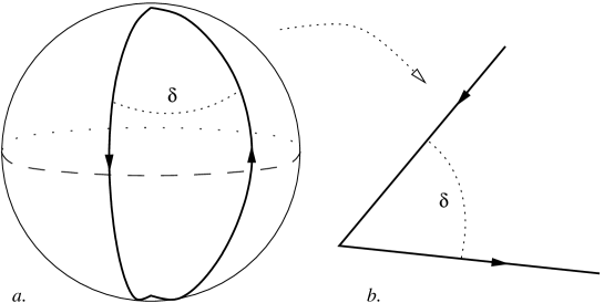
We shall therefore first find the string solution for a single cusp of angle $\delta$ in the plane and then we shall conformally transform it to the interesting system which is compact.

The cusp can be solved by using the conformal symmetry, as was done in [62]. Take the metric on $AdS_{3}\times S^{1}$ subspace of $AdS_{5}\times S^{5}$ to be

$$ds^{2}=\frac{L^{2}}{z^{2}}\left(dz^{2}+dr^{2}+r^{2}d\phi^{2}\right)+L^{2}d\varphi^{2}\,.$$ (C.5)

If the cusp is at the origin $r=0$, it is invariant under rescaling of $r$. This symmetry is then extended to the string world-sheet, where the $z$ coordinate will have a linear dependence on $r$. As world-sheet coordinates we take $r$ and $\phi$. The ansatz for the other coordinates is

$$z=r\,v(\phi)\,,\qquad\varphi=\varphi(\phi)\,.$$ (C.6)

The Nambu-Goto action is (prime is the derivative with respect to $\phi$)

$${\mathcal{S}}_{NG}=\frac{\sqrt{\lambda}}{2\pi}\int dr\,d\phi\frac{1}{r\,v^{2}}\sqrt{v^{\prime 2}+(1+v^{2})(1+v^{2}\varphi^{\prime 2})}\,.$$ (C.7)

The $r$ dependence is trivial and it is easy to find two conserved quantities, the energy and the canonical momentum conjugate to $\varphi$

$$E=\frac{1+v^{2}}{v^{2}\sqrt{v^{\prime 2}+(1+v^{2})(1+v^{2}\varphi^{\prime 2})}}\,,\qquad J=\frac{(1+v^{2})\varphi^{\prime}}{\sqrt{v^{\prime 2}+(1+v^{2})(1+v^{2}\varphi^{\prime 2})}}\,.$$ (C.8)

The BPS condition turns out, not surprisingly, to be $E=|J|$. To derive it consider the Legendre transform term which should be added to the action. Using the equations of motion it is

$${\mathcal{S}}_{L.T.}=\frac{\sqrt{\lambda}}{2\pi}\int dr\,d\phi\,(z\,p_{z})^{\prime}=\frac{\sqrt{\lambda}}{2\pi}\int dr\,d\phi\frac{-2-v^{\prime 2}-v^{2}(1+\varphi^{\prime 2})}{r\,v^{2}\sqrt{v^{\prime 2}+(1+v^{2})(1+v^{2}\varphi^{\prime 2})}}\,.$$ (C.9)

Requiring that the total Lagrangian vanishes locally leads to

$$v^{4}\varphi^{\prime 2}-1=0\,.$$ (C.10)

This can be written in terms of the conserved quantities in (C.8) as $E^{2}=J^{2}$.

The equation of motion for $v$ is

$$v^{\prime}=\frac{1+v^{2}}{v^{2}}\sqrt{p^{2}-v^{2}}\,,\qquad p=\frac{1}{E}\,.$$ (C.11)

which integrates to

$$\phi=\arcsin\frac{v}{p}-\frac{1}{\sqrt{1+p^{2}}}\arcsin\sqrt{\frac{1+1/p^{2}}{1+1/v^{2}}}\,.$$ (C.12)

This expression is valid over half the world-sheet, till the midpoint. Beyond that we should analytically continue to

$$\phi=\pi-\arcsin\frac{v}{p}-\frac{1}{\sqrt{1+p^{2}}}\left(\pi-\arcsin\sqrt{\frac{1+1/p^{2}}{1+1/v^{2}}}\right)\,,$$ (C.13)

The final value of $\phi$ when $v$ reaches zero again is

$$\delta=\pi\left(1-\frac{1}{\sqrt{1+p^{2}}}\right)\,.$$ (C.14)

The equation for $\varphi$ is even a bit simpler

$$\varphi^{\prime}=\pm\frac{1}{v^{2}}=\pm\frac{v^{\prime}}{(1+v^{2})\sqrt{p^{2}-v^{2}}}\,,$$ (C.15)

which integrates to

$$\varphi=\frac{1}{\sqrt{1+p^{2}}}\arcsin\sqrt{\frac{1+1/p^{2}}{1+1/v^{2}}}\,.$$ (C.16)

After going to the second branch the final value is

$$\varphi_{1}=\frac{\pi}{\sqrt{1+p^{2}}}\,,$$ (C.17)

and indeed $\delta+\varphi_{1}=\pi$, as should be the case by the supersymmetric construction of the scalar couplings (see (2.34) and the paragraph thereafter).

As mentioned above, the Nambu-Goto action is equal (up to a sign) to the total derivative which has to be added, so the full Lagrangian vanishes

$${\mathcal{S}}_{NG}=\frac{\sqrt{\lambda}}{2\pi}\int\frac{dr}{r}\int du\,\frac{-1}{p\,u^{2}}=\frac{\sqrt{\lambda}}{2\pi}\int\frac{dr}{r}\frac{1}{p\,u_{0}}\,,$$ (C.18)

with $u_{0}$ a cutoff. Note that for small $u$ the integrand $1/(rpu_{0})\sim 1/z_{0}$ is the standard divergence. Indeed it cancels against the Legendre transform.

The next step is to conformally transform to global $AdS$ with metric

$$ds^{2}=L^{2}\left[d\rho^{2}+\sinh^{2}\rho(d\theta^{2}+\sin^{2}\theta d\phi^{2})+d\varphi^{2}\right]\,,$$ (C.19)

by ($\phi$ and $\varphi$ are mapped to themselves)

$$\cosh\rho=\frac{1+z^{2}+r^{2}}{2z}\,,\qquad\sinh\rho\sin\theta=\frac{r}{z}\,.$$ (C.20)

This gives the surface

$$\cosh\rho=\frac{1+r^{2}+r^{2}v^{2}}{2rv}\,,\qquad\sinh\rho\sin\theta=\frac{1}{v}\,.$$ (C.21)

The relation between $v$, $\phi$ and $\varphi$ is as before, but the action will have to be calculated again using a different regularization that should give the expectation value of the Wilson loop with two cusps on the sphere.

Plugging in the solution into the Nambu-Goto action, it may be written in the following form

$${\mathcal{S}}_{NG} =\frac{\sqrt{\lambda}}{2\pi}\int\frac{dr}{r}\int d\phi\,\frac{p(1+v^{2})}{v^{4}}=\frac{\sqrt{\lambda}}{2\pi}\int\frac{dr}{r}\int dv\,\frac{p}{v^{2}\sqrt{p^{2}-v^{2}}}$$ (C.22)

$$=\frac{\sqrt{\lambda}}{2\pi}\int d\rho\,d\theta\,\frac{p\sinh^{2}\rho\sin\theta}{\sqrt{p^{2}\sinh^{2}\rho\sin^{2}\theta-1}}\,.$$

This expression is simple to integrate. For a fixed $\rho$ the variable $\theta$ varies between the two roots of $\sin\theta\sinh\rho=1/p$, and then back. Integrating over this variable gives $2\pi\sinh\rho$, so we are left with the $\rho$ integration between the minimal value, where $\sinh\rho=1/p$ and a cutoff $\rho_{0}$ at large $\rho$

$${\mathcal{S}}_{NG}=\sqrt{\lambda}\int d\rho\,\sinh\rho=\sqrt{\lambda}\left(\cosh\rho_{0}-\sqrt{1+\frac{1}{p^{2}}}\right)\,.$$ (C.23)

One may be tempted to simply throw away the divergent $\cosh\rho_{0}$ term, but some more care is actually required to proceed. As we noted before, the range of the $\theta$ integration for fixed $\rho_{0}$ is not $2\pi$, but roughly

$$2\pi-\frac{4}{p\sinh\rho_{0}}\,.$$ (C.24)

So this gives the possibility of some finite corrections left over from the divergent piece. The precise prescription for getting a finite value for the Wilson loop expectation value was given in [62]. It is defined in the Poincaré patch, where one can resort to considerations on the near horizon limit of D3-branes. The divergence in the bulk action is canceled by a boundary term which is a Legendre transform of the six coordinates orthogonal to the brane. In global $AdS$ this translates to

$${\mathcal{L}}_{\text{boundary}}=-\coth\rho_{0}\,p_{\rho}=-\coth\rho_{0}\,\rho^{\prime}\,\frac{\delta{\mathcal{L}}_{NG}}{\delta\rho^{\prime}}\,,$$ (C.25)

where $\rho^{\prime}$ is the derivative of $\rho$ with respect to the world-sheet coordinate orthogonal to the boundary. In the limit of large $\rho_{0}$ we can replace $\coth\rho_{0}\to 1$.

To evaluate it in practice one has to reintroduce $\rho^{\prime}$ into (C.22), where it was set to one, leading to the expression

$${\mathcal{S}}_{\text{boundary}} =-\frac{\sqrt{\lambda}}{2\pi}\int d\theta\,\frac{\sqrt{p^{2}\sinh^{2}\rho_{0}\sin^{2}\theta-1}}{p\sinh^{2}\rho_{0}\sin\theta}\left[\sinh^{2}\rho_{0}(1+\sin^{2}\theta(\partial_{\theta}\phi)^{2})+(\partial_{\theta}\varphi)^{2}\right]$$ (C.26)

$$=-\frac{\sqrt{\lambda}}{2\pi}\int d\theta\,\sin\theta\,\frac{p^{2}\sinh^{2}\rho_{0}(\sinh^{2}\rho_{0}\sin^{2}\theta+1)-\cosh^{2}\rho_{0}}{p(\sinh^{2}\rho_{0}\sin^{2}\theta+1)\sqrt{p^{2}\sinh^{2}\rho_{0}\sin^{2}\theta-1}}\,.$$

The first term in the numerator cancels part of the denominator giving the same integral over $\theta$ as in (C.22), which is equal to $2\pi\sinh\rho_{0}$. The second term, with $\cosh^{2}\rho_{0}$ in the numerator integrates to a finite answer such that the final result for the boundary term is

$${\mathcal{S}}_{\text{boundary}}\simeq-\sqrt{\lambda}\left(\sinh\rho_{0}-\frac{\coth\rho_{0}}{p\sqrt{1+p^{2}}}\right)\,.$$ (C.27)

Combining this with the bulk action (C.23), the divergences indeed cancel and we get the final answer for the action of the string dual to the two-longitudes Wilson loop

$${\mathcal{S}}=-\frac{p}{\sqrt{1+p^{2}}}\,\sqrt{\lambda}=-\frac{\sqrt{\lambda\,\delta(2\pi-\delta)}}{\pi}\,.$$ (C.28)

In the last equality we used (C.14) to represent $p$ in terms of $\delta$.

Non-BPS case

For completion we consider here the case of the general non-supersymmetric cusp in the plane with opening angle $\delta$ and arbitrary jump in the scalar coupling $\varphi_{1}$. This calculation is not used in the main text, as this loop is not BPS, but it was left unsolved in [62] and is a simple generalization of the BPS case.

In the supersymmetric case the ratio of the two conserved charges $J$ and $E$ in (C.8) was $\pm 1$. In the non-supersymmetric case it is still simple and we denote it by $q$

$$q\equiv\frac{J}{E}=v^{2}\varphi^{\prime}\,.$$ (C.29)

Using this we find the differential equation for $v$

$$v^{\prime 2}=\frac{1+v^{2}}{v^{4}}[p^{2}+(p^{2}-q^{2})v^{2}-v^{4}]\,,\qquad p=\frac{1}{E}\,.$$ (C.30)

This is an elliptic equation. To see that define

$$\zeta=\sqrt{\frac{v^{2}(1+b^{2})}{b^{2}(1+v^{2})}}\,,\qquad b^{2}=\frac{1}{2}\left(p^{2}-q^{2}+\sqrt{(p^{2}-q^{2})^{2}+4p^{2}}\right)\,.$$ (C.31)

Then $\zeta$ satisfies

$$\zeta^{\prime 2}=\frac{p^{2}}{b^{2}}\left(1-\frac{1+b^{2}}{b^{2}\zeta^{2}}\right)^{2}(1-\zeta^{2})(1-k^{2}\zeta^{2})\,,\qquad k^{2}=\frac{b^{2}(p^{2}-b^{2})}{p^{2}(1+b^{2})}\,.$$ (C.32)

Therefore the relation between $\zeta$ and $\phi$ is given in terms of incomplete elliptic integrals of the first and third kind $F$ and $\Pi$ with argument $\arcsin\zeta$ and modulus $k$

$$\phi=\frac{b}{p\sqrt{1+b^{2}}}\left[F(\arcsin\zeta;k)-\Pi\left(\frac{b^{2}}{1+b^{2}},\arcsin\zeta;k\right)\right]\,.$$ (C.33)

At the boundary $v=0$ so also $\zeta=0$. It reaches a maximal value $\zeta=1$ beyond which another copy of the surface continues with

$$\phi=\frac{b}{p\sqrt{1+b^{2}}}\left[2K(k)-2\Pi\left(\frac{b^{2}}{1+b^{2}};k\right)-F(\arcsin\zeta;k)+\Pi\left(\frac{b^{2}}{1+b^{2}},\arcsin\zeta;k\right)\right]\,.$$ (C.34)

The final value of $\phi$ when we reach the boundary again is twice the complete elliptic integrals

$$\delta=\frac{2b}{p\sqrt{1+b^{2}}}\left[K(k)-\Pi\left(\frac{b^{2}}{1+b^{2}};k\right)\right]\,.$$ (C.35)

Integrating $\varphi$ leads to an even simpler expression in terms of elliptic integrals of the first kind

$$\varphi=\int d\phi\,\frac{q}{v^{2}}=\frac{q\,b}{p\sqrt{1+b^{2}}}F(\arcsin\zeta;k)\,.$$ (C.36)

The final value of $\varphi$ is again related to the complete integral

$$\varphi=2\frac{q\,b}{p\sqrt{1+b^{2}}}K(k)\,.$$ (C.37)

Then we can calculate the classical action

$${\mathcal{S}} =\frac{\sqrt{\lambda}}{2\pi}\int dr\,d\phi\,\frac{p}{r}\frac{1+v^{2}}{v^{4}}$$ (C.38)

$$=\frac{\sqrt{\lambda}}{2\pi}\int\frac{dr}{r}\frac{\sqrt{1+b^{2}}}{b}\left[-\frac{\sqrt{(1-\zeta^{2})(1-k^{2}\zeta^{2})}}{\zeta}+\left[F(\arcsin\zeta;k)-E(\arcsin\zeta;k)\right]\right]\,,$$

where $E$ denotes an elliptic integral of the second kind. The right hand side should be evaluated at the two boundaries where $\zeta=0$ (on the two branches). The result is

$${\mathcal{S}}_{NG}=\frac{\sqrt{\lambda}}{2\pi}\int\frac{dr}{r}\frac{\sqrt{1+b^{2}}}{b}\left[\frac{2}{\zeta_{0}}+2\left[K(k)-E(k)\right]\right]\,.$$ (C.39)

Here $\zeta_{0}$ is a cutoff at small $\zeta$, so the first term is equal to

$$\frac{\sqrt{\lambda}}{2\pi}\int dr\frac{2\sqrt{1+b^{2}}}{b\,r\zeta_{0}}=\frac{\sqrt{\lambda}}{2\pi}\int dr\frac{2}{z_{0}}\,,$$ (C.40)

where $z_{0}$ is a cutoff on $z$, and this is the standard divergence for the two rays making the cusp. The divergence is canceled as usual by a boundary term.

C.3 Toroidal loops

We describe now the toroidal loops introduced in Section 2.4 and Section 2.5. We perform the calculation in the general case where the radii of the loops $r_{1}$ and $r_{2}$ are independent of the periods $k_{1}$ and $k_{2}$ along the two cycles of the torus. To focus on the case of the latitude on the Hopf base discussed in Section 2.4, one should simply set

$$\sin{\theta\over 2}=\sqrt{\frac{k_{2}}{k_{1}+k_{2}}}\,.$$ (C.41)

Consider a doubly-periodic motion on $S^{3}$

$$x_{1}=\sin\frac{\theta}{2}\sin k_{1}t\,,\quad x_{2}=\sin\frac{\theta}{2}\cos k_{1}t\,,\quad x_{3}=\cos\frac{\theta}{2}\sin k_{2}t\,,\quad x_{4}=\cos\frac{\theta}{2}\cos k_{2}t\,,$$ (C.42)

where $\theta$ is one of the Euler angles, while the other two angles are given by

$$\phi=(k_{1}+k_{2})t\,,\qquad\psi=(k_{2}-k_{1})t\,.$$ (C.43)

The scalar couplings for these loops are simple

$$\frac{1}{2}\,\sigma_{1}^{R} =\frac{1}{2}(k_{1}+k_{2})\sin\theta\,\cos(k_{2}-k_{1})t\,dt\,,$$ (C.44)

$$\frac{1}{2}\,\sigma_{2}^{R} =\frac{1}{2}(k_{1}+k_{2})\sin\theta\,\sin(k_{2}-k_{1})t\,dt\,,$$

$$\frac{1}{2}\,\sigma_{3}^{R} =\left(k_{2}\cos^{2}\frac{\theta}{2}-k_{1}\sin^{2}\frac{\theta}{2}\right)dt\,.$$

This is just a periodic motion, as in the case of the latitude on the great $S^{2}$.

It is possible to find the minimal surface representing this Wilson loop in $AdS_{5}\times S^{5}$ using the techniques of [60]. There it was shown how to calculate a general periodic Wilson loop, but the example of motion on a torus was not done explicitly.

One first notices that the $AdS_{5}$ and $S^{5}$ parts of the $\sigma$-model completely decouple. In principle the two systems may be coupled because of the Virasoro constraint, which should be satisfied on the combined system only. All the examples in [60] where this occurred were the correlation functions of two loops. Here we have a single loop and in this case the Virasoro constraint is indeed satisfied independently on both sides.

The solution to the equations of motion on the $S^{5}$ side are like in the latitude on the great $S^{2}$ example (C.2)

$$\sin\vartheta=\frac{1}{\cosh[(k_{2}-k_{1})(\sigma_{0}\pm\sigma)]}\,,\qquad\varphi=(k_{2}-k_{1})\tau\,.$$ (C.45)

The sign choice corresponds to a surface wrapping the northern or southern hemisphere and the integration constant $\sigma_{0}$ is chosen so that at $\sigma=0$ it reaches the boundary value

$$\sin\vartheta_{0}=\frac{1}{\cosh[(k_{2}-k_{1})\sigma_{0}]}=\frac{(k_{1}+k_{2})\sin\theta}{2\sqrt{k_{1}^{2}\sin^{2}\frac{\theta}{2}+k_{2}^{2}\cos^{2}\frac{\theta}{2}}}\,.$$ (C.46)

The action for the string will be the sum of $AdS_{5}$ part and of the $S^{5}$ part. The latter is just the area of the part of the sphere covered by the string (taking $k_{2}\geq k_{1}$)

$${\mathcal{S}}_{S^{5}} =\left(k_{2}-k_{1}\right)\left(1\pm\frac{k_{2}\cos^{2}\frac{\theta}{2}-k_{1}\sin^{2}\frac{\theta}{2}}{\sqrt{k_{1}^{2}\sin^{2}\frac{\theta}{2}+k_{2}^{2}\cos^{2}\frac{\theta}{2}}}\right)\sqrt{\lambda}$$ (C.47)

$$=\left(k_{2}-k_{1}\pm\sqrt{k_{1}^{2}\sin^{2}\frac{\theta}{2}+k_{2}^{2}\cos^{2}\frac{\theta}{2}}\mp\frac{k_{1}k_{2}}{\sqrt{k_{1}^{2}\sin^{2}\frac{\theta}{2}+k_{2}^{2}\cos^{2}\frac{\theta}{2}}}\right)\sqrt{\lambda}\,.$$

The sign choice again corresponds to the two possible wrappings of $S^{2}$.

To solve the $AdS_{5}$ part it is convenient to write it as a hypersurface in flat six-dimensional Minkowski space

$$-Y_{0}^{2}+Y_{1}^{2}+Y_{2}^{2}+Y_{3}^{2}+Y_{4}^{2}+Y_{5}^{2}=-L^{2}\,.$$ (C.48)

Now let us define the coordinates $r_{0}$, $r_{1}$, $r_{2}$, $v$, $\phi_{1}$ and $\phi_{2}$ by

$$Y_{0}=Lr_{0}\cosh v\,,\qquad Y_{5}=Lr_{0}\sinh v\,,$$ (C.49)

$$Y_{1}=Lr_{1}\cos\phi_{1}\,,\qquad Y_{2}=Lr_{1}\sin\phi_{1}\,,$$

$$Y_{3}=Lr_{2}\cos\phi_{2}\,,\qquad Y_{4}=Lr_{2}\sin\phi_{2}\,.$$

Those coordinates satisfy the constraint $-r_{0}^{2}+r_{1}^{2}+r_{2}^{2}=-1$, and the metric of the embedding flat Minkowski space is

$$ds^{2}=L^{2}\left(-dr_{0}^{2}+r_{0}^{2}dv^{2}+dr_{1}^{2}+r_{1}^{2}d\phi_{1}^{2}+dr_{2}^{2}+r_{2}^{2}d\phi_{2}^{2}\right)\,.$$ (C.50)

The relevant ansatz for our system of periodic motion on $T^{2}$ is

$$r_{i}=r_{i}(\sigma)\,,\qquad v=v(\sigma)\,,\qquad\phi_{1}=k_{1}\tau+\alpha_{1}(\sigma)\,,\qquad\phi_{2}=k_{2}\tau+\alpha_{2}(\sigma)\,.$$ (C.51)

Furthermore we can set $\alpha_{1}$, $\alpha_{2}$ and $v$ to be constants, leaving only the action for $r_{0}$, $r_{1}$, and $r_{2}$

$${\mathcal{S}}_{AdS_{5}}=\frac{L^{2}}{4\pi\alpha^{\prime}}\int d\sigma\,d\tau\big{[}-r_{0}^{\prime 2}+r_{1}^{\prime 2}+r_{2}^{\prime 2}+r_{1}^{2}k_{1}^{2}+r_{2}^{2}k_{2}^{2}+\Lambda\left(-r_{0}^{2}+r_{1}^{2}+r_{2}^{2}+1\right)\big{]}\,.$$ (C.52)

Here $\Lambda$ is a Lagrange multiplier.

The equations of motion for $r_{0}$, $r_{1}$ and $r_{2}$ are

$$r_{0}^{\prime\prime}=\Lambda r_{0}\,,\qquad r_{1}^{\prime\prime}=(k_{1}^{2}+\Lambda)r_{1}\,,\qquad r_{2}^{\prime\prime}=(k_{2}^{2}+\Lambda)r_{2}\,.$$ (C.53)

It is simple to find the first integral of motion, it is the diagonal component of the $AdS_{5}$ contribution to the stress-energy tensor

$$-r_{0}^{\prime 2}+r_{1}^{\prime 2}+r_{2}^{\prime 2}-k_{1}^{2}r_{1}^{2}-k_{2}^{2}r_{2}^{2}=0\,.$$ (C.54)

Using the Virasoro constraint, the classical action is twice the kinetic piece

$${\mathcal{S}}_{AdS_{5}}=2{\mathcal{S}}_{AdS_{5}}^{kinetic}=\frac{\sqrt{\lambda}}{2\pi}\int d\sigma\,d\tau\left(r_{1}^{2}k_{1}^{2}+r_{2}^{2}k_{2}^{2}\right)\,.$$ (C.55)

The other integrals of motion are

$$I_{0}= r_{0}^{2}-\frac{1}{k_{1}^{2}}(r_{0}r_{1}^{\prime}-r_{1}r_{0}^{\prime})^{2}-\frac{1}{k_{2}^{2}}(r_{0}r_{2}^{\prime}-r_{2}r_{0}^{\prime})^{2}\,,$$ (C.56)

$$I_{1}= r_{1}^{2}-\frac{1}{k_{1}^{2}}(r_{0}r_{1}^{\prime}-r_{1}r_{0}^{\prime})^{2}+\frac{1}{k_{1}^{2}-k_{2}^{2}}(r_{1}r_{2}^{\prime}-r_{2}r_{1}^{\prime})^{2}\,.$$

We can define $I_{2}$ in a similar fashion, but it is not an independent integral, since $-I_{0}+I_{1}+I_{2}=-1$.

We know that the range of the world-sheet coordinate $\sigma$ is infinite (from the $S^{5}$ part of the solution), and that for large $\sigma$ both $r_{1}$ and $r_{2}$ vanish (as well as their derivatives), while $r_{0}\to 1$. From this we easily conclude that the integration constants are $I_{0}=1$ and $I_{1}=I_{2}=0$.

To solve these equations we define the coordinates $\zeta_{1}$ and $\zeta_{2}$ which are the roots of the equation

$$\frac{r_{0}^{2}}{\zeta_{i}^{2}}-\frac{r_{1}^{2}}{\zeta_{i}^{2}-k_{1}^{2}}-\frac{r_{2}^{2}}{\zeta_{i}^{2}-k_{2}^{2}}=0\,,$$ (C.57)

and we find

$$r_{0}=\frac{\zeta_{1}\zeta_{2}}{k_{1}k_{2}}\,,\qquad r_{1}=\sqrt{\frac{(\zeta_{1}^{2}-k_{1}^{2})(\zeta_{2}^{2}-k_{1}^{2})}{k_{1}^{2}(k_{2}^{2}-k_{1}^{2})}}\,,\qquad r_{2}=\sqrt{\frac{(\zeta_{1}^{2}-k_{2}^{2})(\zeta_{2}^{2}-k_{2}^{2})}{k_{2}^{2}(k_{1}^{2}-k_{2}^{2})}}\,.$$ (C.58)

The integrals of motion $I_{0}$ and $I_{1}$ lead to the equations

$$\zeta_{1}^{\prime}=\pm\frac{(\zeta_{1}^{2}-k_{1}^{2})(\zeta_{1}^{2}-k_{2}^{2})}{\zeta_{1}^{2}-\zeta_{2}^{2}}\,,\qquad\zeta_{2}^{\prime}=\pm\frac{(\zeta_{2}^{2}-k_{1}^{2})(\zeta_{2}^{2}-k_{2}^{2})}{\zeta_{1}^{2}-\zeta_{2}^{2}}\,.$$ (C.59)

The ratio of those two equations is then simple to integrate. If we assume without loss of generality that $k_{1}<k_{2}$, then it turns out that for our system we can take $k_{1}\leq\zeta_{1}\leq k_{2}\leq\zeta_{2}$ and in the first equation in (C.59) there should be the negative sign while in the second the positive one. The solution is given in terms of a constant $c$

$$k_{1}\,\hbox{arctanh}\,\frac{\zeta_{1}}{k_{2}}-k_{2}\,\hbox{arccoth}\,\frac{\zeta_{1}}{k_{1}}+k_{1}\,\hbox{arccoth}\,\frac{\zeta_{2}}{k_{2}}-k_{2}\,\hbox{arccoth}\,\frac{\zeta_{2}}{k_{1}}=c\,.$$ (C.60)

or

$$\left(\frac{(\zeta_{1}-k_{1})(\zeta_{2}+k_{1})}{(\zeta_{1}+k_{1})(\zeta_{2}-k_{1})}\right)^{k_{2}}\left(\frac{(k_{2}+\zeta_{1})(\zeta_{2}-k_{2})}{(k_{2}-\zeta_{1})(\zeta_{2}+k_{2})}\right)^{k_{1}}=C\,.$$ (C.61)

Note that this solution is valid for any torus. The radii $\sin\theta/2$ and $\cos\theta/2$ are encoded in the asymptotic values of $r_{1}$ and $r_{2}$ whose ratio should approach $\tan(\theta/2)$. In terms of the $\zeta$’s, this corresponds to one of them ($\zeta_{1}$) approaching the constant $k_{1}k_{2}/\sqrt{k_{1}^{2}\sin^{2}(\theta/2)+k_{2}^{2}\cos^{2}(\theta/2)}$, while $\zeta_{2}$ diverges.

So our solution has $\zeta_{1}$ starting at this constant near the boundary of $AdS_{5}$ and decreasing to $k_{1}$, while $\zeta_{2}$ will start at infinity and decrease to $k_{2}$. The constant $C$ in (C.61) is

$$\left(\frac{k_{2}-\sqrt{k_{1}^{2}\sin^{2}\frac{\theta}{2}+k_{2}^{2}\cos^{2}\frac{\theta}{2}}}{k_{2}+\sqrt{k_{1}^{2}\sin^{2}\frac{\theta}{2}+k_{2}^{2}\cos^{2}\frac{\theta}{2}}}\right)^{k_{2}}\left(\frac{\sqrt{k_{1}^{2}\sin^{2}\frac{\theta}{2}+k_{2}^{2}\cos^{2}\frac{\theta}{2}}+k_{1}}{\sqrt{k_{1}^{2}\sin^{2}\frac{\theta}{2}+k_{2}^{2}\cos^{2}\frac{\theta}{2}}-k_{1}}\right)^{k_{1}}.$$ (C.62)

Is is not easy to solve for the $\zeta$’s (or $r$’s) in terms of $\sigma$, but that turns out not to be necessary. The action can be evaluated without that

$${\mathcal{S}}_{AdS_{5}} =\frac{\sqrt{\lambda}}{2\pi}\int d\sigma\,d\tau\,(-r_{0}^{\prime 2}+r_{1}^{\prime 2}+r_{2}^{\prime 2})$$ (C.63)

$$=\sqrt{\lambda}\int d\sigma\,\left(\frac{\zeta_{1}^{\prime 2}(\zeta_{2}^{2}-\zeta_{1}^{2})}{(\zeta_{1}^{2}-k_{1}^{2})(k_{2}^{2}-\zeta_{1}^{2})}+\frac{\zeta_{2}^{\prime 2}(\zeta_{2}^{2}-\zeta_{1}^{2})}{(\zeta_{2}^{2}-k_{1}^{2})(\zeta_{2}^{2}-k_{2}^{2})}\right)$$

$$=-\sqrt{\lambda}\left(\int_{\frac{k_{1}k_{2}}{\sqrt{k_{1}^{2}\sin^{2}\frac{\theta}{2}+k_{2}^{2}\cos^{2}\frac{\theta}{2}}}}^{k_{1}}d\zeta_{1}+\int_{\infty}^{k_{2}}d\zeta_{2}\right)$$

$$\simeq-\sqrt{\lambda}\left(k_{1}+k_{2}-\frac{k_{1}k_{2}}{\sqrt{k_{1}^{2}\sin^{2}\frac{\theta}{2}+k_{2}^{2}\cos^{2}\frac{\theta}{2}}}\right)\,.$$

In the last expression the divergence was removed.

Together with the $S^{5}$ part (C.47) one gets the total action

$${\mathcal{S}}=\left(-2k_{1}\pm\sqrt{k_{1}^{2}\sin^{2}\frac{\theta}{2}+k_{2}^{2}\cos^{2}\frac{\theta}{2}}+(1\mp 1)\frac{k_{1}k_{2}}{\sqrt{k_{1}^{2}\sin^{2}\frac{\theta}{2}+k_{2}^{2}\cos^{2}\frac{\theta}{2}}}\right)\sqrt{\lambda}\,.$$ (C.64)

Appendix D Almost complex structure for $S^{2}$ and $S^{6}$

In this appendix we provide an alternative, more geometrical understanding of the origin of the almost complex structure ${\cal J}$. The main clue comes from observing that our string solutions satisfy

$$x^{2}+z^{2}=1\,,$$ (D.1)

and therefore reside inside an $AdS_{4}\times S^{2}$ subspace of $AdS_{5}\times S^{5}$ . It is then natural to look for an almost complex structure on this subspace. To understand how this observation can help we note that we could rewrite equation (D.1) as $x^{\mu}x^{\mu}+z^{4}y^{i}y^{i}=1$, which, up to a $z$ factor, is analogous to the equation of a 6-sphere embedded in $(x^{\mu},y^{i})$. It will be therefore insightful to review how we can construct an almost complex structure on $S^{6}$ in $\mathbb{R}^{7}$. To understand how to proceed let us begin with a simpler case, which is the construction of an almost complex structure on $S^{2}$. This structure is by definition a linear endomorphism on the tangent space of the sphere which satisfies

$$J:TS^{2}\rightarrow TS^{2},\qquad J^{2}=-1.$$ (D.2)

In terms of the usual embedding of the sphere in $\mathbb{R}^{3}$ let us consider the following linear operator

$$J=\left(\begin{array}[]{ccc}0&-x_{3}&x_{2}\\ x_{3}&0&-x_{1}\\ -x_{2}&x_{1}&0\\ \end{array}\right).$$ (D.3)

This $J$ defines an almost complex structure on $S^{2}$. To see that we first observe that $J$ is a well defined map on $TS^{2}$ because for any $\vec{p}=(p_{1},p_{2},p_{3})$ in the tangent space of $\vec{x}=(x_{1},x_{2},x_{3})$ we have $J(\vec{p})\cdot{\vec{x}}=0$. This says that $J(\vec{p})$ is orthogonal to $\vec{x}$ and therefore $J$ maps tangent vectors into tangent vectors. For $J$ to be an almost complex structure it remains to prove that it squares to minus the identity, and indeed

$$J^{2}(p)=\left(\begin{array}[]{c}-p_{1}+x_{1}\,x\cdot p\\ -p_{2}+x_{2}\,x\cdot p\\ -p_{3}+x_{3}\,x\cdot p\\ \end{array}\right)=-\left(\begin{array}[]{c}p_{1}\\ p_{2}\\ p_{3}\\ \end{array}\right).$$ (D.4)

Note that the action of $J$ on $\vec{p}$ can be simply thought of as the cross product $\vec{x}\times\vec{p}$ .

Let us try to extend this construction. It is a fact that the only spheres which admit an almost complex structure are $S^{2}$ (in which case $J$ is also integrable) and $S^{6}$. The construction of an almost complex structure for the latter case can be carried over in analogy to what done for the unit 2-sphere if we work with the octonion algebra $\mathbb{O}$. An octonion element can be written as

$${\bf x}=x_{0}+x_{1}{\bf e}_{1}+x_{2}{\bf e}_{2}+x_{3}{\bf e}_{3}+x_{4}{\bf e}_{4}+x_{5}{\bf e}_{5}+x_{6}{\bf e}_{6}+x_{7}{\bf e}_{7}$$ (D.5)

where the algebra generators satisfy

$${\bf e}_{i}^{2}=-1,\qquad{\bf e}_{i}{\bf e}_{j}=-{\bf e}_{j}\,{\bf e}_{i}.$$ (D.6)

We can think of $S^{6}$ as the hypersurface $|x|=1$ with $x\in\rm{Im}\,\mathbb{O}$, the imaginary octonions being obtained by setting $x_{0}=0$. We will see that $S^{6}$, when considered as the set of unit norm imaginary octonions, inherits an almost complex structure from the octonion multiplication [82].

If we want to construct an almost complex structure on $S^{6}$ using the analogy with $S^{2}$ we need to define a cross product. Luckily a cross product between two vectors, satisfying all the usual assumptions, exists only in dimensions 3 and 7. The cross product between two octonions ${\bf x}$ and ${\bf y}$ is defined as

$${\bf x}\times{\bf y}=\frac{1}{2}({\bf x}{\bf y}-{\bf y}{\bf x})={\rm Im}\left({\bf x}{\bf y}\right)$$ (D.7)

where ${\bf x}{\bf y}$ is the non-commutative and non-associative octonion product. If we work with imaginary octonions the cross product reduces to the ordinary octonion multiplication. The claim is that an almost complex structure $J$ can be constructed as

$$J={x}\times{p}\,,\qquad{x}\in S^{6},\qquad{p}\in T_{x}S^{6}$$ (D.8)

where ${x}=(x_{1},x_{2},x_{3},x_{4},x_{5},x_{6},x_{7})$ and ${p}=(p_{1},p_{2},p_{3},p_{4},p_{5},p_{6},p_{7})$ are thought of as imaginary octonions. Using a particular choice for the multiplication table one gets the following matrix

$$J=\left(\begin{array}[]{ccccccc}0&-x_{7}&x_{6}&x_{5}&-x_{4}&-x_{3}&x_{2}\\ x_{7}&0&-x_{5}&x_{6}&x_{3}&-x_{4}&-x_{1}\\ -x_{6}&x_{5}&0&x_{7}&-x_{2}&x_{1}&-x_{4}\\ -x_{5}&-x_{6}&-x_{7}&0&x_{1}&x_{2}&x_{3}\\ x_{4}&-x_{3}&x_{2}&-x_{1}&0&x_{7}&-x_{6}\\ x_{3}&x_{4}&-x_{1}&-x_{2}&-x_{7}&0&x_{5}\\ -x_{2}&x_{1}&x_{4}&-x_{3}&x_{6}&-x_{5}&0\end{array}\right)$$ (D.9)

In complete analogy to the $S^{2}$ case we can show that $J$ defines linear endomorphism on the tangent space and that $J^{2}({p})=-{p}$ for any tangent vector ${p}$. This proves we have constructed an almost complex structure on the unit 6-sphere. Using a notation similar to (3.20) we can write the matrix $J^{i}_{\ j}$ as

$$J^{i}_{\ j}=J^{i}_{\ j;\,k}\,x^{k}.$$ (D.10)

Note that up to $z$ factors, $J$ coincides with the almost complex structure ${\cal J}$ associated to the Wilson loops, see (3.23), after the relabeling $x_{5}\rightarrow-y_{1},\,x_{6}\rightarrow-y_{2},\,x_{7}\rightarrow-y_{3}$. The corresponding fundamental two-form reads

$$J=\frac{1}{2}\,J_{MN}\,dx^{M}\wedge dx^{N}$$

$$=x_{1}(dx_{72}+dx_{36}+dx_{45})+x_{2}(dx_{17}+dx_{53}+dx_{46})+x_{3}(dx_{61}+dx_{25}+dx_{47})$$

$$+x_{4}(dx_{51}+dx_{62}+dx_{73})+x_{5}(dx_{14}+dx_{32}+dx_{67})+x_{6}(dx_{13}+dx_{24}+dx_{75})$$

$$+x_{7}(dx_{21}+dx_{34}+dx_{56}).$$ (D.11)

Note that, as was the case for ${\cal J}$, this two-form is not closed but rather we have

$$dJ=3(dx_{172}+dx_{136}+dx_{145}+dx_{325}+dx_{246}+dx_{347}+dx_{567}).$$ (D.12)

This form is the associative three-form $\phi$ preserved by the $G_{2}$ group. The explanation for the appearance of $\phi$ in this context is that $G_{2}\subset SO(7)$ is the automorphism group of the octonions. The reason for which $dJ\neq 0$ is the well known fact that $S^{6}$ is not Kähler.

Appendix E 2-dimensional YM in the WML $\xi=-1$ gauge

In this appendix we present an explicit computation in the $\xi=-1$ generalized Feynman gauge with WML prescription for the two-dimensional near-flat limit discussed in Section 4.1.1. Since we know that the non-interacting graphs from our Wilson loops in four dimensions in the Feynman gauge agree with the 2-dimensional propagators in this gauge, we turned to the first interacting graphs, which appear at order $\lambda^{2}$.

While we were not able to find agreement between the interacting graphs in four dimensions and two dimensions for a general loop, we present the calculation here nonetheless in the hope that it would aid in future explorations of the subject. To get some concrete results we focused on the one case where the interacting graphs were calculated in four dimensions—the circular loop. In this special example the two propagators in the $\xi=-1$ gauge sum up to the (single) propagator in the light-cone gauge, hence the ladder diagrams in the two gauges are equal. In the light-cone gauge there are no interactions and therefore in our gauge the interaction graphs for the circle should all cancel, which we indeed verify.

We start by deriving the Feynman rules in this generalized gauge in the near-flat limit. The Euclidean action reads

$$L=\frac{1}{g_{2d}^{2}}\left[\frac{1}{4}\left(F_{rs}^{a}\right)^{2}+\frac{1}{2\xi}\left(\partial_{r}A^{a,r}\right)^{2}+\partial_{r}b^{a}\left(D^{r}c\right)^{a}\right]\,,$$ (E.1)

where $r,s=1,2$ and

$$F^{a}_{rs}=\partial_{[r}A^{a}_{s]}+f^{abc}A^{b}_{r}\,A^{c}_{s}\,,\qquad\left(D_{r}c\right)^{a}=\partial_{r}c^{a}+f^{abc}A^{b}_{r}\,c^{c}\,.$$ (E.2)

Choosing the gauge $\xi=-1$ and using the light-cone coordinates $x^{\pm}=\frac{1}{2}(x^{1}\pm ix^{2})$ (so that the metric is $g_{+-}=2$) the action becomes

$$L = \frac{1}{g_{2d}^{2}}\bigg{[}-\frac{1}{4}(\partial_{+}A_{-}^{a})^{2}-\frac{1}{4}(\partial_{-}A_{+}^{a})^{2}-b^{a}\partial_{+}\partial_{-}c^{a}$$ (E.5)

$$\hskip 22.76228pt+\frac{1}{4}f^{abc}(\partial_{+}A^{a}_{-}-\partial_{-}A^{a}_{+})A^{b}_{-}A^{c}_{+}-\frac{1}{8}f^{abc}f^{ade}A^{b}_{+}A^{c}_{-}A^{d}_{+}A^{e}_{-}$$

$$\hskip 22.76228pt+\frac{1}{2}f^{abc}(\partial_{+}b^{a})A_{-}^{b}c^{c}+\frac{1}{2}f^{abc}(\partial_{-}b^{a})A_{+}^{b}c^{c}\bigg{]}\,.$$

The propagators for the gauge fields in the WML prescription are then

$$\Delta^{ab}_{++}(x,y)\equiv\delta^{ab}\Delta_{++}(x,y)=\delta^{ab}\frac{g_{2d}^{2}}{2\pi}\frac{x^{-}-y^{-}}{x^{+}-y^{+}}\,,$$ (E.6)

$$\Delta^{ab}_{--}(x,y)\equiv\delta^{ab}\Delta_{--}(x,y)=\delta^{ab}\frac{g_{2d}^{2}}{2\pi}\frac{x^{+}-y^{+}}{x^{-}-y^{-}}\,,$$ (E.7)

where the normalization is fixed by requesting

$$\frac{1}{2g_{2d}^{2}}\partial^{2}_{x^{-}}\Delta_{++}(x,y)=\delta^{2}(x-y)\,,$$ (E.8)

and similarly for $\Delta_{--}$. For the ghosts one has

$$\Delta_{gh}^{ab}(x,y)\equiv\delta^{ab}\Delta_{gh}(x,y)=-\delta^{ab}\frac{g_{2d}^{2}}{4\pi}\log(x-y)^{2}\,.$$ (E.9)

The vertices can be easily read off from the action.

E.1 Three-point graphs

We now write down the interacting graphs starting with the ones with an internal 3-vertex. On the loop there can be two $A_{+}$’s and one $A_{-}$ or two $A_{-}$’s and one $A_{+}$. These two cases are one the complex conjugate of the other so it is sufficient to compute only one of them, say the first one, which we denote $\Sigma^{(3)}_{++-}$. Expanding the action $e^{-S}$ to first order and the Wilson loop to third order, one obtains after performing all the Wick contractions

$$\Sigma^{(3)}_{++-}=-\frac{i^{3}}{3!N}\frac{1}{4g_{2d}^{2}}\frac{iN(N^{2}-1)}{4}\oint d\tau_{1}d\tau_{2}d\tau_{3}\,\varepsilon(\tau_{1}\tau_{2}\tau_{3})\int d^{2}y\,\times$$ (E.10)

$$\hskip 28.45274pt\times\bigg{\{}\dot{x}^{+}_{1}\dot{x}^{+}_{2}\dot{x}^{-}_{3}\Delta_{--}(y,x_{3})\Big{[}\Delta_{++}(y,x_{2})\partial_{y^{-}}\Delta_{++}(y,x_{1})-\Delta_{++}(y,x_{1})\partial_{y^{-}}\Delta_{++}(y,x_{2})\Big{]}$$ (E.11)

$$\hskip 85.35826pt-(1\leftrightarrow 3)-(2\leftrightarrow 3)\bigg{\}}\,.$$ (E.12)

Here we have used that ${\rm Tr\,}(T^{a}T^{b}T^{c})f^{abc}=\frac{i}{4}N(N^{2}-1)$ and the symbol $\varepsilon(\tau_{1}\tau_{2}\tau_{3})$ enforces the path ordering through the antisymmetrization of $\tau_{1}$, $\tau_{2}$, and $\tau_{3}$.

We now proceed with the integration over $y$. The first term in curly brackets can be explicitly written (up to the $\dot{x}^{+}_{1}\dot{x}^{+}_{2}\dot{x}^{-}_{3}$ structure and the constant factors in the propagators which we do not include) as

$$\int d^{2}y\,\frac{(y^{+}-x^{+}_{3})(x^{-}_{1}-x^{-}_{2})}{(y^{-}-x^{-}_{3})(y^{+}-x^{+}_{1})(y^{+}-x^{+}_{2})}=$$ (E.13)

$$\hskip 28.45274pt=\frac{x^{-}_{1}-x^{-}_{2}}{x^{+}_{1}-x^{+}_{2}}\int d^{2}y\left(\frac{x^{+}_{1}-x^{+}_{3}}{(y^{-}-x^{-}_{3})(y^{+}-x^{+}_{1})}-\frac{x^{+}_{2}-x^{+}_{3}}{(y^{-}-x^{-}_{3})(y^{+}-x^{+}_{2})}\right)\,.$$ (E.14)

It is convenient to parametrize the position of the vertex as $y^{\pm}\equiv\frac{\rho}{2}e^{\pm i\phi}$. The integrals in $\phi$ are of the type

$$\int_{0}^{2\pi}\frac{d\phi}{\left(e^{-i\phi}-a\right)\left(e^{i\phi}-b\right)}=\frac{2\pi}{ab-1}\left[\vartheta(|a|-1)-\vartheta(1-|b|)\right]\,,$$ (E.15)

where $a,b\in\mathbb{C}$ and $\vartheta$ is the step function. This identity can be easily proven starting from

$$\int_{0}^{2\pi}\frac{d\phi}{e^{i\phi}-a}=-\frac{2\pi}{a}\vartheta(|a|-1)\,.$$ (E.16)

After integrating over $\phi$, equation (E.14) becomes

$$8\pi\frac{(x^{-}_{1}-x^{-}_{2})(x^{+}_{1}-x^{+}_{3})}{x^{+}_{1}-x^{+}_{2}}\int_{0}^{R}\frac{\rho\,d\rho}{4x^{-}_{3}x^{+}_{1}-\rho^{2}}\left[\vartheta(r(\tau_{3})-\rho)-\vartheta(\rho-r(\tau_{1}))\right]-(1\leftrightarrow 2)\,,$$ (E.17)

where we have introduced an IR cutoff $R$ and parametrized $x^{\pm}_{i}\equiv\frac{r(\tau_{i})}{2}e^{\pm i\tau_{i}}$. For convenience, we will use in the following the shorthand notation $r_{i}\equiv r(\tau_{i})$. The integral above can be easily performed and yields

$$4\pi\frac{(x^{-}_{1}-x^{-}_{2})(x^{+}_{1}-x^{+}_{3})}{x^{+}_{1}-x^{+}_{2}}\log\left(\frac{R^{2}-4x^{-}_{3}x^{+}_{1}}{r_{1}^{2}+r_{3}^{2}-2r_{1}r_{3}\cos\tau_{13}}\right)-(1\leftrightarrow 2)\,,$$ (E.19)

where we have also introduced the notation $\tau_{ij}\equiv\tau_{i}-\tau_{j}$. Including all the prefactors in equation (E.12) and summing over the permutations yields the final result

$$\Sigma^{(3)}_{++-}=-\frac{\lambda^{2}}{3!32\pi^{2}}\oint d\tau_{1}d\tau_{2}d\tau_{3}\,\varepsilon(\tau_{1}\tau_{2}\tau_{3})\bigg{[}\dot{x}^{+}_{1}\dot{x}^{+}_{2}\dot{x}^{-}_{3}\frac{x^{-}_{1}-x^{-}_{2}}{x^{+}_{1}-x^{+}_{2}}\Big{(}(x^{+}_{1}-x^{+}_{2})\log R^{2}+$$ (E.20)

$$+(x^{+}_{3}-x^{+}_{1})\log(x_{3}-x_{1})^{2}+(x^{+}_{2}-x^{+}_{3})\log(x_{2}-x_{3})^{2}\Big{)}-(1\leftrightarrow 3)-(2\leftrightarrow 3)\bigg{]},$$ (E.21)

where we have expanded at large $R$ and neglected terms of order $1/R^{2}$. Adding the complex conjugate of this expression gives the total contribution of the 3-vertex graphs for a general curve.

We can now specialize to the case of the circular loop $x^{\pm}=\frac{1}{2}e^{\pm i\tau}$ (for simplicity we take a circle of unit radius, one could reinsert an arbitrary radius at the end by dimensional analysis). In this case, the above expression yields

$$\Sigma^{(3)}_{++-}=-\frac{\lambda^{2}}{3!256\pi^{2}}\oint d\tau_{1}d\tau_{2}d\tau_{3}\,\varepsilon(\tau_{1}\tau_{2}\tau_{3})\Big{[}(\sin\tau_{21}+\sin\tau_{32}+\sin\tau_{13})\log R^{2}+$$ (E.23)

$$\hskip 28.45274pt+\sin\tau_{12}\log(2-2\cos\tau_{12})+\sin\tau_{23}\log(2-2\cos\tau_{23})+\sin\tau_{31}\log(2-2\cos\tau_{13})\Big{]}\,,$$ (E.24)

(E.25)

Since the expression in square brackets is totally antisymmetric in $\tau_{1},\tau_{2}$, and $\tau_{3}$, one can choose a fixed ordering of the $\tau$’s, say $\tau_{1}\geq\tau_{2}\geq\tau_{3}$, and multiply by $3!$. The finite terms not containing the $\log R^{2}$ integrate to zero and the final result is $\Sigma^{(3)}_{++-}=\frac{\lambda^{2}}{32}\log R$. The total contribution of the three-point interaction graphs in the case of the circle is then

$$\Sigma^{(3)}=\Sigma^{(3)}_{++-}+\Sigma^{(3)}_{--+}=\frac{\lambda^{2}}{16}\log R\,.$$ (E.26)

E.2 Self-energy graphs

We now compute the gluon self-energy graphs. We need to consider the 1-loop corrections to the $\Sigma^{(2)}_{++}$ and $\Sigma^{(2)}_{+-}$ graphs and their complex conjugates. These graphs receive contributions from both gauge fields and ghosts running in the loop and are obtained by expanding the Wilson loop to quadratic order in the gauge fields.

We start with the $\Sigma^{(2)}_{++}$ graph. The ghost contribution reads

$$\Sigma^{(2)}_{++}(ghost)=\frac{1}{2}\frac{i^{2}}{N}\left(\frac{1}{2g_{2d}^{2}}\right)^{2}\left(\frac{g_{2d}^{2}}{4\pi}\right)^{2}\left(\frac{g_{2d}^{2}}{2\pi}\right)^{2}\frac{-N(N^{2}-1)}{2}\times$$ (E.27)

$$\hskip 28.45274pt\times\int_{\tau_{1}\geq\tau_{2}}d\tau_{1}d\tau_{2}\int d^{2}y\,d^{2}w\,\frac{\dot{x}^{+}_{1}\dot{x}^{+}_{2}}{(y^{-}-w^{-})^{2}}\left\{\frac{(y^{-}-x^{-}_{1})(w^{-}-x^{-}_{2})}{(y^{+}-x^{+}_{1})(w^{+}-x^{+}_{2})}+(1\leftrightarrow 2)\right\}\,,$$ (E.28)

where the first factor of $1/2$ comes from the Taylor expansion of $e^{-S}$. The gauge field running in the loop contributes with three graphs: One graph with a 4-vertex and two graphs with two 3-vertices. In the first one of these two graphs with 3-vertices the propagators in the loop are a $\Delta_{++}$ and a $\Delta_{--}$, whereas in the second one they are two $\Delta_{--}$’s.

We find that the seagull graph is given by the following expression

$$\Sigma^{(2)}_{++}(seagull)=-\frac{i^{2}}{N}\left(-\frac{1}{8g_{2d}^{2}}\right)\left(\frac{g_{2d}^{2}}{2\pi}\right)^{3}N(N^{2}-1)\times$$ (E.30)

$$\hskip 28.45274pt\times\oint_{\tau_{1}\geq\tau_{2}}d\tau_{1}d\tau_{2}\int d^{2}y\,\dot{x}^{+}_{1}\dot{x}^{+}_{2}\frac{(y^{+}-y^{+})(y^{-}-x^{-}_{1})(y^{-}-x^{-}_{2})}{(y^{-}-y^{-})(y^{+}-x^{+}_{1})(y^{+}-x^{+}_{2})}\,,$$ (E.31)

where we used the formal expression $(y^{+}-y^{+})/(y^{-}-y^{-})$ to indicate the propagator in the limit of coincident points.

The graph with internal $\Delta_{++}$ and $\Delta_{--}$ propagators reads

$$\frac{1}{2}\frac{i^{2}}{N}\left(\frac{1}{4g_{2d}^{2}}\right)^{2}\left(\frac{g_{2d}^{2}}{2\pi}\right)^{4}\frac{N(N^{2}-1)}{2}\int_{\tau_{1}\geq\tau_{2}}d\tau_{1}d\tau_{2}\int d^{2}y\,d^{2}w\,\dot{x}^{+}_{1}\dot{x}^{+}_{2}\times$$ (E.32)

$$\hskip 17.07182pt\times\bigg{\{}\frac{x^{-}_{1}-x^{-}_{2}}{y^{-}-w^{-}}\left(\frac{1}{(y^{+}-x^{+}_{1})(w^{+}-x^{+}_{2})}-(1\leftrightarrow 2)\right)+$$ (E.33)

$$\hskip 71.13188pt{}+\frac{y^{+}-w^{+}}{y^{-}-w^{-}}\left(\frac{(y^{-}-x^{-}_{1})(w^{-}-x^{-}_{2})}{(y^{+}-x^{+}_{1})(w^{+}-x^{+}_{2})}+(1\leftrightarrow 2)\right)\partial_{y^{-}}\partial_{w^{-}}\left(\frac{y^{-}-w^{-}}{y^{+}-w^{+}}\right)\bigg{\}}\,.$$ (E.34)

The second graph with two $\Delta_{--}$ propagators gives a term which exactly cancels the ghost contribution equation (E.28) and another term which is equal to the last term in equation (E.34) except that the factor

$$\partial_{y^{-}}\partial_{w^{-}}\left(\frac{y^{-}-w^{-}}{y^{+}-w^{+}}\right)$$ (E.36)

is replaced by its complex conjugate. Let us write these two terms more explicitly

$$\partial_{y^{-}}\partial_{w^{-}}\left(\frac{y^{-}-w^{-}}{y^{+}-w^{+}}\right)+c.c.=-\partial^{2}_{y^{-}}\left(\frac{y^{-}-w^{-}}{y^{+}-w^{+}}\right)+c.c.=-8\pi\delta^{2}(y-w)\,,$$ (E.37)

where we have used equation (E.8) and its complex conjugate. This term containing the $\delta$ function cancels then the seagull contribution (E.31).

Similarly for $\Sigma^{(2)}_{+-}$ one finds that the ghost contribution is given by

$$\Sigma^{(2)}_{+-}(ghost)=\frac{i^{2}}{N}\left(\frac{1}{2g_{2d}^{2}}\right)^{2}\left(\frac{g_{2d}^{2}}{4\pi}\right)^{2}\left(\frac{g_{2d}^{2}}{2\pi}\right)^{2}\frac{-N(N^{2}-1)}{2}\times$$ (E.38)

$$\hskip 28.45274pt\times\int_{\tau_{1}\geq\tau_{2}}d\tau_{1}d\tau_{2}\int d^{2}y\,d^{2}w\,\frac{\dot{x}^{+}_{1}\dot{x}^{-}_{2}(y^{-}-x^{-}_{1})(w^{+}-x^{+}_{2})}{(y^{+}-w^{+})(y^{-}-w^{-})(y^{+}-x^{+}_{1})(w^{-}-x^{-}_{2})}\,.$$ (E.39)

As for the gluons running in the loop, now only the graph with two 3-vertices, one $\Delta_{++}$ and a $\Delta_{--}$ contributes (there is no seagull graph contributing to $\Sigma^{(2)}_{+-}$). This is given by

$$\Sigma^{(2)}_{+-}(gluon)=\frac{i^{2}}{N}\left(\frac{1}{4g_{2d}^{2}}\right)^{2}\left(\frac{g_{2d}^{2}}{2\pi}\right)^{4}\frac{N(N^{2}-1)}{2}\times$$ (E.41)

$$\hskip 28.45274pt\times\int_{\tau_{1}\geq\tau_{2}}d\tau_{1}d\tau_{2}\int d^{2}y\,d^{2}w\frac{\dot{x}^{+}_{1}\dot{x}^{-}_{2}(y^{+}-x^{+}_{2})(w^{-}-x^{-}_{1})}{(y^{+}-w^{+})(y^{-}-w^{-})(y^{+}-x^{+}_{1})(w^{-}-x^{-}_{2})}\,.$$ (E.42)

Putting together all the pieces one obtains

$$\Sigma^{(2)}_{++}+\Sigma^{(2)}_{+-}=\frac{i^{2}}{N}\left(\frac{1}{4g_{2d}^{2}}\right)^{2}\left(\frac{g_{2d}^{2}}{2\pi}\right)^{4}\frac{N(N^{2}-1)}{2}\int_{\tau_{1}\geq\tau_{2}}d\tau_{1}d\tau_{2}\int d^{2}y\,d^{2}w\,\times$$ (E.44)

$$\hskip 22.76228pt\times\bigg{\{}\frac{\dot{x}^{+}_{1}\dot{x}^{+}_{2}}{2}\frac{x^{-}_{1}-x^{-}_{2}}{y^{-}-w^{-}}\left(\frac{1}{(y^{+}-x^{+}_{1})(w^{+}-x^{+}_{2})}-(1\leftrightarrow 2)\right)+$$ (E.45)

$$\hskip 22.76228pt+\dot{x}^{+}_{1}\dot{x}^{-}_{2}\left(\frac{y^{-}-x^{-}_{1}}{(y^{-}-w^{-})(y^{+}-x^{+}_{1})(w^{-}-x^{-}_{2})}-\frac{y^{+}-x^{+}_{2}}{(y^{+}-w^{+})(y^{+}-x^{+}_{1})(w^{-}-x^{-}_{2})}\right)\bigg{\}}\,.$$ (E.46)

Adding the complex conjugate of this expression gives the total contribution of the self-energy graphs.

We start by evaluating the first term in equation (E.46), corresponding to $\Sigma^{(2)}_{++}$. As before, we use polar coordinates for the integration over the internal vertices, by defining $y^{\pm}=\frac{\rho}{2}e^{\pm i\phi}$ and $w^{\pm}=\frac{\xi}{2}e^{\pm i\psi}$. The generic loop is parameterized as $x_{i}^{\pm}=\frac{r_{i}}{2}e^{\pm i\tau_{i}}$, where $r_{i}\equiv r(\tau_{i})$. Computing first the integrals over $\phi$ and $\psi$ with the help of (E.15), we get

$$\int d^{2}y\,d^{2}w\,\frac{1}{(y^{-}-w^{-})(y^{+}-x^{+}_{1})(w^{+}-x^{+}_{2})}=$$ (E.48)

$$=16\pi^{2}\int_{0}^{R}\int_{0}^{R}\frac{\rho\xi\,d\rho\,d\xi}{x_{1}^{+}\xi^{2}-x_{2}^{+}\rho^{2}}\Big{[}\vartheta(\rho-\xi)-\vartheta(\xi-r_{2})\Big{]}\Big{[}\vartheta(\xi^{2}-r_{2}\rho)-\vartheta(\rho-r_{1})\Big{]}$$ (E.49)

$$=-16\pi^{2}\bigg{[}\int_{r_{2}}^{R}d\xi\int_{0}^{\xi}d\rho+\int_{r_{1}}^{R}d\rho\int_{0}^{\rho}d\xi-\int_{r_{1}}^{R}d\rho\int_{r_{2}}^{R}d\xi\bigg{]}\frac{\rho\xi}{x_{1}^{+}\xi^{2}-x_{2}^{+}\rho^{2}}\,,$$ (E.50)

where $R$ is the large distance cutoff. The remaining integrals can be easily performed. Expanding at large $R$, one finds that quadratic divergences cancel and the final result for the integral in equation (E.50) is

$$16\pi^{2}(x_{1}^{-}-x_{2}^{-})\bigg{(}\log R^{2}+1-\log(r_{1}^{2}+r_{2}^{2}-2r_{1}r_{2}\cos\tau_{12})\bigg{)}+{\cal O}\left(\frac{1}{R^{2}}\right)\,.$$ (E.51)

Including all the prefactors in equation (E.46) as well as the contribution obtained by exchanging $x_{1}$ and $x_{2}$, we thus obtain

$$\Sigma^{(2)}_{++}=-\frac{\lambda^{2}}{32\pi^{2}}\int_{\tau_{1}\geq\tau_{2}}d\tau_{1}d\tau_{2}\,\dot{x}^{+}_{1}\dot{x}^{+}_{2}(x^{-}_{1}-x^{-}_{2})^{2}\bigg{(}\log R^{2}+1-\log(x_{1}-x_{2})^{2}\bigg{)}\,.$$ (E.52)

We integrate now the second term in equation (E.46), which corresponds to $\Sigma^{(2)}_{+-}$. We proceed as before by first integrating over $\phi$ and $\psi$ using identities analogous to (E.15), and then we integrate over the radial directions $\rho$ and $\xi$ with an IR cutoff $R$. After expanding at large $R$ the final result for the integrals on the internal vertices is

$$\int d^{2}y\,d^{2}w\,\left(\frac{y^{-}-x^{-}_{1}}{(y^{-}-w^{-})(y^{+}-x^{+}_{1})(w^{-}-x^{-}_{2})}-\frac{y^{+}-x^{+}_{2}}{(y^{+}-w^{+})(y^{+}-x^{+}_{1})(w^{-}-x^{-}_{2})}\right)=$$ (E.53)

$$=8\pi^{2}\bigg{[}R^{2}-(r_{1}^{2}+r_{2}^{2}-2r_{1}r_{2}\cos\tau_{12})\log R^{2}+$$ (E.54)

$$~{}~{}~{}~{}~{}~{}+(r_{1}^{2}+r_{2}^{2}-2r_{1}r_{2}\cos\tau_{12})\log(r_{1}^{2}+r_{2}^{2}-2r_{1}r_{2}\cos\tau_{12})+6x_{1}^{-}x_{2}^{+}-r_{1}^{2}-r_{2}^{2}\bigg{]}\,.$$ (E.55)

The quadratic divergence appearing here cancels out for a general curve once we sum the contribution of the complex conjugate graph $\Sigma^{(2)}_{-+}$. Indeed, the $R^{2}$ term is then proportional to

$$\int_{\tau_{1}\geq\tau_{2}}d\tau_{1}d\tau_{2}\,\left(\dot{x}^{+}_{1}\dot{x}^{-}_{2}+c.c.\right)=\frac{1}{2}\int_{\tau_{1}\geq\tau_{2}}d\tau_{1}d\tau_{2}\,\dot{x}_{1}\cdot\dot{x}_{2}=0\,.$$ (E.57)

Including the prefactors in (E.46), we thus get

$$\Sigma^{(2)}_{+-}+\Sigma^{(2)}_{-+}=-\frac{\lambda^{2}}{64\pi^{2}}\int_{\tau_{1}\geq\tau_{2}}d\tau_{1}d\tau_{2}\,\dot{x}^{+}_{1}\dot{x}^{-}_{2}\Big{[}-(x_{1}-x_{2})^{2}\log R^{2}+$$ (E.58)

$$\hskip 85.35826pt{}+(x_{1}-x_{2})^{2}\log(x_{1}-x_{2})^{2}+\,6x_{1}^{-}x_{2}^{+}-r_{1}^{2}-r_{2}^{2}\Big{]}+c.c.$$

We now specialize to the circle $x_{i}^{\pm}=\frac{1}{2}e^{\pm i\tau_{i}}$. From (E.52) we readily obtain

$$\Sigma^{(2)}_{++}+\Sigma^{(2)}_{--} = -\frac{\lambda^{2}}{128\pi^{2}}\int_{0}^{2\pi}d\tau_{1}\int_{0}^{\tau_{1}}d\tau_{2}(1-\cos\tau_{12})\bigg{(}\log R^{2}+1-\log(2-2\cos\tau_{12})\bigg{)}$$ (E.59)

$$= -\frac{\lambda^{2}}{32}\log R\,,$$ (E.60)

while (E.58) yields

$$\Sigma^{(2)}_{+-}+\Sigma^{(2)}_{-+}=-\frac{\lambda^{2}}{64\pi^{2}}\int_{0}^{2\pi}d\tau_{1}\int_{0}^{\tau_{1}}d\tau_{2}\bigg{[}\frac{3}{4}-\cos\tau_{12}+$$ (E.61)

$$\hskip 76.82234pt{}+\cos\tau_{12}(1-\cos\tau_{12})\Big{(}-\log R^{2}+\log(2-2\cos\tau_{12})\Big{)}\bigg{]}=-\frac{\lambda^{2}}{32}\log R\,.$$

Recalling the contribution of the 3-vertex (E.26), we see that for the circle the sum of the interacting graphs at this order vanishes as expected

$$\Sigma^{(2)}+\Sigma^{(3)}=0\,.$$ (E.62)

References

- [1]
- [2] J. M. Maldacena, “The large limit of superconformal field theories and supergravity,” Adv. Theor. Math. Phys. 2, 231 (1998) [Int. J. Theor. Phys. 38, 1113 (1999)] [hep-th/9711200].
- [3] S. S. Gubser, I. R. Klebanov and A. M. Polyakov, “Gauge theory correlators from non-critical string theory,” Phys. Lett. B 428, 105 (1998) [arXiv:hep-th/9802109].
- [4] E. Witten, “Anti-de Sitter space and holography,” Adv. Theor. Math. Phys. 2, 253 (1998) [arXiv:hep-th/9802150].
- [5] N. Beisert, B. Eden and M. Staudacher, “Transcendentality and crossing,” J. Stat. Mech. 0701, P021 (2007) [arXiv:hep-th/0610251].
- [6] Z. Bern, M. Czakon, L. J. Dixon, D. A. Kosower and V. A. Smirnov, “The four-loop planar amplitude and cusp anomalous dimension in maximally supersymmetric Yang-Mills theory,” Phys. Rev. D 75, 085010 (2007) [arXiv:hep-th/0610248].
- [7] R. Roiban, A. Tirziu and A. A. Tseytlin, “Two-loop world-sheet corrections in superstring,” JHEP 0707, 056 (2007) [arXiv:0704.3638 [hep-th]].
- [8] M. K. Benna, S. Benvenuti, I. R. Klebanov and A. Scardicchio, “A test of the /CFT correspondence using high-spin operators,” Phys. Rev. Lett. 98 (2007) 131603 [arXiv:hep-th/0611135].
- [9] L. F. Alday, G. Arutyunov, M. K. Benna, B. Eden and I. R. Klebanov, “On the strong coupling scaling dimension of high spin operators,” JHEP 0704 (2007) 082 [arXiv:hep-th/0702028].
- [10] B. Basso, G. P. Korchemsky and J. Kotanski, “Cusp anomalous dimension in maximally supersymmetric Yang-Mills theory at strong coupling,” arXiv:0708.3933 [hep-th].
- [11] J. K. Erickson, G. W. Semenoff and K. Zarembo, “Wilson loops in supersymmetric Yang-Mills theory,” Nucl. Phys. B 582, 155 (2000) [hep-th/0003055].
- [12] N. Drukker and D. J. Gross, “An exact prediction of SUSYM theory for string theory,” J. Math. Phys. 42, 2896 (2001) [hep-th/0010274].
- [13] N. Drukker and B. Fiol, “All-genus calculation of Wilson loops using D-branes,” JHEP 0502, 010 (2005) [hep-th/0501109].
- [14] N. Drukker, S. Giombi, R. Ricci and D. Trancanelli, “On the D3-brane description of some BPS Wilson loops,” JHEP 0704, 008 (2007) [arXiv:hep-th/0612168].
- [15] S. Yamaguchi, “Wilson loops of anti-symmetric representation and D5-branes,” JHEP 0605, 037 (2006) [arXiv:hep-th/0603208].
- [16] J. Gomis and F. Passerini, “Holographic Wilson loops,” JHEP 0608, 074 (2006) [arXiv:hep-th/0604007]; “Wilson loops as D3-branes,” JHEP 0701, 097 (2007) [arXiv:hep-th/0612022].
- [17] K. Okuyama and G. W. Semenoff, “Wilson loops in SYM and fermion droplets,” JHEP 0606, 057 (2006) [arXiv:hep-th/0604209].
- [18] S. A. Hartnoll and S. P. Kumar, “Higher rank Wilson loops from a matrix model,” JHEP 0608, 026 (2006) [arXiv:hep-th/0605027].
- [19] B. Chen and W. He, “On 1/2-BPS Wilson-’t Hooft loops,” Phys. Rev. D 74, 126008 (2006) [arXiv:hep-th/0607024].
- [20] S. Giombi, R. Ricci and D. Trancanelli, “Operator product expansion of higher rank Wilson loops from D-branes and matrix models,” JHEP 0610, 045 (2006) [arXiv:hep-th/0608077].
- [21] S. Yamaguchi, “Bubbling geometries for half-BPS Wilson lines,” Int. J. Mod. Phys. A 22, 1353 (2007) [arXiv:hep-th/0601089].
- [22] O. Lunin, “On gravitational description of Wilson lines,” JHEP 0606, 026 (2006) [arXiv:hep-th/0604133].
- [23] E. D’Hoker, J. Estes and M. Gutperle, “Gravity duals of half-BPS Wilson loops,” JHEP 0706, 063 (2007) [arXiv:0705.1004 [hep-th]].
- [24] T. Okuda, “A prediction for bubbling geometries,” arXiv:0708.3393 [hep-th].
- [25] N. Drukker, “ BPS circular loops, unstable world-sheet instantons and the matrix model,” JHEP 0609, 004 (2006) [hep-th/0605151].
- [26] D. Berenstein, J. M. Maldacena and H. Nastase, “Strings in flat space and pp waves from super Yang Mills,” JHEP 0204, 013 (2002) [hep-th/0202021].
- [27] J. A. Minahan and K. Zarembo, “The Bethe-ansatz for super Yang-Mills,” JHEP 0303, 013 (2003) [hep-th/0212208].
- [28] N. Beisert, C. Kristjansen and M. Staudacher, “The dilatation operator of super Yang-Mills theory,” Nucl. Phys. B 664, 131 (2003) [hep-th/0303060].
- [29] N. Beisert, “The dilatation operator of super Yang-Mills theory and integrability,” Phys. Rept. 405, 1 (2005) [hep-th/0407277].
- [30] N. Beisert and M. Staudacher, “Long-range Bethe ansaetze for gauge theory and strings,” Nucl. Phys. B 727 (2005) 1 [arXiv:hep-th/0504190].
- [31] N. Beisert, R. Hernandez and E. Lopez, “A crossing-symmetric phase for strings”, JHEP 0611 (2006) 070 [arXiv:hep-th/0609044].
- [32] G. Arutyunov, S. A. Frolov and M. Staudacher, “Bethe ansatz for quantum strings”, JHEP 0410 (2004) 016 [arXiv:hep-th/0406256].
- [33] S. A. Frolov and A. A. Tseytlin, “Semi-classical quantization of rotating superstring in ”, JHEP 0206 (2002) 007 [arXiv:hep-th/0204226]; “Multi-spin string solutions in ”, Nucl. Phys. B 668 (2003) 77 [arXiv:hep-th/0304255]; R. Roiban, A. Tirziu and A. A. Tseytlin, “Two-loop world-sheet corrections in superstring”, JHEP 0707 (2007) 056 [arXiv:0704.3638].
- [34] N. Drukker and S. Kawamoto, “Small deformations of supersymmetric Wilson loops and open spin-chains,” JHEP 0607, 024 (2006) [arXiv:hep-th/0604124].
- [35] K. Zarembo, “Supersymmetric Wilson loops,” Nucl. Phys. B 643, 157 (2002) [hep-th/0205160].
- [36] N. Drukker, S. Giombi, R. Ricci and D. Trancanelli, “More supersymmetric Wilson loops,” arXiv:0704.2237 [hep-th].
- [37] N. Drukker, S. Giombi, R. Ricci and D. Trancanelli, “Wilson loops: From four-dimensional SYM to two-dimensional YM,” arXiv:0707.2699 [hep-th].
- [38] D.J. Gross and F. Wilczek, “Asymptotically free gauge theories. 2,” Phys. Rev. D 9, 980 (1974); H. Georgi and H. D. Politzer, “Electroproduction scaling in an asymptotically free theory of strong interactions,” Phys. Rev. D 9, 416 (1974).
- [39] G. P. Korchemsky, “Asymptotics of the Altarelli-Parisi-Lipatov evolution kernels of parton distributions,” Mod. Phys. Lett. A 4, 1257 (1989).
- [40] G. P. Korchemsky and G. Marchesini, “Structure function for large and renormalization of Wilson loop,” Nucl. Phys. B 406, 225 (1993) [arXiv:hep-ph/9210281].
- [41] S. S. Gubser, I. R. Klebanov and A. M. Polyakov, “A semi-classical limit of the gauge/string correspondence,” Nucl. Phys. B 636 (2002) 99 [arXiv:hep-th/0204051].
- [42] M. Kruczenski, “A note on twist two operators in SYM and Wilson loops in Minkowski signature,” JHEP 0212, 024 (2002) [arXiv:hep-th/0210115].
- [43] Y. Makeenko, “Light-cone Wilson loops and the string / gauge correspondence,” JHEP 0301, 007 (2003) [arXiv:hep-th/0210256].
- [44] S. Frolov, A. Tirziu and A. A. Tseytlin, “Logarithmic corrections to higher twist scaling at strong coupling from /CFT,” Nucl. Phys. B 766 (2007) 232 [arXiv:hep-th/0611269].
- [45] M. Kruczenski, R. Roiban, A. Tirziu and A. A. Tseytlin, “Strong-coupling expansion of cusp anomaly and gluon amplitudes from quantum open strings in ,” arXiv:0707.4254.
- [46] R. Roiban and A. A. Tseytlin, “Strong-coupling expansion of cusp anomaly from quantum superstring,” arXiv:0709.0681.
- [47] L. F. Alday and J. M. Maldacena, “Comments on operators with large spin,” arXiv:0708.0672.
- [48] L. F. Alday and J. M. Maldacena, “Gluon scattering amplitudes at strong coupling,” JHEP 0706, 064 (2007) [arXiv:0705.0303].
- [49] S. J. Rey and J. T. Yee, “Macroscopic strings as heavy quarks in large gauge theory and anti-de Sitter supergravity,” Eur. Phys. J. C 22, 379 (2001) [hep-th/9803001].
- [50] J. M. Maldacena, “Wilson loops in large field theories,” Phys. Rev. Lett. 80, 4859 (1998) [hep-th/9803002].
- [51] Z. Guralnik and B. Kulik, “Properties of chiral Wilson loops,” JHEP 0401 (2004) 065 [arXiv:hep-th/0309118].
- [52] Z. Guralnik, S. Kovacs and B. Kulik, “Less is more: Non-renormalization theorems from lower dimensional superspace,” Int. J. Mod. Phys. A 20, 4546 (2005) [hep-th/0409091].
- [53] A. Dymarsky, S. Gubser, Z. Guralnik and J. M. Maldacena, “Calibrated surfaces and supersymmetric Wilson loops,” hep-th/0604058.
- [54] A. Kapustin and E. Witten, “Electric-magnetic duality and the geometric Langlands program,” arXiv:hep-th/0604151.
- [55] J. P. Gauntlett and J. A. Harvey, “S duality and the dyon spectrum in superYang-Mills theory,” Nucl. Phys. B 463, 287 (1996) [hep-th/9508156].
- [56] J. P. Yamron, “Topological actions from twisted supersymmetric theories,” Phys. Lett. B 213, 325 (1988).
- [57] C. Vafa and E. Witten, “A Strong coupling test of S-duality,” Nucl. Phys. B 431, 3 (1994) [hep-th/9408074].
- [58] L. Frappat, P. Sorba and A. Sciarrino, “Dictionary on Lie superalgebras,” arXiv:hep-th/9607161.
- [59] M. Bianchi, M. B. Green and S. Kovacs, “Instanton corrections to circular Wilson loops in supersymmetric Yang-Mills,” JHEP 0204, 040 (2002) [arXiv:hep-th/0202003].
- [60] N. Drukker and B. Fiol, “On the integrability of Wilson loops in : Some periodic ansatze,” JHEP 0601, 056 (2006) [hep-th/0506058].
- [61] D. McDuff and D. Salamon, “J-holomorphic curves and quantum cohomology,” University Lecture Series 6 (Amer. Math. Soc., 1994).
- [62] N. Drukker, D. J. Gross and H. Ooguri, “Wilson loops and minimal surfaces,” Phys. Rev. D 60, 125006 (1999) [arXiv:hep-th/9904191].
- [63] P. Claus and R. Kallosh, “Superisometries of the superspace,” JHEP 9903 (1999) 014 [arXiv:hep-th/9812087].
- [64] J. Gutowski and G. Papadopoulos, “ calibrations,” Phys. Lett. B 462 (1999) 81 [arXiv:hep-th/9902034];
- [65] J. Gutowski, G. Papadopoulos and P. K. Townsend, “Supersymmetry and generalized calibrations,” Phys. Rev. D 60 (1999) 106006 [arXiv:hep-th/9905156];
- [66] J. Gutowski, “Generalized calibrations,” arXiv:hep-th/9909096.
- [67] J. P. Gauntlett, “Branes, calibrations and supergravity,” arXiv:hep-th/0305074.
- [68] T. T. Wu, “Two-dimensional Yang-Mills theory in the leading expansion,” Phys. Lett. B 71 (1977) 142.
- [69] S. Mandelstam, “Light cone superspace and the ultraviolet finiteness of the model,” Nucl. Phys. B 213 (1983) 149.
- [70] G. Leibbrandt, “The light cone gauge in Yang-Mills theory,” Phys. Rev. D 29 (1984) 1699.
- [71] A. A. Migdal, “Recursion equations in gauge field theories,” Sov. Phys. JETP 42 (1975) 413 [Zh. Eksp. Teor. Fiz. 69 (1975) 810].
- [72] B. E. Rusakov, “Loop averages and partition functions in gauge theory on two-dimensional manifolds,” Mod. Phys. Lett. A 5 (1990) 693.
- [73] M. Staudacher and W. Krauth, “Two-dimensional QCD in the Wu-Mandelstam-Leibbrandt prescription,” Phys. Rev. D 57, 2456 (1998) [hep-th/9709101].
- [74] M. R. Douglas and V. A. Kazakov, “Large phase transition in continuum QCD in two-dimensions,” Phys. Lett. B 319, 219 (1993) [arXiv:hep-th/9305047].
- [75] D. J. Gross and A. Matytsin, “Instanton induced large phase transitions in two-dimensional and four-dimensional QCD,” Nucl. Phys. B 429, 50 (1994) [arXiv:hep-th/9404004].
- [76] A. Bassetto and L. Griguolo, “Two-dimensional QCD, instanton contributions and the perturbative Wu-Mandelstam-Leibbrandt prescription,” Phys. Lett. B 443, 325 (1998) [hep-th/9806037].
- [77] E. Witten, “Two-dimensional gauge theories revisited,” J. Geom. Phys. 9, 303 (1992) [hep-th/9204083].
- [78] N. R. Constable, J. Erdmenger, Z. Guralnik and I. Kirsch, “Intersecting D3-branes and holography,” Phys. Rev. D 68 (2003) 106007 [arXiv:hep-th/0211222].
- [79] S. Gukov and E. Witten, “Gauge theory, ramification, and the geometric langlands program,” arXiv:hep-th/0612073.
- [80] E. I. Buchbinder, J. Gomis and F. Passerini, “Holographic gauge theories in background fields and surface operators,” arXiv:0710.5170 [hep-th].
- [81] O. DeWolfe, D. Z. Freedman and H. Ooguri, “Holography and defect conformal field theories,” Phys. Rev. D 66 (2002) 025009 [arXiv:hep-th/0111135].
- [82] E. Calabi, “Costruction and some properties of some 6-dimensional almost complex manifolds”, Trans. Amer. Math. Soc. 87(1958),407-438.