XMM-Newton observations of the diffuse X-ray emission in the starburst galaxy NGC 253

Abstract

Aims. We present a study of the diffuse X-ray emission in the halo and the disc of the starburst galaxy NGC 253.

Methods. After removing point-like sources, we analysed XMM-Newton images, hardness ratio maps and spectra from several regions in the halo and the disc. We introduce a method to produce vignetting corrected images from the EPIC pn data, and we developed a procedure that allows a correct background treatment for low surface brightness spectra, using a local background, together with closed filter observations.

Results. Most of the emission from the halo is at energies below 1 keV. In the disc, also emission at higher energies is present. The extent of the diffuse emission along the major axis of the disc is 13.6 kpc. The halo resembles a horn structure and reaches out to $\sim$9 kpc perpendicular to the disc. Disc regions that cover star forming regions, like spiral arms, show harder spectra than regions with lower star forming activity. Models for spectral fits of the disc regions need at least three components: two thermal plasmas with solar abundances plus a power law and galactic foreground absorption. Temperatures are between 0.1 and 0.3 keV and between 0.3 and 0.9 keV for the soft and the hard component, respectively. The power law component may indicate an unresolved contribution from X-ray binaries in the disc. The halo emission is not uniform, neither spatially nor spectrally. The southeastern halo is softer than the northwestern halo. To model the spectra in the halo, we needed two thermal plasmas with solar abundances plus galactic foreground absorption. Temperatures are around 0.1 and 0.3 keV. A comparison between X-ray and UV emission shows that both originate from the same regions. The UV emission is more extended in the southeastern halo, where it seems to form a shell around the X-ray emission.

1 Introduction

The diffuse X-ray emission of starburst galaxies can be quite prominent. Especially in galaxies that we see edge-on, we can find very complex emission from galactic halos. One famous example is the starburst galaxy NGC 253 in the Sculptor Group. It is close enough (2.58 Mpc, 1′=750 pc, Puche et al., 1991) to resolve structures in the disc and halo, and to separate the detected point-like sources from the diffuse emission. Also, it is seen almost edge-on (78.5^∘, Pence, 1980), so an unobscured analysis of the halo emission is possible. NGC 253 has been observed in X-rays many times. There are observations with Einstein (e.g. Fabbiano & Trinchieri, 1984), ROSAT (e.g. Pietsch, 1992; Read et al., 1997; Dahlem et al., 1998; Vogler & Pietsch, 1999; Pietsch et al., 2000), ASCA (e.g. Ptak et al., 1997), BeppoSAX (e.g. Cappi et al., 1999), XMM-Newton (e.g. Pietsch et al., 2001; Bauer et al., 2007), and Chandra (e.g. Weaver et al., 2002; Strickland et al., 2002, 2004a, 2004b). While with some instruments one was not able to separate emission from point sources and diffuse emission, other instruments, especially ROSAT, XMM-Newton, and Chandra, do have a narrow enough point spread function to do so. We here report on the first extensive analysis of the diffuse emission in NGC 253 with XMM-Newton.

2 Observations and data reduction

NGC 253 was observed with XMM-Newton (Jansen et al., 2001) during three orbits in June 2000 and June 2003, using all of the European Photon Imaging Camera (EPIC) instruments (Strüder et al., 2001; Turner et al., 2001), the two co-aligned RGS spectrometers, RGS1 and RGS2 (den Herder et al., 2001), and the Optical Monitor (Mason et al., 2001), for a total of about 216 ks. The revolution number, observation identifier, observing date, pointings and orientation of the satellite (P.A.), and the total exposure times for the EPIC pn camera (T_exp) are shown in Table 1.

Table 1: XMM-Newton EPIC pn NGC 253 observation log.

Nr.	Revolution	Obs. ID.	Obs. Dates	Pointing Direction		P. A.	Filter	Texp	T${}_{\rm{exp,\ clean}}$
	Number			RA/DEC (J2000)		(deg)		(ks)	(ks)
(1)	(2)	(3)	(4)	(5)	(6)	(7)	(8)	(9)	(10)
1	89	0125960101	2000-06-03	00:47:36.74	-25:17:49.2	56.9	Medium	60.8	24.3
2	89	0125960201	2000-06-04	00:47:36.57	-25:17:48.7	57.0	Thin	17.5	3.1
3	186	0110900101	2000-12-14	00:47:30.20	-25:15:53.2	233.8	Thin	24.4	4.4
4	646	0152020101	2003-06-19	00:47:36.89	-25:17:57.3	53.8	Thin	113.0	47.9

Throughout the following analysis, we used the MOS data only to detect and remove point-like sources. We were especially interested in low-surface brightness diffuse emission at energies below 1 keV, where the MOS detectors have a lower sensitivity than the EPIC pn. By not utilising the MOS data for the analysis of the diffuse emission, we avoided a higher background noise level.

We analysed the data using the Science Analysis System (SAS), version 7.0.0. In a first step, we cleaned the EPIC pn and MOS observations by excluding times, where the count rate over the whole detector above 10 keV exceeded the count rate during quiescent times. This cleaning was done to avoid times with high particle background, which result in a higher background level. The observations showed no obvious additional times with solar wind charge exchange (e.g. Snowden et al., 2004), which would result in times with high background at energies below 1 keV, so no further exclusion of exposure time was necessary. The exposure times after screening for high background (T${}_{\rm{exp,\ clean}}$) are shown in Table 1. Summing up over the final good time intervals, we ended up with 80 ks of exposure time in total. This means only about 37% of the original exposure time could be used for the analysis presented in this paper. This number is quite small, compared to typical exposure time fractions of usable times after screening of 60–70%. Next, we screened for bad pixels that were not detected by the pipeline. In order to be able to merge images later on, we calculated sky coordinates (X,Y) for the events in all observations with respect to the centre reference position $\alpha_{2000}$=00^h47^m33$\aas@@fstack{s}$3, $\delta_{2000}$=-25^∘17′18″. For the following analysis we split the data set into five energy bands: 0.2–0.5 keV, 0.5–1.0 keV, 1.0–2.0 keV, 2.0–4.5 keV and 4.5–12 keV as bands 1 to 5.

Figure 1: Adaptively smoothed EPIC pn images with contours in the lower 4 energy bands: (top-left) 0.2–0.5 keV, (top-right) 0.5–1.0 keV, (bottom-left) 1.0–2.0 keV, and (bottom-right) 2.0–4.5 keV. Contours are at (0.35, 0.50, 0.80, 1.6, 2.5, 6.0, 20, 100) $\times$ $10^{-5}$ ct s^-1 pix^-1. Additionally we show the inclination corrected optical $D_{25}$ ellipse in black. The black arrow in the lower left image indicates the position of a possible background galaxy cluster.

2.1 Point source removal

In this paper we did not study the population of the point sources, but we focused on the diffuse emission in the halo and the disc of the galaxy. To do so, we had to remove contributions from point-like sources. In order to run the source detection algorithm of the SAS-software package, we created images for the EPIC pn, selecting only single events (PATTERN=0) in energy band 1, and single and double events (PATTERN$\leq$4) for the other bands. For MOS we used single to quadruple events (PATTERN$\leq$12) in all bands. To avoid differences in the background over the EPIC pn detector, we omitted the energy range between 7.2 keV and 9.2 keV, where the detector background shows strong spatially variable fluorescence lines (Freyberg et al., 2004). We created images, background images and exposure maps, and masked them to an acceptable detector area. The binning for all images is 2″.

Figure 1: continued. (left): Adaptively smoothed EPIC pn image with contours in the highest different energy band (4.5–12 keV). (right): The vignetting corrected exposure map of the merged four observations. The outer contour indicates 0 ks and the exposure increases linearly towards the centre by one seventh of the maximum (80 ks) per gray-scale level (0–11.4 ks, 11.4–22.9 ks, 22.9–34.3 ks, 34.3–45.7 ks, 45.7–57.1 ks, 57.1–68.6 ks, 68.6–80.0 ks). Except for a few pixels, all the detector gaps are covered by at least 4.4 ks in the central region.

Using the SAS-tasks eboxdetect, version 4.19, and emldetect, version 4.60, we searched for point-like sources in the field of view (FOV), simultaneously in the 5 energy bands and three detectors. First, we searched in each observation separately, to correct for inaccuracies in the pointing positions. The resulting source lists were correlated to catalogues from USNO (Monet et al., 2003), SIMBAD, and Chandra (Strickland et al., 2002). Offsets were determined and applied to each observation. With the position corrected event files, we again created images on which we executed the final point source detection. We searched in the merged images from observations 1, 2, and 4, and separately in the images from observation 3. The reason for merging only observations 1, 2 and, 4 is that observation 3 has a pointing offset ($\sim$6′) into the northwestern halo and therefore we would have different point spread functions on the same sky coordinates.

Additionally, we created a point source catalogue for the Chandra observations. Point-like sources in ChandraObsID 3931 were identified using the Wavelet-Based detection Algorithm (wavdetect in the ciao software, version 3.4, Freeman et al., 2002), in the 0.5–5.0 keV energy band using scales of 1″, 2″, 4″, 8″, and 16″. For ObsID 969 and ObsID 790 we adopted the published source list from Strickland et al. (2002). The combined XMM-Newton and Chandra source list will be published and further discussed in a forthcoming paper.

The combined source list was used to remove the point-like sources from the data sets. The SAS-task region was used to produce elliptical regions that approximate the PSF with an analytical model at a given detector position and flux value (0.5 times the background flux at this position). Sources that were not detected in the XMM-Newton data sets, but are known from Chandra observations, were excluded with a circular region with a diameter of 8″. One might argue that these sources contribute only little to the overall emission. However, we took up a conservative position and also excluded these sources to keep any unwanted interference at a minimum.

One of the sources in the XMM-Newton list in the northwestern halo at $\alpha_{2000}$=00^h47^m07$\aas@@fstack{s}$7, $\delta_{2000}$=-25^∘16′21″ (indicated in Fig. 1) was flagged as extended by emldetect. In a combined I-band image produced from several observations with the Wide Field Imager on the 2.2m ESO/MPG telescope between July 1999 and August 2000, we also find an enhancement of sources in this region (see Fig. 2). These findings indicate that this source could be a galaxy cluster in the background. For the further analysis of the NGC 253 diffuse emission the source was removed using a circular region of 1.5′ diameter.

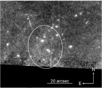
Figure 2: ESO/MPG 2.2m Wide Field Imager (WFI) I-band image of a possible galaxy cluster in the background of NGC 253. The white ellipse marks the source extent of the X-ray source as found in the source detection. The bottom quarter of the image is not covered by the WFI detector.

2.2 Images

We used all 4 observations to produce images. The observations have different pointing directions and position angles, so we obtained images where almost all the CCD gaps are filled. The single images, from the energy bands 1 to 5, were corrected for the detector background (electronic noise, high energy particles) by subtracting the surface brightness of the detector corners, that are outside of the field of view. The images were exposure and vignetting corrected, and adaptively smoothed with a Gaussian kernel, with sizes between 10″ and 47″ (Fig. 1). For a detailed description of this method see App. A. A false-colour image was produced by combining the images in the three lowest energy bands 1, 2, and 3, as channels red, green, and blue, respectively (Fig. 3). The image, after the point source removal is shown in Fig. 4.

Figure 3: Adaptively smoothed EPIC pn image of NGC 253. The colours correspond to the energy bands (0.2–0.5 keV, red), (0.5–1.0 keV, green) , and (1.0–2.0 keV, blue). Overplotted in white is the inclination corrected optical $D_{25}$ ellipse of NGC 253. The centre of the galaxy is marked with a black cross. Scale and orientation are indicated.

Figure 4: Adaptively smoothed EPIC pn image of the diffuse emission of NGC 253. Point-like sources have been removed. Overplotted in green are the regions that were used for extracting hardness ratios and spectra. The bright knot in the northwestern halo (see Sect. 3.2) is indicated by a blue circle. The inclination corrected optical $D_{25}$ ellipse is shown in white.

2.3 Hardness ratio maps and spectra

As a big advantage, compared to the observations by ROSAT and Chandra, the higher count rates in XMM-Newton allowed us to extract spectra with reasonable statistics from smaller regions in the disc and the halo. For the hardness ratios and spectra we again restricted ourselves to the EPIC pn data. We did not use observations 2 and 3 for hardness ratios and spectra, because after good time interval screening only little exposure was left (cf. Table 1).

Energy spectra of several regions (cf. Fig. 4) were extracted from the event files, using the SAS-task evselect, version 3.60, after removal of the point-like sources. To calculate the area of these regions, we used the task backscale, version 1.4.2. We produced background spectra using a region at the southwestern border of the FOV, together with observations where the filter wheel was closed. A detailed description of this procedure, which also handles the binning of the spectra, can be found in Appendix B. The final, background subtracted source spectrum for each region has a significance of at least 3 $\sigma$ in each data bin. The advantage of using this method is a more accurate background subtraction which also accounts for vignetting and the particle background. As shown in Appendix B, this can have a large effect (of up to $\sim$20%) on the flux values and it can eliminate the need of introducing a power law component to account for residuals at high energies in the spectral fits.

Since the emission is mostly confined to energies between 0.2 and 2.0 keV, we only calculated the hardness ratios HR1 and HR2, where HR1=(B₂-B₁)/(B₂+B₁), and HR2=(B₃-B₂)/(B₃+B₂). B₁, B₂, and B₃ are the count rates in the energy bands 1 to 3, i.e. 0.2–0.5 keV, 0.5–1.0 keV, and 1.0–2.0 keV, respectively. They were obtained by summing up the background subtracted counts in the spectra in the energy bands. Observations 1 and 4 were performed for EPIC pn using the medium and thin filter, respectively. As these filters have a significantly different throughput, we did not calculate the combined hardness ratios, but show the results for the two observations independently (Fig. 5 and Table 2). The errors on the hardness ratios were propagated from the errors on the counts in the spectra.

In order to fit the spectra with physical models, we created the proper response and anxiliary response files for extended sources for each spectrum. In XSPEC 11.3.2, we linked the model parameters between the two observations and included a global renormalisation factor to account for differences between the observations to fit the spectra from observations 1 and 4 simultaneously. To fit the spectra with physical models we used the chi-squared statistics in XSPEC. To assess the significance of additional model components, the Bayesian Information Criterion (BIC, introduced by Schwarz, 1978, an astronomical application can be found, e.g., in Liddle, 2004) was applied: a difference of 2 for the BIC is regarded as positive evidence, and of 6 or more as strong evidence, against the model with the larger value (Jeffreys, 1961; Mukherjee et al., 1998). We did not use the F-test, since this method is not valid to test if an additional absorption component is justified (Protassov et al., 2002), since the null value of the additional parameter is on the boundary of the set of possible parameter values, i.e. zero, and negative column density values are not supported by the tbabs (Wilms et al., 2000) model. For the BIC, these restrictions do not apply. The criteria for our best-fit models are the following: (i) the $\chi^{2}_{\nu}$ is below 1.4, (ii) the BIC difference between a given model and a model with more parameters is greater than 2, (iii) the errors on all model parameter are constrained, and (iv) the model is physically meaningful.

Figure 5: Hardness ratio maps of observations 1 (left) and 4 (right): The map was binned to the same regions as in Fig. 4. The higher the index, the harder the spectrum. The background colour corresponds to an artificially set value. We also show the inclination corrected optical $D_{25}$ ellipse. (top): HR1=(B₂-B₁)/(B₂+B₁), where B₁ and B₂ are the count rates in the energy bands 0.2–0.5 keV and 0.5–1.0 keV, respectively. (bottom): HR2=(B₃-B₂)/(B₃+B₂), where B₂ and B₃ are the count rates in the energy bands 0.5–1.0 keV and 1.0–2.0 keV, respectively.

Table 2: Comparison between hardness ratios, for the individual observations (obs 4: thin filter; obs 1: medium filter)

Region	HR1		HR2
	Obs 1	Obs 4	Obs 1	Obs 4
Northwestern halo
1	$0.16\pm 0.06$	$-0.04\pm 0.05$	$-0.44\pm 0.04$	$-0.46\pm 0.04$
2	$0.13\pm 0.06$	$-0.09\pm 0.05$	$-0.41\pm 0.04$	$-0.46\pm 0.05$
3	$0.18\pm 0.06$	$0.10\pm 0.04$	$-0.50\pm 0.04$	$-0.61\pm 0.03$
4	$0.26\pm 0.06$	$0.08\pm 0.05$	$-0.46\pm 0.04$	$-0.51\pm 0.04$
5	$0.05\pm 0.05$	$-0.06\pm 0.04$	$-0.56\pm 0.04$	$-0.58\pm 0.03$
6	$0.07\pm 0.04$	$0.05\pm 0.03$	$-0.52\pm 0.03$	$-0.65\pm 0.04$
7	$0.14\pm 0.05$	$0.12\pm 0.04$	$-0.54\pm 0.03$	$-0.59\pm 0.03$
2…4	$0.19\pm 0.03$	$0.04\pm 0.03$	$-0.46\pm 0.02$	$-0.54\pm 0.02$
5…7	$0.09\pm 0.03$	$0.05\pm 0.02$	$-0.53\pm 0.02$	$-0.62\pm 0.02$
1…7	$0.13\pm 0.02$	$0.03\pm 0.02$	$-0.50\pm 0.01$	$-0.58\pm 0.01$
Disc
8	$0.38\pm 0.07$	$0.39\pm 0.05$	$-0.23\pm 0.06$	$-0.25\pm 0.05$
9	$0.46\pm 0.06$	$0.42\pm 0.05$	$-0.31\pm 0.05$	$-0.30\pm 0.04$
10	$0.44\pm 0.08$	$0.60\pm 0.07$	$-0.18\pm 0.06$	$-0.14\pm 0.05$
11	$0.23\pm 0.05$	$0.10\pm 0.04$	$-0.48\pm 0.04$	$-0.54\pm 0.03$
12	$0.15\pm 0.06$	$-0.14\pm 0.05$	$-0.41\pm 0.04$	$-0.60\pm 0.04$
13	$0.43\pm 0.07$	$0.47\pm 0.05$	$-0.20\pm 0.06$	$-0.23\pm 0.04$
14	$0.30\pm 0.03$	$0.26\pm 0.02$	$-0.55\pm 0.03$	$-0.57\pm 0.02$
15	$0.01\pm 0.04$	$0.04\pm 0.03$	$-0.66\pm 0.03$	$-0.65\pm 0.03$
16	$0.45\pm 0.04$	$0.42\pm 0.03$	$-0.17\pm 0.04$	$-0.28\pm 0.03$
17	$0.31\pm 0.03$	$0.23\pm 0.02$	$-0.45\pm 0.03$	$-0.42\pm 0.02$
18	$0.17\pm 0.04$	$0.12\pm 0.03$	$-0.55\pm 0.03$	$-0.53\pm 0.03$
19	$0.37\pm 0.04$	$0.32\pm 0.03$	$-0.52\pm 0.03$	$-0.50\pm 0.03$
20	$0.27\pm 0.04$	$0.27\pm 0.03$	$-0.48\pm 0.03$	$-0.39\pm 0.03$
21	$0.21\pm 0.06$	$0.17\pm 0.05$	$-0.42\pm 0.04$	$-0.51\pm 0.03$
Southeastern halo
22	$-0.02\pm 0.06$	$-0.07\pm 0.05$	$-0.44\pm 0.04$	$-0.58\pm 0.04$
23	$0.02\pm 0.05$	$-0.11\pm 0.04$	$-0.50\pm 0.04$	$-0.55\pm 0.04$
24	$0.05\pm 0.08$	$-0.12\pm 0.07$	$-0.25\pm 0.05$	$-0.33\pm 0.06$
23+24	$0.03\pm 0.04$	$-0.12\pm 0.03$	$-0.41\pm 0.03$	$-0.48\pm 0.03$
25	$-0.14\pm 0.07$	$-0.21\pm 0.06$	$-0.26\pm 0.06$	$-0.44\pm 0.06$
22…24	$0.01\pm 0.03$	$-0.10\pm 0.03$	$-0.42\pm 0.02$	$-0.51\pm 0.03$
22…25	$-0.01\pm 0.03$	$-0.12\pm 0.02$	$-0.39\pm 0.02$	$-0.50\pm 0.02$

3 Results

To characterise the diffuse emission in the disc and the halo, we analysed images in different energy bands, and hardness ratios and spectra from several regions. The size of these regions was chosen to provide enough counts for a spectral analysis. As for the shape, in the disc the regions were chosen in a way that they follow the spiral arm structure. In the halo, we chose plane-parallel regions above the galactic disc. The projected heights of the halo regions are 2 kpc, with exception of the region furthest to the northwest (region 1), which has a projected height of 3 kpc. The regions are overplotted on top the false-colour X-ray image in Fig. 4. The hardness ratios in the different regions are given in Table 2 and shown graphically in Fig. 5.

3.1 Disc diffuse emission

The disc shows diffuse emission in energies up to $\sim$10 keV, where the harder emission is located close to the centre of NGC 253. The soft emission ($<$1 keV) shows the largest extent along the major axis. From the nucleus, it reaches $\sim$7.0 kpc to the northwest and $\sim$6.4 kpc to the southeast.

A prominent feature in the disc is the lack of very soft emission northwest of the major axis. This is already known from ROSAT observations (e.g. Pietsch et al., 2000) and can be explained by the geometry of the system: The galaxy’s disc is oriented so that we see the underside of the disc. The emission from the northwestern halo behind the disc is therefore absorbed by the intervening disc material.

The spectral properties in different regions of the disc are summarised in Table LABEL:tab:DiskFits. The spectra of all disc regions are shown in Fig. 6. A representative example (region 14) of one of these disc spectra shows lines from O VII ($\sim$0.57 keV), O VIII (0.65 keV), Fe XVII (0.73–0.83 keV), Ne IX ($\sim$0.91 keV), Ne X (1.0 keV), Mg XI ($\sim$1.3 keV), and Si XIII ($\sim$1.9 keV).

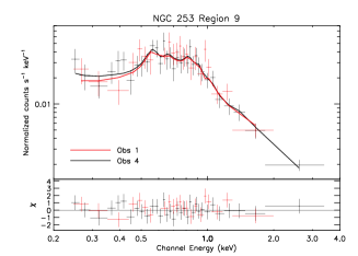
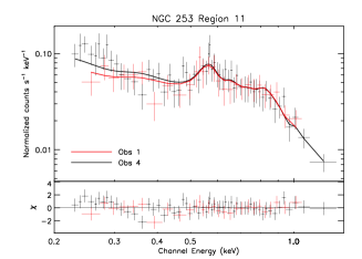
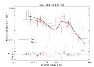
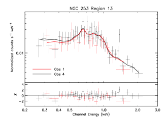
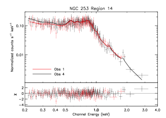
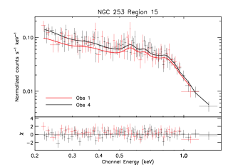
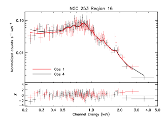
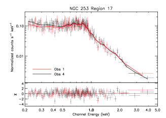
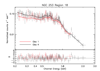
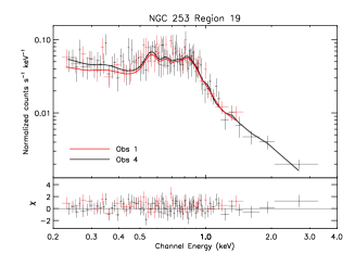
Figure 6: Spectra of different regions in the disc. The red and the black data points and model fits are from observations 1 and 4, respectively. The lower panel shows the residuals of the fits.

To fit the spectra, we tried several different models, which all contain an absorption model tbabs for the Galactic foreground $N_{\rm H}$ of $1.3\times 10^{20}$ cm^-2 (Dickey & Lockman, 1990). Also the abundances were fixed to solar values (see also Sec. 4.4) from Wilms et al. (2000). A simple one-temperature thin thermal plasma model (apec, Smith et al., 2001) did not result in a good fit (i.e. $\chi^{2}_{\nu}\leq 1.4$) in any case. Similarly, a power law model did not give good fits (see Table LABEL:tab:DiskFits). At least three components were necessary for most of the regions: two thin thermal plasmas plus a power law component. The power law was needed to account for the emission above $\sim$1 keV and probably results from point sources below the point source detection limit, or incomplete source removal due to too small extraction radii.

The obtained temperatures are quite uniform throughout the disc and vary from 0.1 to 0.3 keV and from 0.3 to 0.9 keV for the soft and the hard component, respectively. The intrinsic luminosity (corrected for Galactic absorption) of the diffuse emission within the inclination corrected optical $D_{25}$ ellipse is 2.4$\times 10^{39}$ erg s^-1 (0.2–10.0 keV), or 8.5$\times 10^{38}$ erg s^-1 (2.0–10 keV). Both values were corrected for the area of cut-out point-like sources.

The spectra decrease in hardness from the northwest to the southeast parallel to the minor axis, which can easily be seen in the hardness ratio maps (HR1, Fig. 5). This is not an effect caused by different temperatures, but by the increasing strength of the soft spectral component towards the southeast (compared to the hard component), as the optical depth through the halo on the near side of the disc increases.

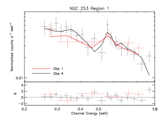
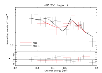
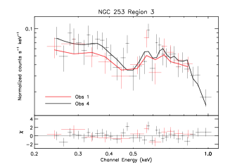
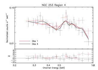
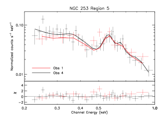
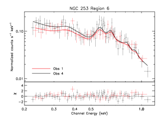
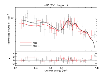
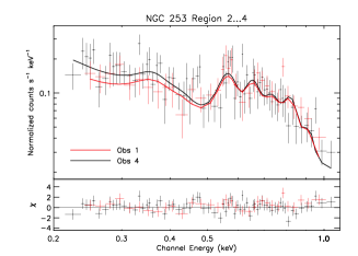
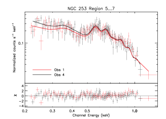
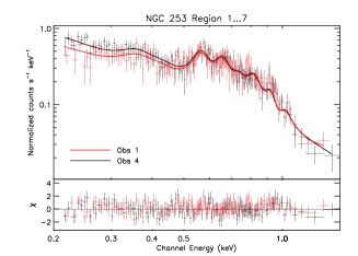
Figure 7: Spectra of regions in the northwestern halo (as Fig. 6).

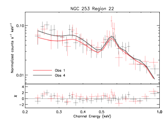
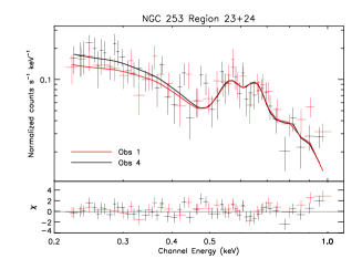
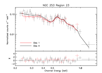
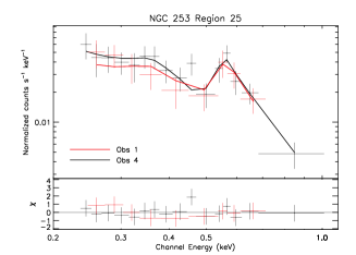
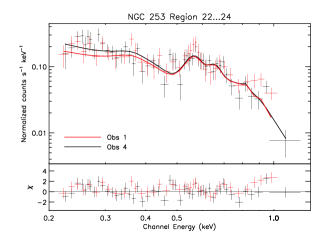
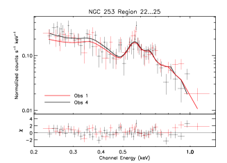
Figure 8: Spectra of different combined regions in the southeastern halo (as Fig. 6).

For the disc regions that lie in the absorption band (region 9) and along the nuclear outflow (regions 16, 17, and 18) we tested for additional absorption components. In other regions we do not expect a measurable absorber in the foreground with a sufficiently bright source in the background. In region 9, we obtain a column density of $0.50_{-0.17}^{+0.39}$$\times 10^{22}$ cm^-2 for the hard component. The region covering the northwestern outflow (region 16) closest to the centre shows values of $0.076_{-0.053}^{+0.086}$$\times 10^{22}$ cm^-2 and $0.58_{-0.18}^{+0.35}$$\times 10^{22}$ cm^-2 for the soft and hard component, respectively. Regions 17 and 18, covering the centre of NGC 253 and the southeastern outflow do not seem to require an additional absorption component.

In a few cases, the two thermal plasma plus a power law component model did not give the best fit. The southern region on the northeastern end of the disc (region 12) did not require a power law component. It does not cover a spiral arm of NGC 253, thus the contribution from point-like sources below the detection limit may not be significant. The region furthest to the south in the disc (region 21) was well fit with one thermal plasma and a power law. A second thermal plasma was not required.

We found that spectra are harder in regions which cover spiral arms. The northeastern regions of the disc (regions 11 & 12) are the best example for this. The region which covers the spiral arm (region 11) shows temperatures of $0.18^{+0.05}_{-0.04}$ and $0.58^{+0.16}_{-0.18}$ keV, whereas the region adjacent to the spiral arm (region 12) is significantly cooler with temperatures of $0.07\pm 0.01$ and $0.25^{+0.04}_{-0.03}$ keV. The latter spectrum is actually more similar to the typical halo spectrum (see next section).

3.2 Halo diffuse emission

The halo shows emission only below $\sim$1 keV. Its projected maximum extent is $\sim$9.0 kpc to the northwest, and $\sim$6.3 kpc to the southeast, perpendicular to the major axis. The general shape resembles a horn structure. This was already seen with ROSAT (e.g. Pietsch et al., 2000), and Chandra (e.g. Strickland et al., 2002, using the term ”X-shaped morphology”). In the northwestern halo, the EPIC pn images only show the eastern horn. In the southeastern halo, both the eastern and the western horn are visible in the energies between 0.2 and 0.5 keV. At higher energies, the western horn is not visible.

On smaller scales the halo emission seems not to be uniformly distributed. It shows a patchy structure, as was seen before in the ROSAT data. One notable feature is a brighter knot (see Fig. 4), which coincides with the nuclear outflow axis in the northwestern halo at a height of about 3.5 kpc above the disc. It is bright in energies between 0.2 and 1.0 keV and appears yellow in the false-colour image (Fig. 3). We checked whether any of the detected structures coincide with chip gaps of the detector, and could therefore be artificial, but no correlation was found.

The spectral properties in different regions in the halo are summarised in Table LABEL:tab:HaloFits. To fit the spectra, we applied the same approach as for the disc. Again, simple models cannot describe the spectra. A model with two thin thermal plasmas gave a good fit in all regions in the halo. In region 6, and all regions containing region 6, adding a power law component results in a better fit, possibly pointing at a cosmic ray contribution.

The southeastern halo is softer than the northwestern halo, which results in redder colours in the southeastern halo in the EPIC pn false-colour image (Fig. 3), and also in lower values in HR1. A fit to the spectrum of the whole northwestern halo gave temperatures of $0.10\pm 0.01$ and $0.31\pm 0.02$ keV. The spectrum in the southeastern halo is similar, with temperatures of $0.09\pm 0.02$ and $0.29^{+0.03}_{-0.04}$ keV. The difference in hardness is because the two plasma components contribute different amounts. Compared to the normalisation of the hotter plasma, the normalisation of the cooler plasma is about 2.1 times stronger in the southeastern halo, with respect to the northwestern halo.

The good statistics of the EPIC pn data allowed a further subdivision of the halo into smaller regions. The spectra of all halo regions are shown in Figs. 7 and 8. A representative example (region 7) of one of these halo spectra shows prominent oxygen lines at 0.57 keV (O VII) and 0.65 keV (O VIII) and also an iron line at $\sim$0.8 keV (Fe XVII).

The halo is not uniform in its spectral properties on smaller scales. The northwestern halo is softer in the east than in the west, while the southeastern halo is softer further away from the disc (see HR1 maps in Fig. 5). Additionally, there is a marginal indication of a hardening of the emission along the direction of the northwestern outflow (regions 3 and 6, significance: 1.0–1.6$\,\sigma$ in HR1 and 0.40–0.80$\,\sigma$ in HR2).

The total intrinsic luminosity for the diffuse emission, corrected for the area of the removed point-like sources, in the northwestern halo is 8.4$\times 10^{38}$ erg s^-1 (0.2–1.5 keV), compared to 2.3$\times 10^{38}$ erg s^-1 in the southeastern halo. To calculate electron densities, we assumed a volume for the emitting region. We modeled the northwestern halo with a cylinder with a radius of 4.3 kpc and a height of 4.2 kpc, plus a cylindrical segment with a height of 4.2 kpc, a radius of 4.3 kpc and a width in the southeast-northwest direction of 3.0 kpc (to model region 1). This gives a volume of 298 kpc³ or $8.7\times 10^{66}$ cm³. For the southeastern halo we assumed a cylinder with a radius of 3.5 kpc and a height of 2.0 kpc, plus a cylindrical segment with a height of 2.0 kpc, a radius of 3.5 kpc and a width in the southeast-northwest direction of 3.0 kpc (region 25), resulting in a volume of 113 kpc³ or $3.3\times 10^{66}$ cm³. To calculate densities and the total mass in the emission regions, we corrected the volumes for the cut-out point-like sources. Using the emission measure of the fit (cf. the documentation of the apec model in XSPEC), the resulting densities are $3.2\,\eta^{-0.5}\times 10^{-3}$ cm^-3 and $4.7\,\eta^{-0.5}\times 10^{-3}$ cm^-3 for the northwestern and southeastern halo, respectively. $\eta$ is the volume filling factor ($\eta\leq 1$). With solar abundances from Wilms et al. (2000), this implies total masses of $3.3\,\eta^{-0.5}\times 10^{7}$ M_☉ and $1.8\,\eta^{-0.5}\times 10^{7}$ M_☉ for the northwestern and southeastern halo, respectively.

Table 3: Spectral fits to the disk regions.

Region/model	$\chi^{2}_{\nu}\,(\chi^{2}/\nu)$	BIC	$N_{\rm H}$	kT	norm	$N_{\rm H}$	kT	norm	$\Gamma$	norm
			($10^{22}$ cm-2)	(keV)	($10^{-5}$)	($10^{22}$ cm-2)	(kev)	($10^{-5}$)		($10^{-5}$)
Region 9
po	2.8 (143.4/52)	60.7	$\dots$	$\dots$	$\dots$	$\dots$	$\dots$	$\dots$	$1.7_{-0.1}^{+0.1}$	$1.8_{-0.2}^{+0.2}$
apec	4.5 (232.9/52)	86.9	$\dots$	$0.37_{-0.03}^{+0.03}$	$1.1_{-0.2}^{+0.2}\times 10^{5}$	$\dots$	$\dots$	$\dots$	$\dots$	$\dots$
apec+po	1.2 (60.3/50)	21.9	$\dots$	$0.36_{-0.06}^{+0.09}$	$1.8_{-0.7}^{+0.7}$	$\dots$	$\dots$	$\dots$	$1.3_{-0.3}^{+0.3}$	$1.1_{-0.3}^{+0.3}$
apec+apec	1.2 (58.9/51)	19.8	$\dots$	$0.37_{-0.07}^{+0.14}$	$1.6_{-0.6}^{+0.5}$	$\dots$	$7.74_{-5.27}^{+\mbox{n.c.}^{1}}$	$4.9_{-1.2}^{+1.4}$	$\dots$	$\dots$
apec+apec+po	0.9 (44.3/48)	13.2	$\dots$	$0.24_{-0.09}^{+0.09}$	$1.2_{-0.8}^{+1.2}$	$\dots$	$0.72_{-0.21}^{+0.28}$	$1.1_{-0.9}^{+0.6}$	$0.96_{-0.34}^{+0.44}$	$0.81_{-0.49}^{+0.43}$
apec+tbabs(apec)+po	0.8 (36.4/47)	6.6	$\dots$	$0.17_{-0.07}^{+0.08}$	$1.1_{-0.9}^{+1.2}$	$0.50_{-0.17}^{+0.39}$	$0.32_{-0.07}^{+0.08}$	$9.2_{-4.9}^{+4.7}$	$1.1_{-0.4}^{+0.5}$	$0.87_{-0.59}^{+0.44}$
tbabs(apec)+apec+po	no convergence towards a solution where the cooler component is absorbed
tbabs(apec)+tbabs(apec)+po	0.7 (33.2/46)	5.6	$0.60_{-0.16}^{+1.04}$	$0.14_{-0.04}^{+0.03}$	$70_{-70}^{+76}$	$0.46_{-0.23}^{+0.34}$	$0.39_{-0.12}^{+0.27}$	$3.9_{-2.2}^{+2.2}$	$1.5_{-0.5}^{+0.5}$	$1.1_{-0.4}^{+0.4}$
Region 11
po	1.6 (130.8/82)	46.1	$\dots$	$\dots$	$\dots$	$\dots$	$\dots$	$\dots$	$2.2_{-0.2}^{+0.2}$	$3.6_{-0.4}^{+0.4}$
apec	2.1 (171.2/82)	68.7	$\dots$	$0.28_{-0.04}^{+0.01}$	$0.90_{-0.12}^{+0.14}\times 10^{5}$	$\dots$	$\dots$	$\dots$	$\dots$	$\dots$
apec+po	0.9 (73.4/80)	6.4	$\dots$	$0.29_{-0.06}^{+0.07}$	$2.9_{-0.9}^{+2.3}$	$\dots$	$\dots$	$\dots$	$2.4_{-0.7}^{+0.3}$	$2.4_{-1.3}^{+0.4}$
apec+apec	0.9 (68.2/80)	0.2	$\dots$	$0.14_{-0.02}^{+0.03}$	$7.1_{-1.5}^{+2.2}$	$\dots$	$0.59_{-0.15}^{+0.08}$	$3.1_{-0.6}^{+0.5}$	$\dots$	$\dots$
apec+apec+po	0.6 (47.0/78)	-22.2	$\dots$	$0.18_{-0.04}^{+0.05}$	$3.4_{-1.3}^{+1.4}$	$\dots$	$0.58_{-0.18}^{+0.16}$	$1.9_{-0.8}^{+0.8}$	$2.5_{-0.8}^{+0.5}$	$1.2_{-1.2}^{+0.8}$
Region 12
po	2.0 (68.5/34)	30.3	$\dots$	$\dots$	$\dots$	$\dots$	$\dots$	$\dots$	$2.4_{-0.3}^{+0.3}$	$1.7_{-0.4}^{+0.4}$
apec	2.5 (85.4/34)	38.3	$\dots$	$0.23_{-0.02}^{+0.02}$	$1.1_{-0.2}^{+0.2}\times 10^{5}$	$\dots$	$\dots$	$\dots$	$\dots$	$\dots$
apec+po	1.4 (43.9/32)	21.5	$\dots$	$0.24_{-0.03}^{+0.03}$	$2.6_{-0.6}^{+0.7}$	$\dots$	$\dots$	$\dots$	$4.8_{-0.6}^{+0.4}$	$0.090_{-0.083}^{+0.075}$
apec+apec	1.4 (43.3/32)	21.0	$\dots$	$0.07_{-0.01}^{+0.01}$	$17_{-10}^{+12}$	$\dots$	$0.25_{-0.03}^{+0.04}$	$2.7_{-0.6}^{+0.6}$	$\dots$	$\dots$
apec+apec+po	1.2 (37.1/30)	22.6	$\dots$	$0.07_{-0.01}^{+0.02}$	$17_{-13}^{+30}$	$\dots$	$0.22_{-0.07}^{+0.05}$	$2.1_{-1.2}^{+0.9}$	$-1.1_{-\mbox{n.c.}^{1}}^{+3.6}$	$1.4_{-1.4}^{+1.3}$
Region 13
po	1.8 (103.6/58)	41.0	$\dots$	$\dots$	$\dots$	$\dots$	$\dots$	$\dots$	$1.5_{-0.1}^{+0.1}$	$1.9_{-0.2}^{+0.2}$
apec	4.0 (234.7/58)	90.0	$\dots$	$0.37_{-0.03}^{+0.04}$	$0.81_{-0.16}^{+0.17}\times 10^{5}$	$\dots$	$\dots$	$\dots$	$\dots$	$\dots$
apec+po	0.9 (52.3/56)	8.1	$\dots$	$0.34_{-0.05}^{+0.08}$	$1.6_{-0.7}^{+0.7}$	$\dots$	$\dots$	$\dots$	$0.93_{-0.35}^{+0.33}$	$1.2_{-0.3}^{+0.4}$
apec+apec	1.0 (53.9/56)	9.9	$\dots$	$0.36_{-0.07}^{+0.31}$	$1.3_{-0.5}^{+0.5}$	$\dots$	$64_{-59}^{+\mbox{n.c.}^{1}}$	$8.9_{-2.2}^{+2.1}$	$\dots$	$\dots$
apec+apec+po	0.8 (41.3/54)	2.2	$\dots$	$0.30_{-0.06}^{+0.09}$	$1.5_{-1.1}^{+0.8}$	$\dots$	$0.87_{-0.29}^{+\mbox{n.c.}^{1}}$	$0.67_{-0.63}^{+0.70}$	$0.66_{-0.50}^{+0.52}$	$0.94_{-0.60}^{+0.46}$
Region 14
po	2.9 (803.9/279)	306.6	$\dots$	$\dots$	$\dots$	$\dots$	$\dots$	$\dots$	$2.3_{-0.1}^{+0.1}$	$5.4_{-0.3}^{+0.3}$
apec	2.2 (619.4/279)	233.4	$\dots$	$0.34_{-0.01}^{+0.02}$	$0.91_{-0.07}^{+0.07}\times 10^{5}$	$\dots$	$\dots$	$\dots$	$\dots$	$\dots$
apec+po	0.8 (217.4/277)	-49.6	$\dots$	$0.38_{-0.04}^{+0.09}$	$8.1_{-1.7}^{+1.6}$	$\dots$	$\dots$	$\dots$	$2.2_{-0.2}^{+0.3}$	$3.3_{-1.0}^{+0.4}$
apec+apec	1.0 (286.8/277)	28.3	$\dots$	$0.14_{-0.01}^{+0.02}$	$8.8_{-1.5}^{+2.2}$	$\dots$	$0.61_{-0.03}^{+0.03}$	$8.4_{-0.7}^{+0.7}$	$\dots$	$\dots$
apec+apec+po	0.5 (149.0/275)	-144.4	$\dots$	$0.20_{-0.05}^{+0.05}$	$4.3_{-1.6}^{+1.0}$	$\dots$	$0.59_{-0.05}^{+0.06}$	$5.7_{-1.6}^{+1.1}$	$2.1_{-0.3}^{+0.2}$	$2.2_{-0.5}^{+0.6}$
Region 15
po	1.5 (182.4/120)	58.7	$\dots$	$\dots$	$\dots$	$\dots$	$\dots$	$\dots$	$2.6_{-0.1}^{+0.1}$	$2.9_{-0.3}^{+0.3}$
apec	2.6 (310.1/120)	123.4	$\dots$	$0.26_{-0.01}^{+0.01}$	$1.0_{-0.1}^{+0.1}\times 10^{5}$	$\dots$	$\dots$	$\dots$	$\dots$	$\dots$
apec+po	0.8 (90.4/118)	-17.4	$\dots$	$0.30_{-0.04}^{+0.04}$	$3.4_{-1.0}^{+1.0}$	$\dots$	$\dots$	$\dots$	$2.9_{-0.3}^{+0.2}$	$1.5_{-0.4}^{+0.4}$
apec+apec	1.0 (112.8/118)	9.7	$\dots$	$0.10_{-0.01}^{+0.01}$	$13_{-3}^{+4}$	$\dots$	$0.37_{-0.04}^{+0.04}$	$4.4_{-1.0}^{+0.9}$	$\dots$	$\dots$
apec+apec+po	0.7 (80.2/116)	-22.4	$\dots$	$0.20_{-0.06}^{+0.05}$	$2.8_{-1.3}^{+0.9}$	$\dots$	$0.59_{-0.15}^{+0.15}$	$1.6_{-1.4}^{+0.9}$	$3.1_{-0.3}^{+0.3}$	$1.0_{-0.4}^{+0.5}$
Region 16 (NW outflow)
po	2.7 (415.1/155)	162.8	$\dots$	$\dots$	$\dots$	$\dots$	$\dots$	$\dots$	$1.6_{-0.1}^{+0.1}$	$3.5_{-0.2}^{+0.2}$
apec	5.7 (878.7/155)	280.5	$\dots$	$0.41_{-0.02}^{+\mbox{n.c.}^{1}}$	$1.0_{-0.1}^{+0.1}\times 10^{5}$	$\dots$	$\dots$	$\dots$	$\dots$	$\dots$
apec+po	1.1 (161.5/153)	24.7	$\dots$	$0.64_{-0.06}^{+0.09}$	$2.7_{-0.5}^{+0.5}$	$\dots$	$\dots$	$\dots$	$1.4_{-0.1}^{+0.1}$	$2.5_{-0.3}^{+0.3}$
apec+apec	0.9 (145.2/153)	8.0	$\dots$	$0.63_{-0.08}^{+0.09}$	$2.4_{-0.4}^{+0.6}$	$\dots$	$\dots$	$\dots$	$5.9_{-2.2}^{+5.6}$	$10_{-2}^{+1}$
apec+apec+po	1.0 (153.9/151)	27.2	$\dots$	$0.22_{-0.22}^{+0.24}$	$0.65_{-0.65}^{+2.64}$	$\dots$	$0.66_{-0.08}^{+0.13}$	$2.7_{-1.1}^{+0.6}$	$1.3_{-0.1}^{+0.1}$	$2.2_{-0.4}^{+0.4}$
tbabs(apec)+apec+po	1.0 (145.8/150)	23.8	$2.6_{-0.8}^{+2.7}$	$0.50_{-0.20}^{+0.16}$	$35_{-22}^{+16}$	$\dots$	$0.61_{-0.18}^{+0.08}$	$2.8_{-0.5}^{+0.5}$	$1.5_{-0.2}^{+0.2}$	$2.1_{-0.4}^{+0.4}$
apec+tbabs(apec)+po	0.8 (126.1/150)	1.0	$\dots$	$0.25_{-0.07}^{+0.08}$	$1.8_{-1.0}^{+2.1}$	$0.54_{-0.18}^{+0.24}$	$0.59_{-0.12}^{+0.11}$	$9.1_{-5.2}^{+3.7}$	$1.4_{-0.2}^{+0.2}$	$2.0_{-0.5}^{+0.4}$
tbabs(apec)+tbabs(apec)+po	0.8 (119.9/149)	-1.9	$0.076_{-0.053}^{+0.086}$	$0.23_{-0.08}^{+0.08}$	$2.7_{-0.1}^{+2.2}$	$0.58_{-0.18}^{+0.35}$	$0.58_{-0.41}^{+0.11}$	$9.5_{-4.7}^{+3.4}$	$1.5_{-0.2}^{+0.2}$	$2.2_{-0.4}^{+0.5}$
Region 17 (Centre)
po	2.1 (534.4/253)	199.8	$\dots$	$\dots$	$\dots$	$\dots$	$\dots$	$\dots$	$2.0_{-0.1}^{+0.1}$	$5.1_{-0.2}^{+0.2}$
apec	4.2 (1064.0/253)	375.4	$\dots$	$0.34_{-0.01}^{+0.03}$	$1.0_{-0.1}^{+0.1}\times 10^{5}$	$\dots$	$\dots$	$\dots$	$\dots$	$\dots$
apec+po	0.8 (199.3/251)	-40.7	$\dots$	$0.37_{-0.03}^{+0.04}$	$5.0_{-0.8}^{+1.1}$	$\dots$	$\dots$	$\dots$	$1.8_{-0.1}^{+0.1}$	$3.5_{-0.4}^{+0.3}$
apec+apec	2.9 (741.0/252)	294.3	$\dots$	$0.13_{-0.01}^{+0.01}$	$7.6_{-1.7}^{+1.7}$	$\dots$	$0.63_{-0.03}^{+0.03}$	$6.5_{-0.5}^{+0.5}$	$\dots$	$\dots$
apec+apec+po	0.8 (187.1/249)	-45.7	$\dots$	$0.24_{-0.04}^{+0.06}$	$2.6_{-1.4}^{+1.6}$	$\dots$	$0.58_{-0.12}^{+0.08}$	$2.8_{-1.1}^{+1.2}$	$1.7_{-0.1}^{+0.2}$	$3.3_{-0.6}^{+0.5}$
tbabs(apec)+apec+po	0.8 (186.4/248)	-41.1	$<0.21$	$0.24_{-0.06}^{+0.05}$	$2.6_{-1.5}^{+1.6}$	$\dots$	$0.58_{-0.14}^{+0.09}$	$2.9_{-1.4}^{+1.2}$	$1.7_{-0.1}^{+0.2}$	$3.2_{-0.5}^{+0.6}$
apec+tbabs(apec)+po	0.8 (186.4/248)	-41.1	$\dots$	$0.24_{-0.06}^{+0.05}$	$2.6_{-1.5}^{+1.6}$	$<0.21$	$0.58_{-0.13}^{+0.09}$	$2.9_{-0.8}^{+1.2}$	$1.7_{-0.1}^{+0.2}$	$3.2_{-0.5}^{+0.6}$
tbabs(apec)+tbabs(apec)+po	0.8 (186.4/247)	-35.6	$<0.22$	$0.24_{-0.07}^{+0.06}$	$2.6_{-1.6}^{+1.7}$	$<0.19$	$0.58_{-0.14}^{+0.09}$	$2.9_{-1.6}^{+1.3}$	$1.7_{-0.1}^{+0.2}$	$3.2_{-0.6}^{+0.7}$
Region 18 (SE outflow)
po	1.5 (227.8/156)	67.9	$\dots$	$\dots$	$\dots$	$\dots$	$\dots$	$\dots$	$2.3_{-0.1}^{+0.1}$	$3.2_{-0.2}^{+0.2}$
apec	2.2 (336.8/156)	129.7	$\dots$	$0.29_{-0.01}^{+0.01}$	$1.1_{-0.1}^{+0.1}\times 10^{5}$	$\dots$	$\dots$	$\dots$	$\dots$	$\dots$
apec+po	0.6 (93.6/154)	-62.5	$\dots$	$0.29_{-0.03}^{+0.03}$	$3.8_{-1.1}^{+0.7}$	$\dots$	$\dots$	$\dots$	$2.2_{-0.3}^{+0.3}$	$2.0_{-0.3}^{+0.5}$
apec+apec	1.3 (203.4/154)	60.2	$\dots$	$0.19_{-0.06}^{+0.02}$	$5.3_{-0.7}^{+0.6}$	$\dots$	$0.72_{-0.11}^{+12.75}$	$2.8_{-0.5}^{+0.5}$	$\dots$	$\dots$
apec+apec+po	0.5 (82.1/152)	-73.1	$\dots$	$0.24_{-0.04}^{+0.04}$	$2.9_{-1.3}^{+1.2}$	$\dots$	$0.66_{-0.22}^{+0.19}$	$1.2_{-0.8}^{+1.0}$	$2.3_{-0.3}^{+0.3}$	$1.8_{-0.5}^{+0.5}$
tbabs(apec)+apec+po	0.5 (82.1/151)	-68.0	$<0.16$	$0.24_{-0.04}^{+0.05}$	$2.9_{-1.4}^{+1.5}$	$\dots$	$0.66_{-0.55}^{+0.20}$	$1.2_{-1.2}^{+1.1}$	$2.3_{-0.4}^{+0.3}$	$1.8_{-0.5}^{+0.6}$
apec+tbabs(apec)+po	0.5 (82.1/151)	-68.0	$\dots$	$0.24_{-0.04}^{+0.06}$	$2.9_{-1.3}^{+1.4}$	$<54$	$0.66_{-0.51}^{+0.25}$	$1.2_{-1.2}^{+1.4}$	$2.3_{-0.4}^{+0.3}$	$1.8_{-0.6}^{+0.6}$
tbabs(apec)+tbabs(apec)+po	0.5 (82.1/150)	-62.9	$<0.17$	$0.24_{-0.05}^{+0.06}$	$2.9_{-1.4}^{+1.6}$	$0.0_{-0.0}^{+\mbox{n.c.}^{1}}$	$0.66_{-\mbox{n.c.}^{1}}^{+0.30}$	$1.2_{-1.2}^{+1.5}$	$2.3_{-0.3}^{+0.3}$	$1.8_{-0.6}^{+0.6}$
Region 19
po	2.5 (295.9/118)	117.9	$\dots$	$\dots$	$\dots$	$\dots$	$\dots$	$\dots$	$2.0_{-0.1}^{+0.1}$	$2.9_{-0.2}^{+0.2}$
apec	2.5 (297.0/118)	118.3	$\dots$	$0.33_{-0.01}^{+0.02}$	$1.1_{-0.1}^{+0.1}\times 10^{5}$	$\dots$	$\dots$	$\dots$	$\dots$	$\dots$
apec+po	1.0 (114.3/116)	13.3	$\dots$	$0.33_{-0.03}^{+0.06}$	$3.9_{-1.1}^{+1.0}$	$\dots$	$\dots$	$\dots$	$1.6_{-0.3}^{+0.4}$	$1.8_{-0.6}^{+0.3}$
apec+apec	1.5 (176.3/116)	65.3	$\dots$	$0.18_{-0.04}^{+0.04}$	$3.4_{-0.9}^{+0.5}$	$\dots$	$0.64_{-0.05}^{+0.10}$	$3.4_{-0.6}^{+0.6}$	$\dots$	$\dots$
apec+apec+po	0.7 (84.5/114)	-13.4	$\dots$	$0.19_{-0.05}^{+0.05}$	$2.7_{-1.0}^{+0.8}$	$\dots$	$0.59_{-0.11}^{+0.10}$	$2.4_{-0.9}^{+0.8}$	$1.1_{-0.3}^{+0.6}$	$1.1_{-0.8}^{+0.5}$
Region 20
po	2.4 (198.2/81)	81.1	$\dots$	$\dots$	$\dots$	$\dots$	$\dots$	$\dots$	$2.0_{-0.1}^{+0.1}$	$4.0_{-0.3}^{+0.3}$
apec	3.7 (300.1/81)	115.5	$\dots$	$0.31_{-0.01}^{+0.01}$	$1.1_{-0.1}^{+0.1}\times 10^{5}$	$\dots$	$\dots$	$\dots$	$\dots$	$\dots$
apec+po	1.1 (83.0/79)	17.7	$\dots$	$0.30_{-0.03}^{+0.03}$	$4.0_{-1.1}^{+1.0}$	$\dots$	$\dots$	$\dots$	$1.7_{-0.2}^{+0.3}$	$2.5_{-0.5}^{+0.6}$
apec+apec	2.6 (205.9/79)	93.1	$\dots$	$0.18_{-0.04}^{+0.03}$	$4.0_{-0.5}^{+1.6}$	$\dots$	$0.64_{-0.08}^{+85.12}$	$3.7_{-2.1}^{+0.5}$	$\dots$	$\dots$
apec+apec+po	1.0 (73.7/77)	16.6	$\dots$	$0.21_{-0.05}^{+0.05}$	$3.0_{-1.8}^{+1.1}$	$\dots$	$0.57_{-0.47}^{+0.16}$	$1.7_{-1.6}^{+0.8}$	$1.5_{-0.3}^{+0.4}$	$2.2_{-0.7}^{+0.7}$
Region 21
po	1.2 (48.8/41)	13.0	$\dots$	$\dots$	$\dots$	$\dots$	$\dots$	$\dots$	$1.7_{-0.2}^{+0.2}$	$2.8_{-0.4}^{+0.5}$
apec	2.1 (87.7/41)	38.2	$\dots$	$0.26_{-0.01}^{+0.03}$	$1.1_{-0.2}^{+0.2}\times 10^{5}$	$\dots$	$\dots$	$\dots$	$\dots$	$\dots$
apec+po	0.8 (32.3/39)	2.7	$\dots$	$0.20_{-0.07}^{+0.07}$	$1.7_{-1.1}^{+0.7}$	$\dots$	$\dots$	$\dots$	$1.4_{-0.8}^{+0.6}$	$2.1_{-0.7}^{+0.8}$
apec+apec	1.1 (43.2/39)	15.2	$\dots$	$0.16_{-0.03}^{+0.06}$	$3.3_{-0.8}^{+1.0}$	$\dots$	$0.63_{-0.18}^{+0.14}$	$1.6_{-0.4}^{+0.4}$	$\dots$	$\dots$
apec+apec+po	0.8 (30.2/37)	7.4	$\dots$	$0.18_{-0.18}^{+0.08}$	$1.6_{-1.6}^{+1.1}$	$\dots$	$0.58_{-\mbox{n.c.}^{1}}^{+\mbox{n.c.}^{1}}$	$0.45_{-0.45}^{+0.65}$	$1.5_{-1.2}^{+0.7}$	$1.7_{-1.2}^{+1.2}$
1n.c.: not constrained.
NOTE: All errors are 90% confidence for a number of interesting parameters equal to the number of free parameters in the model (2, 4, 6, 7, 8, or 9 free parameters depending on the model). Thin thermal plasma models are apec, absorption models are tbabs. All models have a fixed foreground absorption of $1.3\times 10^{20}$ cm-2. The preferred model is printed in bold font.

Table 4: Spectral fits to the northwestern halo regions.

Region/model	$\chi^{2}_{\nu}\,(\chi^{2}/\nu)$	BIC	kT	norm	kT	norm	$\Gamma$	norm
			(keV)	($10^{-5}$)	(kev)	($10^{-5}$)		($10^{-5}$)
Northwestern halo
Region 1
po	1.1 (25.9/23)	7.3	$\dots$	$\dots$	$\dots$	$\dots$	$2.0_{-0.3}^{+0.3}$	$6.1_{-1.3}^{+1.4}$
apec	3.9 (88.6/23)	38.1	$0.25_{-0.02}^{+0.02}$	$1.1_{-0.2}^{+0.3}\times 10^{5}$	$\dots$	$\dots$	$\dots$	$\dots$
apec+po	1.1 (22.1/21)	9.8	$0.19_{-0.19}^{+0.21}$	$1.3_{-1.3}^{+2.9}$	$\dots$	$\dots$	$1.9_{-0.6}^{+0.6}$	$5.6_{-2.0}^{+1.8}$
apec+apec	1.0 (21.1/21)	8.6	$0.10_{-0.02}^{+0.02}$	$19_{-8.3}^{+8.5}$	$0.35_{-0.05}^{+0.06}$	$5.6_{-1.5}^{+1.6}$	$\dots$	$\dots$
apec+apec+po	0.9 (16.3/19)	8.6	$0.09_{-0.07}^{+0.02}$	$20_{-20}^{+21}$	$0.29_{-0.29}^{+0.20}$	$2.6_{-2.6}^{+3.1}$	$0.55_{-\mbox{n.c.}^{1}}^{+1.75}$	$5.3_{-3.6}^{+4.0}$
Region 2
po	1.1 (21.7/20)	5.9	$\dots$	$\dots$	$\dots$	$\dots$	$2.0_{-0.4}^{+0.4}$	$3.1_{-0.8}^{+0.9}$
apec	2.6 (51.4/20)	24.9	$0.24_{-0.02}^{+0.02}$	$1.1_{-0.2}^{+0.3}\times 10^{5}$	$\dots$	$\dots$	$\dots$	$\dots$
apec+po	0.7 (12.5/18)	-0.1	$0.24_{-0.06}^{+0.08}$	$2.0_{-1.4}^{+1.5}$	$\dots$	$\dots$	$2.5_{-0.9}^{+0.6}$	$1.5_{-1.0}^{+0.9}$
apec+apec	0.8 (14.6/18)	3.3	$0.10_{-0.02}^{+0.03}$	$8.3_{-3.8}^{+4.2}$	$0.32_{-0.05}^{+0.06}$	$3.0_{-0.9}^{+1.0}$	$\dots$	$\dots$
apec+apec+po	0.7 (11.8/16)	4.8	$0.16_{-0.16}^{+\mbox{n.c.}^{1}}$	$1.4_{-1.4}^{+2.5}$	$0.31_{-0.31}^{+\mbox{n.c.}^{1}}$	$1.7_{-1.7}^{+2.1}$	$2.9_{-1.3}^{+0.9}$	$0.84_{-0.84}^{+0.84}$
Region 3
po	1.6 (67.0/41)	26.6	$\dots$	$\dots$	$\dots$	$\dots$	$1.7_{-0.3}^{+0.3}$	$4.5_{-0.7}^{+0.8}$
apec	2.4 (97.9/41)	42.9	$0.29_{-0.02}^{+0.02}$	$1.1_{-0.2}^{+0.2}\times 10^{5}$	$\dots$	$\dots$	$\dots$	$\dots$
apec+po	1.1 (41.2/39)	13.2	$0.32_{-0.04}^{+0.06}$	$3.8_{-1.1}^{+1.4}$	$\dots$	$\dots$	$3.1_{-0.6}^{+0.3}$	$0.87_{-0.66}^{+0.54}$
apec+apec	0.9 (35.3/39)	6.6	$0.09_{-0.02}^{+0.01}$	$12_{-5}^{+6}$	$0.34_{-0.03}^{+0.05}$	$4.6_{-0.9}^{+0.9}$	$\dots$	$\dots$
apec+apec+po	0.9 (34.0/37)	12.5	$0.09_{-0.02}^{+0.02}$	$12_{-6}^{+9}$	$0.33_{-0.05}^{+0.07}$	$4.2_{-1.6}^{+1.3}$	$-0.11_{-\mbox{n.c.}^{1}}^{+2.77}$	$1.0_{-1.0}^{+2.1}$
Region 4
po	1.7 (45.1/27)	19.5	$\dots$	$\dots$	$\dots$	$\dots$	$1.8_{-0.3}^{+0.3}$	$3.2_{-0.6}^{+0.7}$
apec	1.8 (47.8/27)	21.2	$0.26_{-0.02}^{+0.02}$	$1.2_{-0.2}^{+0.3}\times 10^{5}$	$\dots$	$\dots$	$\dots$	$\dots$
apec+po	1.0 (24.4/25)	8.5	$0.29_{-0.05}^{+0.05}$	$3.1_{-1.3}^{+1.3}$	$\dots$	$\dots$	$2.9_{-1.1}^{+0.6}$	$0.71_{-0.68}^{+0.59}$
apec+apec	0.7 (16.5/25)	-2.9	$0.11_{-0.03}^{+0.04}$	$5.7_{-2.9}^{+3.9}$	$0.33_{-0.04}^{+0.07}$	$3.3_{-0.9}^{+0.9}$	$\dots$	$\dots$
apec+apec+po	0.7 (16.4/23)	3.7	$0.11_{-0.04}^{+0.08}$	$5.6_{-4.7}^{+4.0}$	$0.34_{-0.05}^{+0.09}$	$3.2_{-1.2}^{+1.4}$	$-0.96_{-\mbox{n.c.}^{1}}^{+\mbox{n.c.}^{1}}$	$0.0_{-0.0}^{+2.8}$
Region 5
po	1.5 (63.3/43)	23.0	$\dots$	$\dots$	$\dots$	$\dots$	$2.3_{-0.2}^{+0.2}$	$2.8_{-0.5}^{+0.5}$
apec	2.5 (109.3/43)	47.5	$0.23_{-0.03}^{+0.01}$	$1.1_{-0.2}^{+0.2}\times 10^{5}$	$\dots$	$\dots$	$\dots$	$\dots$
apec+po	0.8 (32.9/41)	1.1	$0.21_{-0.04}^{+0.04}$	$2.5_{-1.2}^{+1.2}$	$\dots$	$\dots$	$2.6_{-0.5}^{+0.4}$	$1.5_{-0.5}^{+0.6}$
apec+apec	0.8 (31.1/41)	-1.4	$0.10_{-0.02}^{+0.02}$	$12_{-3}^{+4}$	$0.30_{-0.04}^{+0.04}$	$3.4_{-0.9}^{+0.6}$	$\dots$	$\dots$
apec+apec+po	0.7 (28.8/39)	2.8	$0.08_{-0.02}^{+0.05}$	$13_{-11}^{+10}$	$0.23_{-0.06}^{+0.09}$	$2.7_{-1.4}^{+1.4}$	$1.6_{-\mbox{n.c.}^{1}}^{+1.1}$	$1.6_{-1.6}^{+1.5}$
Region 6
po	1.5 (141.9/92)	47.8	$\dots$	$\dots$	$\dots$	$\dots$	$2.2_{-0.1}^{+0.1}$	$4.6_{-0.5}^{+0.5}$
apec	2.5 (233.0/92)	94.4	$0.25_{-0.01}^{+0.01}$	$1.0_{-0.1}^{+0.1}\times 10^{5}$	$\dots$	$\dots$	$\dots$	$\dots$
apec+po	0.8 (74.9/90)	-3.2	$0.25_{-0.03}^{+0.03}$	$4.2_{-1.5}^{+1.4}$	$\dots$	$\dots$	$2.4_{-0.3}^{+0.3}$	$2.6_{-0.7}^{+0.6}$
apec+apec	0.9 (82.5/90)	5.9	$0.10_{-0.01}^{+0.01}$	$15_{-4}^{+3}$	$0.32_{-0.02}^{+0.03}$	$6.0_{-0.8}^{+0.9}$	$\dots$	$\dots$
apec+apec+po	0.7 (65.7/88)	-6.4	$0.09_{-0.02}^{+0.02}$	$13_{-7}^{+5}$	$0.29_{-0.04}^{+0.04}$	$4.5_{-1.3}^{+1.4}$	$1.6_{-2.9}^{+0.8}$	$2.1_{-1.7}^{+1.5}$
Region 7
po	1.2 (70.9/61)	15.7	$\dots$	$\dots$	$\dots$	$\dots$	$1.8_{-0.2}^{+0.2}$	$5.1_{-0.8}^{+0.8}$
apec	1.7 (103.9/61)	39.8	$0.25_{-0.01}^{+0.01}$	$1.1_{-0.2}^{+0.2}\times 10^{5}$	$\dots$	$\dots$	$\dots$	$\dots$
apec+po	0.7 (41.7/59)	-9.4	$0.22_{-0.04}^{+0.04}$	$2.9_{-1.5}^{+1.8}$	$\dots$	$\dots$	$1.7_{-0.6}^{+0.5}$	$3.5_{-1.5}^{+1.1}$
apec+apec	0.9 (52.0/59)	4.5	$0.11_{-0.03}^{+0.02}$	$8.2_{-2.8}^{+3.7}$	$0.31_{-0.03}^{+0.03}$	$5.0_{-1.1}^{+0.9}$	$\dots$	$\dots$
apec+apec+po	0.6 (33.5/57)	-14.9	$0.06_{-0.02}^{+0.01}$	$25_{-21}^{+53}$	$0.22_{-0.05}^{+0.05}$	$3.3_{-1.6}^{+2.6}$	$0.70_{-\mbox{n.c.}^{1}}^{+1.10}$	$4.2_{-2.5}^{+1.9}$
Regions 2…4
po	1.5 (147.2/101)	46.0	$\dots$	$\dots$	$\dots$	$\dots$	$2.0_{-0.2}^{+0.2}$	$9.8_{-1.1}^{+1.2}$
apec	2.2 (219.7/101)	87.3	$0.26_{-0.01}^{+0.01}$	$1.1_{-0.1}^{+0.1}\times 10^{5}$	$\dots$	$\dots$	$\dots$	$\dots$
apec+po	1.0 (101.6/99)	17.1	$0.28_{-0.04}^{+0.04}$	$7.5_{-2.5}^{+2.9}$	$\dots$	$\dots$	$2.5_{-0.5}^{+0.3}$	$4.5_{-1.5}^{+1.4}$
apec+apec	1.0 (97.8/99)	13.2	$0.10_{-0.01}^{+0.01}$	$27_{-8}^{+9}$	$0.33_{-0.03}^{+0.03}$	$11_{-2}^{+2}$	$\dots$	$\dots$
apec+apec+po	0.9 (90.5/97)	14.5	$0.09_{-0.02}^{+0.02}$	$25_{-12}^{+11}$	$0.31_{-0.04}^{+0.05}$	$9.0_{-2.6}^{+2.4}$	$1.2_{-\mbox{n.c.}^{1}}^{+1.2}$	$3.5_{-3.4}^{+4.1}$
Regions 5…7
po	2.0 (341.4/170)	128.2	$\dots$	$\dots$	$\dots$	$\dots$	$2.4_{-0.1}^{+0.1}$	$10_{-1}^{+1}$
apec	2.3 (387.5/170)	150.0	$0.25_{-0.01}^{+0.01}$	$1.1_{-0.1}^{+0.1}\times 10^{5}$	$\dots$	$\dots$	$\dots$	$\dots$
apec+po	0.9 (151.8/168)	-0.9	$0.25_{-0.02}^{+0.02}$	$12_{-3}^{+2}$	$\dots$	$\dots$	$2.7_{-0.2}^{+0.2}$	$4.8_{-1.1}^{+1.0}$
apec+apec	0.9 (157.8/168)	5.8	$0.10_{-0.01}^{+0.01}$	$37_{-7}^{+6}$	$0.32_{-0.02}^{+0.02}$	$15_{-2}^{+2}$	$\dots$	$\dots$
apec+apec+po	0.8 (137.8/166)	-7.2	$0.10_{-0.02}^{+0.02}$	$28_{-14}^{+10}$	$0.29_{-0.03}^{+0.03}$	$12_{-3}^{+3}$	$1.9_{-1.2}^{+0.7}$	$3.2_{-2.2}^{+2.2}$
Regions 1…7
po	2.2 (576.0/263)	216.9	$\dots$	$\dots$	$\dots$	$\dots$	$2.8_{-0.1}^{+0.1}$	$22_{-1}^{+1}$
apec	2.7 (720.2/263)	276.1	$0.25_{-0.01}^{+0.01}$	$1.1_{-0.1}^{+0.1}\times 10^{5}$	$\dots$	$\dots$	$\dots$	$\dots$
apec+po	0.8 (201.6/261)	-50.1	$0.26_{-0.01}^{+0.01}$	$29_{-4}^{+4}$	$\dots$	$\dots$	$2.8_{-0.2}^{+0.2}$	$10_{-1}^{+2}$
apec+apec	0.8 (209.4/261)	-40.1	$0.10_{-0.01}^{+0.01}$	$98_{-12}^{+12}$	$0.33_{-0.01}^{+0.02}$	$35_{-4}^{+3}$	$\dots$	$\dots$
apec+apec+po	0.7 (170.2/259)	-83.9	$0.10_{-0.01}^{+0.01}$	$64_{-13}^{+14}$	$0.31_{-0.02}^{+0.02}$	$29_{-5}^{+5}$	$2.4_{-0.6}^{+0.4}$	$6.6_{-3.1}^{+3.1}$
Southeastern halo
Region 22
po	1.3 (64.1/50)	18.8	$\dots$	$\dots$	$\dots$	$\dots$	$2.5_{-0.3}^{+0.3}$	$1.8_{-0.4}^{+0.4}$
apec	3.1 (154.0/50)	64.4	$0.12_{-0.01}^{+0.13}$	$1.2_{-0.2}^{+0.3}\times 10^{5}$	$\dots$	$\dots$	$\dots$	$\dots$
apec+po	0.9 (44.0/48)	7.1	$0.16_{-0.05}^{+0.06}$	$1.8_{-1.2}^{+1.3}$	$\dots$	$\dots$	$2.4_{-0.7}^{+0.6}$	$1.4_{-0.4}^{+0.4}$
apec+apec	0.9 (45.3/48)	8.6	$0.10_{-0.02}^{+0.02}$	$8.9_{-2.4}^{+2.3}$	$0.32_{-0.05}^{+0.06}$	$1.9_{-0.8}^{+0.5}$	$\dots$	$\dots$
apec+apec+po	0.8 (35.5/46)	3.9	$0.07_{-0.02}^{+0.04}$	$15_{-12}^{+16}$	$0.18_{-0.06}^{+0.09}$	$1.8_{-1.1}^{+1.1}$	$0.68_{-\mbox{n.c.}^{1}}^{+1.80}$	$1.8_{-1.2}^{+1.1}$
Region 23
po	1.7 (108.7/64)	41.3	$\dots$	$\dots$	$\dots$	$\dots$	$2.8_{-0.2}^{+0.2}$	$1.8_{-0.3}^{+0.3}$
apec	2.6 (168.2/64)	70.1	$0.23_{-0.01}^{+0.01}$	$1.1_{-0.1}^{+0.2}\times 10^{5}$	$\dots$	$\dots$	$\dots$	$\dots$
apec+po	0.9 (52.8/62)	2.0	$0.24_{-0.03}^{+0.03}$	$2.7_{-0.9}^{+1.0}$	$\dots$	$\dots$	$3.3_{-0.4}^{+0.4}$	$0.80_{-0.29}^{+0.29}$
apec+apec	0.9 (54.0/62)	3.5	$0.09_{-0.01}^{+0.02}$	$14_{-4}^{+3}$	$0.30_{-0.03}^{+0.04}$	$3.1_{-0.7}^{+0.8}$	$\dots$	$\dots$
apec+apec+po	0.8 (49.2/60)	5.7	$0.07_{-0.02}^{+0.02}$	$17_{-10}^{+11}$	$0.25_{-0.04}^{+0.05}$	$3.0_{-0.9}^{+1.0}$	$2.5_{-1.9}^{+0.9}$	$0.67_{-0.67}^{+0.72}$
Region 23+24
po	1.5 (114.0/77)	37.7	$\dots$	$\dots$	$\dots$	$\dots$	$2.5_{-0.2}^{+0.2}$	$3.9_{-0.6}^{+0.7}$
apec	4.0 (309.1/77)	116.5	$0.12_{-0.01}^{+0.17}$	$1.1_{-0.1}^{+0.2}\times 10^{5}$	$\dots$	$\dots$	$\dots$	$\dots$
apec+po	1.3 (98.6/75)	35.0	$0.22_{-0.08}^{+0.07}$	$0.91_{-0.50}^{+4.72}$	$\dots$	$\dots$	$2.5_{-0.4}^{+0.3}$	$3.5_{-1.9}^{+0.3}$
apec+apec	1.1 (82.5/75)	20.9	$0.07_{-0.01}^{+0.01}$	$47_{-15}^{+21}$	$0.26_{-0.02}^{+0.03}$	$6.2_{-1.0}^{+1.0}$	$\dots$	$\dots$
apec+apec+po	0.8 (62.0/73)	7.1	$0.06_{-0.01}^{+0.01}$	$88_{-42}^{+116}$	$0.21_{-0.02}^{+0.05}$	$4.0_{-1.9}^{+2.3}$	$1.1_{-\mbox{n.c.}^{1}}^{+1.3}$	$3.1_{-2.0}^{+0.8}$
Region 25
po	1.6 (35.8/22)	16.0	$\dots$	$\dots$	$\dots$	$\dots$	$3.1_{-0.4}^{+0.5}$	$0.83_{-0.27}^{+0.32}$
apec	1.2 (27.1/22)	9.3	$0.12_{-0.01}^{+0.01}$	$1.0_{-0.2}^{+0.3}\times 10^{5}$	$\dots$	$\dots$	$\dots$	$\dots$
apec+po	0.5 (10.4/20)	-7.4	$0.18_{-0.05}^{+0.05}$	$1.9_{-1.0}^{+2.0}$	$\dots$	$\dots$	$3.8_{-0.8}^{+0.7}$	$0.27_{-0.26}^{+0.18}$
apec+apec	0.4 (8.5/20)	-12.2	$0.09_{-0.03}^{+0.03}$	$8.5_{-4.1}^{+3.3}$	$0.24_{-0.06}^{+0.08}$	$1.3_{-0.8}^{+1.2}$	$\dots$	$\dots$
apec+apec+po	0.5 (8.4/18)	-6.1	$0.08_{-0.06}^{+0.14}$	$8.5_{-8.5}^{+7.4}$	$0.20_{-0.05}^{+0.07}$	$1.7_{-1.1}^{+2.1}$	$2.9_{-\mbox{n.c.}^{1}}^{+1.8}$	$0.14_{-0.14}^{+0.74}$
Regions 22…24
po	1.9 (158.7/83)	62.0	$\dots$	$\dots$	$\dots$	$\dots$	$2.7_{-0.2}^{+0.2}$	$4.3_{-0.6}^{+0.6}$
apec	3.9 (319.6/83)	121.5	$0.12_{-0.01}^{+0.16}$	$1.2_{-0.2}^{+0.2}\times 10^{5}$	$\dots$	$\dots$	$\dots$	$\dots$
apec+po	1.2 (93.9/81)	26.2	$0.23_{-0.03}^{+0.03}$	$5.7_{-1.8}^{+2.0}$	$\dots$	$\dots$	$3.1_{-0.4}^{+0.3}$	$1.9_{-0.6}^{+0.6}$
apec+apec	1.1 (91.1/81)	23.7	$0.09_{-0.02}^{+0.02}$	$29_{-9}^{+7}$	$0.29_{-0.03}^{+0.03}$	$6.7_{-1.4}^{+1.7}$	$\dots$	$\dots$
apec+apec+po	1.1 (83.5/79)	25.1	$0.07_{-0.01}^{+0.01}$	$49_{-22}^{+29}$	$0.24_{-0.04}^{+0.03}$	$6.6_{-2.2}^{+2.0}$	$1.7_{-\mbox{n.c.}^{1}}^{+1.2}$	$1.7_{-1.5}^{+1.8}$
Regions 22…25
po	1.7 (130.9/78)	48.2	$\dots$	$\dots$	$\dots$	$\dots$	$2.7_{-0.2}^{+0.2}$	$5.4_{-0.9}^{+0.9}$
apec	2.7 (213.8/78)	87.4	$0.22_{-0.03}^{+0.01}$	$1.2_{-0.2}^{+0.2}\times 10^{5}$	$\dots$	$\dots$	$\dots$	$\dots$
apec+po	1.1 (81.2/76)	18.7	$0.21_{-0.03}^{+0.04}$	$6.2_{-2.4}^{+2.6}$	$\dots$	$\dots$	$3.0_{-0.4}^{+0.4}$	$2.7_{-0.8}^{+0.8}$
apec+apec	1.1 (82.4/76)	19.9	$0.09_{-0.02}^{+0.02}$	$35_{-6}^{+9}$	$0.29_{-0.04}^{+0.03}$	$7.5_{-1.8}^{+2.0}$	$\dots$	$\dots$
apec+apec+po	1.0 (70.7/74)	16.4	$0.07_{-0.01}^{+0.01}$	$66_{-38}^{+35}$	$0.21_{-0.04}^{+0.05}$	$7.0_{-2.9}^{+2.7}$	$1.6_{-\mbox{n.c.}^{1}}^{+1.2}$	$3.2_{-2.3}^{+2.1}$
1n.c.: not constrained.
NOTE: All errors are 90% confidence for a number of interesting parameters equal to the number of free parameters in the model (2, 4, or 6 free parameters depending on the model). Thin thermal plasma models are apec, absorption models are tbabs. All models have a fixed foreground absorption of $1.3\times 10^{20}$ cm-2. The preferred model is printed in bold font.

Table 5: Flux and luminosity values in the extraction regions.

Region	$F_{X}$	$L_{X}$
	(erg s-1 cm-2)	(erg s-1)
Northwestern halo
1	$1.7_{-0.7}^{+0.5}\times 10^{-13}$ (0.2–1.0 keV)	$1.4\times 10^{38}$
2	$8.4_{-3.7}^{+2.7}\times 10^{-14}$ (0.2–1.0 keV)	$6.7\times 10^{37}$
3	$1.1_{-0.4}^{+0.3}\times 10^{-13}$ (0.2–1.0 keV)	$8.8\times 10^{37}$
4	$8.7_{-3.3}^{+2.3}\times 10^{-14}$ (0.2–1.0 keV)	$6.9\times 10^{37}$
5	$1.0_{-0.4}^{+0.3}\times 10^{-13}$ (0.2–1.0 keV)	$8.0\times 10^{37}$
6	$1.5_{-0.2}^{+0.4}\times 10^{-13}$ (0.2–1.0 keV)	$1.2\times 10^{38}$
7	$1.2_{-0.3}^{+0.2}\times 10^{-13}$ (0.2–1.0 keV)	$9.6\times 10^{37}$
2…4	$2.8_{-0.7}^{+0.5}\times 10^{-13}$ (0.2–1.0 keV)	$2.2\times 10^{38}$
5…7	$4.4_{-0.4}^{+0.7}\times 10^{-13}$ (0.2–2.0 keV)	$3.5\times 10^{38}$
1…7	$1.0_{-0.1}^{+0.1}\times 10^{-12}$ (0.2–2.0 keV)	$7.9\times 10^{38}$
Disc
9	$8.2_{-2.8}^{+1.7}\times 10^{-14}$ (0.2–4.0 keV)	$6.5\times 10^{37}$
11	$1.3_{-0.3}^{+0.4}\times 10^{-13}$ (0.2–2.0 keV)	$1.0\times 10^{38}$
12	$6.9_{-3.0}^{+3.9}\times 10^{-14}$ (0.2–1.0 keV)	$5.5\times 10^{37}$
13	$7.2_{-1.6}^{+1.1}\times 10^{-14}$ (0.2–3.0 keV)	$5.7\times 10^{37}$
14	$2.5_{-0.2}^{+0.2}\times 10^{-13}$ (0.2–4.0 keV)	$2.0\times 10^{38}$
15	$1.5_{-0.4}^{+0.2}\times 10^{-13}$ (0.2–2.0 keV)	$1.2\times 10^{38}$
16 (NW outflow)	$1.9_{-0.5}^{+0.5}\times 10^{-13}$ (0.2–5.0 keV)	$1.5\times 10^{38}$
17 (Centre)	$2.6_{-0.2}^{+0.2}\times 10^{-13}$ (0.2–5.0 keV)	$2.1\times 10^{38}$
18 (SE outflow)	$1.5_{-0.2}^{+0.2}\times 10^{-13}$ (0.2–3.0 keV)	$1.2\times 10^{38}$
19	$1.5_{-0.2}^{+0.2}\times 10^{-13}$ (0.2–4.0 keV)	$1.2\times 10^{38}$
20	$2.0_{-0.3}^{+0.3}\times 10^{-13}$ (0.2–5.0 keV)	$1.6\times 10^{38}$
21	$6.0_{-1.4}^{+1.1}\times 10^{-14}$ (0.2–1.0 keV)	$4.8\times 10^{37}$
Southeastern halo
22	$7.7_{-2.9}^{+2.0}\times 10^{-14}$ (0.2–1.0 keV)	$6.1\times 10^{37}$
23	$1.0_{-0.4}^{+0.3}\times 10^{-13}$ (0.2–2.0 keV)	$8.0\times 10^{37}$
23+24	$1.7_{-0.8}^{+0.7}\times 10^{-13}$ (0.2–1.0 keV)	$1.4\times 10^{38}$
25	$5.5_{-3.0}^{+2.2}\times 10^{-14}$ (0.2–1.0 keV)	$4.4\times 10^{37}$
22…24	$2.3_{-0.7}^{+0.5}\times 10^{-13}$ (0.2–2.0 keV)	$1.8\times 10^{38}$
22…25	$2.7_{-0.9}^{+0.6}\times 10^{-13}$ (0.2–2.0 keV)	$2.2\times 10^{38}$

4 Discussion

4.1 The extent of the diffuse emission of NGC 253

Extended emission from the soft northwestern halo was first reported from Einstein observations (Fabbiano, 1988). Later, observations with ROSAT also discovered the southeastern halo in X-rays (e.g. Pietsch et al., 2000). The ROSAT images in the soft band trace the emission in the outer halo to projected distances of up to 9 kpc, both in the northwest and the southeast direction. With XMM-Newton, the emission is detected out to 9.0 kpc to the northwest and 6.3 kpc to the southeast. This difference in the southeastern halo can be explained by the high ROSAT sensitivity extending down to 0.1 keV. The useful XMM-Newton EPIC pn range is limited to 0.2 keV. This makes a big difference as there are many strong lines from O IV, Ne VIII, Mg IX, Mg X, Si IX, and Si X in the energy band between 0.1 and 0.2 keV. For a thermal plasma at a temperature of $\sim$0.1 keV, these lines are even stronger than the O VII and O VIII lines, and about 60% of the total flux in the energy band from 0.1 to 2.0 keV originates from lines below 0.2 keV. The southeastern halo shows softer emission than the northwestern halo, therefore, the effect is strongest in the southeastern halo.

Also in the disc the extent of the emission is different. The ROSAT images trace the soft emission $\sim$6.8 kpc towards the northeast and $\sim$5.3 kpc towards the southwest. With XMM-Newton, the disc emission has an extent of $\sim$7.2 kpc and $\sim$6.3 kpc to the northeast and southwest, respectively. The disc spectra are harder than the halo spectra, and therefore the higher XMM-Newton sensitivity at energies $>$0.4 keV comes into play.

4.2 Is the diffuse emission in the disc really from hot interstellar gas?

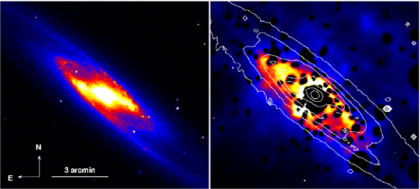
Figure 9: Comparison between the K-band (left, 2MASS, Jarrett et al., 2003) and X-ray (right) morphology. The white contours overplotted on the X-ray image represent the K-band brightness levels. Both images are on a linear colour scale, and on the same spatial scale as indicated in the K-band image.

In this section we investigate the possibility that the observed diffuse emission originates in fact not from a truly diffuse hot interstellar gas component, but from a large population of weak stellar-type X-ray sources that shows the same characteristics.

This effect was first discovered in the Milky Way’s ridge X-ray emission (e.g. Revnivtsev et al., 2006), where evidence was found that the bulk of the Galactic ridge X-ray emission is composed of weak X-ray sources, mostly cataclysmic variables and coronally active binary systems, with a luminosity of most of these sources of less than $10^{31}$ erg s^-1. Also in other galaxies, Revnivtsev et al. (2007) found that the apparently diffuse emission is consistent with the emission from an old stellar population like in the Milky Way.

Following the method by Revnivtsev et al. (2007), we used K-band observations, to infer the emissivity of the diffuse X-ray component per unit stellar mass. We derived the near-infrared luminosity and stellar mass of NGC 253, using the total K-band magnitude of 3.772 (Jarrett et al., 2003), the distance modulus of 27.06, corrected for interstellar extinction of 0.007 (Schlegel et al., 1998), and the colour-dependent K-band mass-to-light ratio from Bell & de Jong (2001), $\log(M_{*}/L_{\rm{K}})=-0.692+0.652\times(B-V)$, with $(B-V)=-0.16$ (Comerón et al., 2003). This yielded a total K-band luminosity $L_{\rm{K}}=1.6\times 10^{11}$ $L$_⊙ and a total stellar mass $M_{*}=2.6\times 10^{10}$ $M$_⊙. With a X-ray luminosity of NGC 253 of 2.0$\times 10^{39}$ erg s^-1 (0.5–10 keV), the emissivity of the diffuse X-ray component per unit stellar mass then resulted in

$$\frac{L_{0.5-10\,\,\mathrm{keV}}}{M_{*}}=7.6^{+0.9}_{-0.3}\,(\pm 2.3)\times 10^{28}\,\,\mathrm{erg}\,\,\mathrm{s}^{-1}\,\,M^{-1}_{\odot}.$$

The errors are statistical errors on the measured X-ray flux. Additionally, we assumed an uncertainty of $\sim$30% (given in parentheses), which might be associated with the $L_{\mathrm{K}}$ to $M_{*}$ conversion (Bell et al., 2003). The emissivity of NGC 253 should only be considered a lower limit. We cut out a quite large region in the centre of NGC 253 and corrected for this by filling the hole with the average flux of the disc. Therefore, the obtained X-ray luminosity as well as the emissivity are probably underestimated.

From the luminosity and other properties of the Galactic ridge X-ray emission (e.g. Revnivtsev et al., 2006) and from direct measurements of the luminosity function of sources in the solar neighbourhood (Sazonov et al., 2006), the combined 0.5–10 keV emissivity of cataclysmic variables and coronally active stars has been estimated as $L_{\mathrm{X}}/M_{*}\sim 1.2\pm 0.3\times 10^{28}\,\,\mathrm{erg}\,\,\mathrm{s}^{-1}\,\,M^{-1}_{\odot}$. The value derived for NGC 253 is larger than the value for the Milky Way, indicating the presence of a hot gaseous component.

An even stronger argument is the following: if the diffuse X-ray emission is produced by an old stellar population, then their morphologies should be similar. A comparison of the X-ray emission with the 2MASS K-band image (Jarrett et al., 2003) is shown in Fig. 9. We found that the X-ray morphology does not match the K-band morphology, therefore the diffuse emission is indeed not simply due to an old stellar population, but has to have a truly diffuse component.

4.3 Spectral fits and variations in the halo

As it was mentioned already in earlier publications, there is an ambiguity in the spectral fits between a pure multi-temperature thermal plasma model and a combination of thermal plasmas plus a power law component (e.g. Dahlem et al., 2000; Strickland et al., 2002). This ambiguity in the halo emission still exists with the XMM-Newton data. Fits to the halo spectra with a thermal plasma plus a power law model (see Table LABEL:tab:HaloFits) resulted in similar $\chi^{2}_{\nu}$, as for a multi-temperature thermal plasma model. A power law component from point sources could be excluded, since we were careful to remove any point source contribution. Another source for non-thermal emission could be synchrotron emission from cosmic ray electrons that are advected with the superwind or are accelerated locally in internal wind shocks. This is possibly what we observe in the spectrum of region 6 (and spectra containing region 6). This region lies along the northwestern outflow axis. Here the spectral fit improves significantly by adding a power law component to the two thermal plasmas. A comparison of the X-ray emission to the 330 MHz and 1.4 GHz radio emission (Carilli et al., 1992) showed that the radio emission is more extended, and does not show the horn structure that we see in X-rays. Because of this inequality, we prefer the multi-temperature thermal plasma over the single temperature model plus power law model for most of the X-ray halo emission at the moment.

The appearance of a “multi-temperature” halo is a natural consequence of the plasma driven out of collisional ionisation equilibrium (CIE) towards a non-equilibrium ionisation (NEI) state in a galactic outflow. It has to be borne in mind that the processes of ionisation, recombination and adiabatic cooling occur all on different time scales. Whereas the former two are controlled by microphysics the latter is due to the hydrodynamics of the flow. As has been described by e.g. Breitschwerdt & Schmutzler (1994) adiabatic cooling can become the shortest in an accelerating outflow, like the one occurring in a starburst driven wind, leading to delayed recombination of the plasma. This means essentially the presence of highly ionised species in a plasma flow with low kinetic electron temperature, similar to the ions in the solar wind. Releasing the energy stored in these highly ionised species results in diffuse soft X-ray emission and some spectral hardening. Observing this with the limited spectral resolution of Chandra or XMM-Newton CCDs, reveals a multi-temperature halo, although physically the plasma does by no means have “different temperatures”, but is characterised by a non-equilibrium distribution of ions, which by itself is the result of the thermodynamic path the system has taken and reflects directly the hydrodynamic flow characteristics. A currently ongoing analysis with non-equilibrium models (e.g. Breitschwerdt & Schmutzler, 1999) might also be able to explain the observations and is the subject of a forthcoming paper.

The northwestern halo shows significant hardness variations in HR1, as opposed to the findings by Strickland et al. (2002). We checked if this can be caused by a different energy band selection, but the result is independent whether we use the bands from Strickland et al. (2002) (0.3–0.6 keV and 0.6–1.0 keV) or our own. These hardness variations might also be a sign of NEI X-ray emission.

4.4 Temperatures, abundances and column densities

The X-ray emission from NGC 253 has been observed before with several other X-ray observatories. Especially the early observatories did not allow to separate the point sources from the diffuse emission since the point spread function was quite large. Hence, only a combined fit of the emission from the halo, the disc, and the nuclear region was possible. Temperatures of multi-temperature models ranged between 0.1 and 0.3 keV for the low, and between 0.6 and 0.7 keV for the high temperature component (Dahlem et al., 1998; Weaver et al., 2000; Dahlem et al., 2000). Reported abundances were mostly highly subsolar and therefore unphysical for a supposedly metal enriched starburst galaxy plasma.

Only the X-ray observatories like XMM-Newton, Chandra, and to some degree ROSAT allow us to separate the halo from the disc emission and to remove contribution by point sources via a spatial selection. From ROSAT data, Pietsch et al. (2000) inferred a foreground absorbed two-temperature thermal model with temperatures of 0.13 and 0.62 keV for the northwestern halo emission. No highly subsolar abundances were required. The disc emission could be explained by a 0.7 keV thermal plasma and an additional thermal plasma (kT=0.2 keV) in front of the disc coming from a coronal component.

The first XMM-Newton results by Pietsch et al. (2001) required a two-component model for the disc emission with temperatures of 0.13 and 0.4 keV plus residual harder emission, possibly from unresolved point sources. For the nuclear region three temperatures were needed (0.6, 0.9, and 6 keV). Both models used solar abundances. No analysis of the halo emission was presented in their paper.

The best spatial resolution is provided by the Chandra observatory. Results on the diffuse disc and halo emission were first published by Strickland et al. (2002). For the halo emission they needed a multi-temperature model (apec) with at least two temperatures of 0.24 and 0.71 keV (the latter with quite large errors) and with a foreground absorption of $5.3\times 10^{20}$ cm^-2. A power law ($\Gamma=3.3$) plus a thermal plasma (kT=0.24 keV) gave a similarly good fit. A combination of other thermal models (mekal) or non-equilibrium models (vnei) did not result in better fits. The diffuse emission from the disc was fitted with the same models, however, the temperatures were lower than in the halo, with 0.17 and 0.56 keV, respectively. The foreground absorption yields $4.7\times 10^{20}$ cm^-2. In all cases unphysically sub-solar abundances had to be assumed.

The temperature values for the halo emission, as found by our analysis, are lower than the ones from previous observations. Our soft component is about 0.10 keV, which is still compatible with the ROSAT results. However, the hard component is only $\sim$0.31 keV for the northwestern halo and $\sim$0.29 keV for the southeastern halo. A higher temperature was not necessary in any of our fits. A possible explanation could be the way the spectra were background subtracted. We used a sophisticated method (see App. B) that uses the local background at the border of the field of view, where no emission from NGC 253 is expected, while other authors used e.g. blank-sky observations (Strickland et al., 2002). Using a background from different times and different fields on the sky can lead to systematic effects in the background substraction. A background region with a higher contribution of the local bubble could, for example, lead to an over-correction, especially at very soft energies ($<$0.5 keV).

In the disc we found temperatures between 0.1 and 0.3 keV and between 0.3 and 0.9 keV, for the soft and the hard component, respectively. This is consistent with earlier results.

We also tried to constrain the metal abundances in our fits. However the errors on the obtained values are so large, that we are not able to give well constrained abundances (northwestern halo: $Z=0.3^{+4.7}_{-0.2}$ $Z$_⊙, southeastern halo: $Z=0.4^{+4.6}_{-0.3}$ $Z$_⊙, disc: $Z=1.0^{+0.9}_{-0.7}$ $Z$_⊙). Since we do not expect highly subsolar abundances in an environment which is enriched with metals from the starburst via the superwind and galactic fountains, we fixed the abundances in our analysis to solar. This is entirely consistent with the above values. A reason for the low abundances, found with different instruments, could be that due to a lower spatial resolution and or/and sensitivity more point sources contribute to the final spectrum, increasing the continuum flux. The ratio of line emission to continuum flux is therefore decreased, which mimics the spectral shape of a plasma with low metal abundances. A similar effect can be achieved when a NEI spectrum is fitted with CIE models. Also, a too simplistic model could be the reason, combining regions with different temperatures.

In the disc, two of the regions required an extra absorption component in the spectral model. The additional column densities range between 0.76$\times 10^{21}$ cm^-2 and 5.8$\times 10^{21}$ cm^-2. Direct radio measurements of the H I column density showed lower values than we derived from the X-ray data. An interpolation of the H I maps by Puche et al. (1991) and Koribalski et al. (1995) resulted in ($\sim$2.4 and 3.4)$\times 10^{21}$ cm^-2 for regions 9 and 16, respectively. However, the H I value for the region including the nucleus of NGC 253 (region 16) is affected by H I absorption, so the resulting column density can only be considered as a lower limit. Additional absorption is expected from molecular hydrogen. Mauersberger et al. (1995) derived the H₂ column density in the direction of the nucleus of NGC 253 to 3.7$\times 10^{23}$ cm^-2. Taking this value as an upper limit for the column density in the disc regions around the nucleus, the column densities derived from X-ray spectra are within the limits from radio observations.

4.5 X-ray versus UV morphology

Figure 10: Two-colour UV image of NGC 253 with NUV (175–280 nm) in yellow and FUV (135–175 nm) in blue. The intensity was rescaled to emphasise the faint, diffuse emission. Overplotted are the 0.2–0.5 keV X-ray contours.

Fig. 10 shows the X-ray contours from the energy band 0.2–0.5 keV overplotted on a two-colour UV image, taken with the GALEX observatory (Galaxy Evolution Explorer, a UV space telescope) on 2003 October 13. For the northwestern halo there is quite a good agreement between the FUV and X-ray emission regions. The FUV emission traces the western horn to a distance of $\sim$7.5 kpc above the disc, as well as the broad base emission in soft X-rays quite well. In the southeastern halo, again, the UV and the soft X-ray emission show the western horn structure, where the UV horn extends to about 7 kpc away from the disc. However, the FUV horn is slightly offset by $\sim$700 pc to the northeast with respect to the X-ray horn. Images obtained with the Optical Monitor onboard XMM-Newton are not sensitive enough to show the extraplanar UV emission.

Hoopes et al. (2005) proposed the following model for the origin of the UV emission: Since the UV luminosities are too high to to be produced by continuum and line emission from photoionised or shock-heated gas, the UV emission could be explained by dust in the outflow that scatters the stellar continuum from the starburst into our line of sight. They also found that the UV halo emission, as seen with GALEX, correlates with the H$\alpha$ emission, which could originate from gas that is photoionised by UV photons from the starburst. The UV and H$\alpha$ emission would originate in the same cold regions in the halo.

How does the warm gas that is responsible for the H$\alpha$ and UV emission get out into the halo? There are two possibilities: either it has already been there from the beginning in the form of a cold and maybe clumpy halo component, or it was transported by the superwind and galactic fountains from the disc out into the halo.

There are models, where it is possible to drag up clouds of cold gas into the halo (e.g. model 3 of Strickland et al., 2002). In a sheet surrounding these clouds, X-ray emission could be produced by shocks or in conductive or turbulent mixing interfaces on the cloud surface. This model would also account for the non-uniformity of the X-ray emission as seen in the XMM-Newton images (Fig. 1 and 3). However, the model cannot explain the displacement of the UV emission in the southeastern halo, since in the model the clouds are located within or at the inner border of the superwind.

Could the dust even survive this transport from the disc into the halo embedded in a hot plasma environment? Draine & Salpeter (1979) give the sputtering time for a spherical dust grain of radius $a$ embedded in a plasma of hydrogen with temperatures between $10^{6}$ and $10^{9}$ K and the density $n_{\mathrm{H}}$ as

$$t_{\mathrm{sput}}\sim 10^{6}\left(\frac{a}{\mu\mathrm{m}}\right)\left(\frac{n_{\mathrm{H}}}{\mathrm{cm}^{-3}}\right)^{-1}\,\mathrm{yr}.$$ (1)

For $n_{\mathrm{H}}$ between $2.5\times 10^{-2}$ cm^-3 in the outflow close to the centre (Bauer et al., 2007) and $3.2\times 10^{-3}$ cm^-3 out in the northwestern halo, and a grain size of $a$=0.1 $\mu$m, $t_{\mathrm{sput}}$ varies between 4.0 and 31 Myr. So to reach a height above the disc of 7.5 kpc in less than 31 Myr, an average velocity of at least 240 km/s is required. This is well compatible with measurements of outflow velocities in different wavelengths, that range from 260 km/s (Na D absorption, Heckman et al., 2000) to about 400–600 km/s (H$\alpha$, N II, S II, and O II emission, Ulrich, 1978; Demoulin & Burbidge, 1970). Therefore it is quite possible that the dust survives the transport from the disc out into the halo.

Another model to explain the UV and X-ray morphology (e.g. model 5 of Strickland et al., 2002) requires a thick disc component, through which the superwind emerges into the halo. On the contact surface between the hot superwind fluid and the cold thick disc material we get a heated layer through shocks and turbulent mixing where the X-rays are produced, surrounded on the outside by a colder layer where the UV emission originates. The thick disc component was originally created by lifting material up from the disc through the star formation activity (simulations by Rosen & Bregman, 1995). This model would easily explain the UV displacement from the X-rays, however we would only get a hollow cone with X-ray emission. The latter is not what we see in the XMM-Newton observations. Though a mix of both models would be able to explain the observed morphology.

For completeness, the three other models that Strickland et al. (2002) present are:

(i) Shocked clouds in the halo (model 2). In this model preexisting neutral clouds are overrun by the superwind, which can explain the often asymmetrical patchiness as a result of the spatial distribution of the clouds. However, no H I structures outside the disc have been found by Puche et al. (1991) and Koribalski et al. (1995).

(ii) Hot swept-up shell of halo gas (model 4). In this model a superbubble bounded by a shock expands into the low-density halo medium. The X-ray radiation originates from the shocked ambient gas following the morphology of the surface of the superbubble. Possible UV/H$\alpha$ emission could originate from dense cool disc gas entrained in the wind. Especially this last aspect is not supported by the observations.

(iii) Cooling radiation from the wind (model 1). As presented by Strickland et al. (2002) this model cannot explain the UV or H$\alpha$ emission, and also does not explain the horn shaped morphology of both the X-ray and UV emission.

The magnetohydrodynamics ISM simulations of de Avillez & Breitschwerdt (2005) also shows a clumpy halo structure, characterised by turbulent mixing layers, which could explain the UV and X-ray filamentary structure. In some regions, the magnetic field forms loops surrounded by shells which may exhibit enhanced UV emission.

5 Summary

We have characterised the diffuse emission in NGC 253. The disc extends 13.6 kpc along the major axis and shows emission between 0.2 and 10 keV. The spectrum could be modelled with two thermal plasmas ($T_{\mathrm{cold}}=0.1-0.3$ keV and $T_{\mathrm{hot}}=0.3-0.9$ keV) with solar abundances plus a power law component and galactic foreground absorption. The power law component may indicate an unresolved contribution from X-ray binaries in the disc. The total luminosity of the diffuse emission in the disc is 2.4$\times 10^{39}$ erg s^-1 (0.2-10.0 keV). We found clear evidence for hot plasma in the disc. The diffuse emission does not originate completely from an old stellar population.

The halo resembles a horn structure which reaches out to a projected height of $\sim$9 kpc perpendicular to the disc. The halo emission on smaller scales seems not to be uniformly distributed, but shows a filamentary structure. The southeastern halo is softer than the northwestern halo. To model the spectra in the halo we needed two thermal plasmas ($T_{\mathrm{cold}}\sim 0.1$ keV and $T_{\mathrm{hot}}\sim 0.3$ keV) with solar abundances plus galactic foreground absorption, which is an indication for the non-equilibrium ionisation state of the halo plasma. The total luminosity of the diffuse emission is 8.4$\times 10^{38}$ erg s^-1 and 2.3$\times 10^{38}$ erg s^-1 (0.2-1.5 keV) in the northwestern and southeastern halo, respectively. Densities computed to $3.2\,\eta^{-0.5}\times 10^{-3}$ cm^-3 and $4.7\,\eta^{-0.5}\times 10^{-3}$ cm^-3, with the volume filling factor $\eta$. With solar abundances this implies total masses of $3.3\,\eta^{-0.5}\times 10^{7}$ M_☉ and $1.8\,\eta^{-0.5}\times 10^{7}$ M_☉ for the northwestern and southeastern halo, respectively.

A comparison between X-ray and UV emission showed that both originate from the same regions. The UV emission is more extended in the southeastern halo, where it seems to form a shell around the X-ray emission.

Appendix A EPIC pn images

We developed an algorithm to create vignetting corrected and adaptively smoothed EPIC pn images. This procedure is based on the observation itself. Specifically, closed filter observations were not used in addition. In the following we will describe the algorithm step-by-step.

The basis for this procedure is a cleaned event file and an out-of-time event file. This cleaning included screening for high background and also removing bad pixels and bad columns. If we want to use more than one observation, all steps have to be performed for all observations separately, before the products are merged.

We will here concentrate on the creation of three images, which can be combined to a RGB colour image at the end of the procedure. In the following all steps are to be done for all three energy bands, unless stated otherwise.

For the desired energy band, we extracted an image from the event file. This image was then corrected for out-of-time events, via subtraction of an image that was extracted from the out-of-time event file and rescaled with the out-of-time event fraction. Next, we corrected for the detector background (electronic noise, high energy particles) by subtracting the detector background surface brightness from the image. This value was determined from the corners of the detector which are outside of the field of view of the telescope. We here assumed that the detector background is uniform across the whole detector (for energies above $\sim$7.2 keV this is no longer a good approximation, see Freyberg et al. 2004).

We created vignetting corrected exposure maps and masks using the SAS-tasks eexpmap and emask, respectively, which will be used to account for differences in the exposure times in the images, and to mask the images to regions with an acceptable minimum exposure time. Before we could smooth the image adaptively, we had to create a template with smoothing kernels. This template guarantees that images in different energy bands are smoothed with the same kernel size. Therefore we added up the images in the different energy bands. With the task asmooth, we created the template using the merged image, the merged mask, and an exposure map.

Now we have all the necessary products to smooth the single images. We smoothed the images in the different energy bands with the smoothing template, the vignetting corrected exposure map, and with the corresponding mask. This step included the vignetting correction via the exposure map, and a masking of the image to a region with an acceptable minimum exposure time.

In a final step we used ds9 to create the RGB colour image. The resulting images of NGC 253 and a combined RGB colour image of the lowest three energy bands is shown in Fig. 1 and 3.

Appendix B Background spectra

$$\begin{split}B(E)&=\underbrace{S^{\mathrm{OOT}}_{\mathrm{obs}}(E)\times f}_{\mathrm{Out-of-Time\,\,\,events}}+\underbrace{S_{\mathrm{det}}(E)\frac{R_{\mathrm{obs}}}{R_{\mathrm{det}}}\frac{t_{\mathrm{obs}}}{t_{\mathrm{det}}}}_{\mathrm{detector\,\,\,background}}-\underbrace{S^{\mathrm{OOT}}_{\mathrm{det}}(E)\frac{R_{\mathrm{obs}}}{R_{\mathrm{det}}}\frac{t_{\mathrm{obs}}}{t_{\mathrm{det}}}\times f}_{\mathrm{detector\,\,Out-of-Time\,\,events}}+\\ &+\underbrace{\frac{V(E,\theta_{S})}{V(E,\theta_{B})}\frac{A_{S}}{A_{B}}\times\left(B_{\mathrm{obs}}(E)-\underbrace{B^{\mathrm{OOT}}_{\mathrm{obs}}(E)\times f}_{\mathrm{Out-of-Time\,\,\,events}}-\underbrace{B_{\mathrm{det}}(E)\frac{R_{\mathrm{obs}}}{R_{\mathrm{det}}}\frac{t_{\mathrm{obs}}}{t_{\mathrm{det}}}}_{\mathrm{detector\,\,\,background}}+\underbrace{B^{\mathrm{OOT}}_{\mathrm{det}}(E)\frac{R_{\mathrm{obs}}}{R_{\mathrm{det}}}\frac{t_{\mathrm{obs}}}{t_{\mathrm{det}}}\times f}_{\mathrm{detector\,\,Out-of-time\,\,events}}\right)}_{\mathrm{sky\,\,background}}\\ \end{split}$$ (2)

The conventional way to create a background spectrum is to select a region from the same observation where there is no emission from the source. Additionally, the region should be close to the source. This way, the spectral background should have the same characteristics as the background at the source region. In NGC 253, a region which suffices the first criterion can be found at the border of the field of view in the southwestern part of the detector. The second criterion, however, is not satisfied. The background region may show a different detector background, and additionally the vignetting is different.

Table 6: Rejected CCD rows due to MIPs per time unit in the used observations.

Obs ID	Filter	rejected line counter value
0122320707	Closed	181.7
0125960101	Medium	190.2
0152020101	Thin	141.4
0160362801	Closed	120.4

Since we were interested in determining the characteristics of emission with low surface brightness, that extends over a large region, where the background is (probably) the dominant component, we needed a very accurate estimate of the background. Given the very soft nature of the emission, we cannot use blank sky observations that were taken in regions of the sky where the foreground $N_{\rm H}$ is different (not to mention other uncertainties due to different detector settings, particle radiation levels, etc.). Here we describe a method to use a local estimate of the sky background that takes properly into account vignetting and detector background issues.

To remove the detector background, we used archival observations which were taken in the same mode as the NGC 253 observations, but where the filter wheel was closed. To avoid effects due to changes in the detector settings, or changes of the detector performance due to other reasons, we chose the closed observations to be as close as possible in time to the NGC 253 observations. The closed observations we used for observation 1 and 4 are: revolution 59, obs. id. 0122320701, exposure S003 (50.5 ks) and revolution 732, obs. id. 0160362801, exposure S005 (38.6 ks), respectively. To ensure, that there are as little as possible differences between the source observation and the closed observation, we removed bad columns and bad pixels both in the NGC 253 and closed observation. Additionally, the closed observations may have been taken when the spacecraft was exposed to a different particle radiation level than the one present during observations 1 or 4. The XMM-Newton house keeping file contains information on how many CCD rows per time unit were rejected due to a possible minimum ionising particle (MIP) event, which is a direct estimator of the average radiation level. We used these values (see Table 6), to rescale the count rate of the closed observations.

We used Out-of-Time spectra from the source and background region to correct for contribution from Out-of-Time events. When one subtracts a closed observation spectrum from a Out-of-Time corrected spectrum, one actually removes the Out-of-Time spectrum of the detector background twice. This is corrected in our method by adding again the Out-of-Time spectra of the detector background.

We corrected the background region spectrum for Out-of-Time events and the detector background and applied the vignetting correction in each energy bin as a function of off-axis angle of the source and background spectrum. This gave us the sky background spectrum.

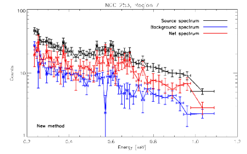
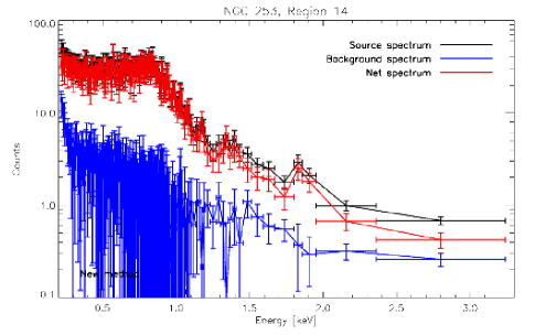
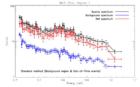
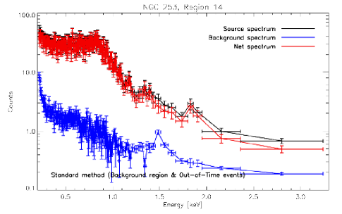
Figure 11: Comparison between the background substraction on two examples. (left): the spectrum of region 7, (right): the spectrum of region 14. The top panel shows the new method, as described in this paper, the bottom panel shows the conventional method, where the raw background spectrum is used, and a correction for Out-of-Time events has been applied. We only show the spectra of observation 4 here, since these have the better statistics.

In all of the above steps, different exposure times and areas in the extraction regions have been accounted for. Since some of the components in the final background spectrum do have low number statistics, we used the conservative approximation to Poissonian errors $\sigma_{N}\approx 1+\sqrt{0.75+N}$ (Gehrels 1986). To avoid unjustified large errors, we roughly binned the spectrum before calculating errors. This binning to a significance of $>3\,\sigma$ in each bin is performed on the conventionally background subtracted source spectrum (no vignetting correction and no closed observations) and guarantees that the final background subtracted spectrum then has a significance in each bin of a least 3 $\sigma$. The errors were propagated properly and were included in the file with the final background spectrum. This spectrum can be used with XSPEC as a background spectrum.

The whole method can be summarised by Eq. 2 with the following symbols:

• $B(E)$ is the counts at energy $E$ in the background spectrum

• $B_{\mathrm{obs}}(E)$ is the counts in the NGC 253 observation

• $S_{\mathrm{det}}(E)$ is the counts from the detector background spectrum in the source region

• $B_{\mathrm{obs}}(E)$ is the counts in the detector background spectrum in the background region

• $S^{\mathrm{OOT}}_{\mathrm{obs}}(E)$ are the counts in the Out-of-Time spectra in the source region

• $B^{\mathrm{OOT}}_{\mathrm{obs}}(E)$ are the counts in the Out-of-Time spectra in the background region

• $t_{\mathrm{obs}}$ is the exposure time in the NGC 253 observation

• $t_{\mathrm{det}}$ is the exposure time in the closed observation

• $R_{\mathrm{obs}}$ is the rejected line counter values (see Table 6) in the NGC 253 observation

• $R_{\mathrm{det}}$ is the rejected line counter values (see Table 6) in the closed observation

• $A_{S}$ is the area in the source region

• $A_{B}$ is the area in the background region

• $V(E,\theta_{S})$ is the vignetting value in the source region, depending on the offset angle $\theta$ and the energy $E$

• $V(E,\theta_{B})$ is the vignetting value in the background region, depending on the offset angle $\theta$ and the energy $E$

• $f$ is the fraction of Out-of-Time events in the corresponding mode of the observation

A comparison between this new method and the conventional method, that does not use the vignetting correction nor the closed observations, is shown in Fig. 11 for two example spectra, both in observations 1 and 4. The single background components in the source and background region in observation 4 are shown in Fig. 12. All figures show counts integrated over the extraction region. The counts in the background region were rescaled to the source region area to be able to compare them to the source spectrum. Also, the counts in the closed observation were rescaled to the exposure time and radiation level in the source observation.

The differences between the new and the conventional method in terms of the resulting best fits are the following: In the majority of the tested cases, an additional power law component with $\Gamma\sim 0$ is required for the fit in the spectrum, obtained with the conventional method. The temperatures are consistent between both methods, but the resulting flux levels in the conventional method are higher. Differences in total flux values range between 2% and 22%. The effect between the two methods is highest in regions with low surface brightness. Here the background dominates and a correct treatment is crucial. As an example, the difference in flux in region 7 (low surface brightness) is 15% and 22%, for observations 1 and 4, respectively. Whereas in region 14 (high surface brightness), the differences are 2% and 3%.

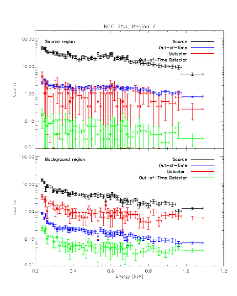
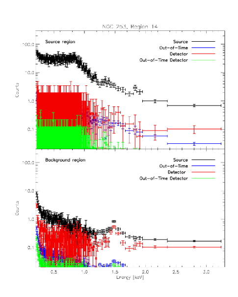
Figure 12: The single components that are part of the total background spectrum compared to the source spectrum. (left): Region 7, (right): Region 14, (top): components from the source region, (bottom): components from the background region. The single components were corrected for areas, exposure time, and radiation level, with respect to the source spectrum in the source region, but no vignetting correction was applied yet.