Abstract

An inclusion of temperature and chemical potential dependent surface tension into the gas of quark-gluon bags model resolves a long standing problem of a unified description of the first and second order phase transition with the cross-over. The suggested model has an exact analytical solution and allows one to rigorously study the vicinity of the critical endpoint of the deconfinement phase transition. It is found that at the curve of a zero surface tension coefficient there must exist the surface induced phase tranition of the 2^nd or higher order. The present model predicts that the critical endpoint (CEP) of quantum chromodynamics is the tricritical endpoint.

1 Introduction

The role of surface tension for the quark gluon plasma (QGP) was discussed long ago [1, 2], however, up to now the situation is somewhat unclear [3, 4]. In nuclear and cluster physics the importance of the surface tension for the properties of CEP is known from a number of exactly solvable cluster models with the 1^st order phase transition (PT) which describe the critical point properties very well. These models are built on the assumptions that the difference of the bulk part (or the volume dependent part) of free energy of two phases disappears at phase equilibrium and that, in addition, the difference of the surface part (or the surface tension) of free energy vanishes at the critical point. The most famous of them is the Fisher droplet model (FDM) [6, 7] which has been successfully used to analyze the condensation of a gaseous phase (droplets of all sizes) into a liquid.

Another such a model is a simplified version of the statistical multifragmentation model (SMM) [8] which was solved analytically both for infinite [9, 10] and for finite [11, 12] volumes of the system. The analysis of critical indices of the SMM [10] shows that the value of Fisher exponent $\tau_{SMM}=1.825\pm 0.025$ of this model is consistent with ISiS Collaboration data [13] and EOS Collaboration data [14]. Such an experimentally obtained range of the $\tau$ index is of a principal importance because it gives a very strong evidence that the SMM, and, thus, the nuclear matter, has a tricritical endpoint rather than a critical endpoint [9, 10].

This success of the SMM initiated the studies of the surface partitions of large clusters within the Hills and Dales Model [15, 16] and led to a discovery of the origin of the temperature independent surface entropy similar to the FDM. As a consequence, the surface tension coefficient of large clusters consisting of the discrete constituents should linearly depend on the temperature of the system [15] and must vanish at the critical endpoint. However, the present formulation of the Hills and Dales Model [15, 16], which successfully estimates the upper and lower bounds of the surface deformations of the discrete physical clusters, does not look suitable for quark-gluon bags. Therefore, in this work I insert the surface tension into the gas of bags model (GBM) [17], assume a certain dependence of the surface tension coefficient on temperature and baryonic chemical potential. Then I analyze the quark gluon bags with surface tension (QGBST) model and concentrate on the impact of surface tension on the properties of the deconfinement phase diagram and the QCD critical endpoint.

Here I show that at low values of the baryonic chemical potential the 1^st order deconfinement PT degenerates into a cross-over, if the surface tension coefficient becomes negative for lower values of temperature than the transition temperature. Also I prove the existence of an additional PT of the 2^nd or higher order along the curve where the surface tension coefficient vanishes. Thus, I am arguing that the QGBST model predicts the existence of the tricritical rather than critical endpoint.

2 The Role of Surface Tension at Zero Baryonic Densities

The isobaric partition of the QGBST model obtained from the grand canonical one $Z(V,T)$ is as follows

$$\hat{Z}(s,T)\equiv\int\limits_{0}^{\infty}dV\exp(-sV)~{}Z(V,T)=\frac{1}{[s-F(s,T)]}\,.$$ (1)

Here the function $F(s,T)$ consists of two parts, the discrete mass-volume spectrum $F_{H}(s,T)$, and the continuous part of the spectrum $F_{Q}(s,T)$

$$F(s,T) \equiv\sum_{j=1}^{n}~{}\phi(T,m_{j})e^{-v_{j}s}+~{}u(T)~{}\int\limits_{V_{0}}^{\infty}dv~{}\frac{\exp\left[\left(s_{Q}(T)-s\right)v-\sigma(T)\,v^{\kappa}\right]}{v^{\tau}}~{},$$ (2)

where the function $\phi(T,m_{k})\equiv\frac{g_{k}}{2\pi^{2}}\int\limits_{0}^{\infty}p^{2}dp~{}e^{\textstyle-\frac{(p^{2}~{}+~{}m_{k}^{2})^{1/2}}{T}}=g_{k}\frac{m_{k}^{2}T}{2\pi^{2}}~{}{K}_{2}\left(\frac{m_{k}}{T}\right)$ is the particle density of bags of mass $m_{k}$ and eigen volume $v_{k}$ and degeneracy $g_{k}$.

At the moment the particular choice of function $F_{Q}(s,T)$ in (2) is not important. The key point of my treatment is that it should have the form of Eq. (2) which has a singularity at $s=s_{Q}^{*}$ because for $s<s_{Q}$ the integral over the bag volume $v$ diverges at its upper limit. As will be shown below the isobaric partition (1) has two kind of singularities: the simple pole $s=s_{H}^{*}$ and the essential singularity $s=s_{Q}$ The rightmost singularity defines the phase in which matter exists, whereas a PT occurs when two singularities coincide [17, 9, 3]. All singularities are defined by the equation

$$s^{*}~{} = ~{}{F(s^{*},T)}\,.$$ (3)

The $v$-linear term in the exponential of the continuous spectrum (2) is nothing else, but a difference of the bulk free energy of a bag of volume $v$, i.e. $-Tsv$, which is under external pressure $Ts$, and the bulk free energy of the same bag filled with QGP, i.e. $-Ts_{Q}v$. The term $-Tsv$ appears due to the hard core repulsion [3], whereas the QGP pressure, $Ts_{Q}$, appears in (2) as a generalization of the Hagedorn mass spectrum [18]. At phase equilibrium this difference of the bulk free energies vanishes and the properties of phase equilibrium are defined by the surface free energy.

Note that the usage of the grand canonical description for the exponential mass or volume spectrum of Hagedorn type was strongly criticized recently [4, 5, 19, 20, 21] because of the thermostatic properties of this spectrum. However, the hard core repulsion compensates the growing part of the mass-volume spectrum and, hence, the criticism of Refs. [4, 5, 19, 20, 21] is irrelevant to the present model.

The new element in (2) is the presence of surface free energy $\sigma_{0}v^{\kappa}$ (${\kappa}<1$) of the bag. The power $\kappa<1$ which describes the bag’s effective surface is a constant which, in principle, can differ from the typical FDM and SMM value $\frac{2}{3}$, if the highly non-sperical bags are possible [3, 7, 15, 16]. The ratio of the temperature dependent surface tension coefficient to $T$ (the reduced surface tension coefficient hereafter) which has the form $\sigma(T)=\frac{\sigma_{o}}{T}\cdot\left[\frac{T_{cep}-T}{T_{cep}}\right]^{2k+1}$ ($k=0,1,2,...$). Here $\sigma_{o}>0$ can be a smooth function of the temperature, but for simplicity I fix it to be a constant.

In choosing such a simple surface energy parameterization I follow the original Fisher idea [6] which allows one to account for the surface energy by considering some mean bag of volume $v$ and surface $v^{\kappa}$. The consideration of the general mass-volume-surface bag spectrum is reserved for the future investigation. In contrast to the FDM and SMM, the power $\kappa<1$ which describes the bag’s effective surface is a constant which, as mentioned above, can differ from the typical FDM and SMM value $\frac{2}{3}$. This is so because near the deconfinement PT region the QGP has low density and, hence, like in the low density nuclear matter [22], the non-sperical bags (spaghetti-like or lasagna-like [22]) can be favorable (see a [3] and references therein). A similar idea of “polymerization” of gluonic quasiparticles was introduced recently [23].

The second essential difference with the FDM and SMM surface tension parameterizations is that the vanishing of $\sigma(T)$ above the CEP temperature is not required. As will be shown later, this is the most important assumption which, in contrast to the GBM, allows one to naturally describe the cross-over from hadron gas to QGP. Note that negative value of the reduced surface tension coefficient $\sigma(T)$ above the CEP does not mean anything wrong. As discussed above, the surface tension coefficient consists of energy and entropy parts which have opposite signs [6, 15, 16]. Therefore, $\sigma(T)<0$ does not mean that the surface energy changes the sign, but it rather means that the surface entropy, i.e. the logarithm of the degeneracy of bags of a fixed volume, simply exceeds their surface energy. In other words, the number of non-spherical bags of a fixed volume becomes so large that the Boltzmann exponent, which accounts for the energy ”costs” of these bags, cannot suppress them anymore.

Finally, the third essential difference with the FDM and SMM is that it is assumed that the surface tension in the QGBST model vanishes at some line in $\mu_{B}-T$ plane, i.e. $T_{cep}=T_{cep}(\mu_{B})$. However, in the subsequent sections I will consider $T_{cep}=Const$ for simplicity, and in Sect. 4 I will discuss the necessary modifications of the model with $T_{cep}=T_{cep}(\mu_{B})$.

In principle, besides the bulk and surface parts of free energy, the continuous volume spectrum $F_{Q}(s,T)$ could include the curvature part as well, which may be important for small hadronic bubbles [24, 25, 26] or for cosmological PT [27]. It is necessary to stress, however, that the critical properties of the present model are defined by the infinite bag, therefore the inclusion into the function $F_{Q}(s,T)$ of a curvature term of bag’s free energy of any sign could affect the thermodynamic quantities of this model at $s=s_{Q}(T)$ and $\sigma(T)=0$, which is possible at (tri)critical endpoint only (see below). If, the curvature term was really important for the cluster models like the present one, then it should have been seen also at (tri)critical points of the FDM, SMM and many systems described by the FDM, but this is not the case [7, 28]. Indeed, recently the Complement method [28] was applied to the analysis of the largest, but still mesoscopic drop of a radius $R_{dr}$ representing the liquid in equilibrium with its vapor. The method allows one to find out the concentrations of the vapor clusters in finite system in a whole range of temperatures and determine the free energy difference of two phases with high precision. The latter enables us not only to extract the critical temperature, surface tension coefficient and even the value of Fisher index $\tau$ of the infinite system, but also such a delicate effects as the Gibbs-Thomson correction [29] to the free energy of a liquid drop. Note that the Gibbs-Thomson correction behaves as $R_{dr}^{-1}$, but the Complement method [28] allows one to find it, whereas the curvature part of free energy, which is proportional to $R_{dr}$, is not seen both for a drop and for smaller clusters. Such a result is directly related to the QGP bags because QCD is expected to be in the same universality class [30, 31] as the 3-dimensional Ising model whose clusters were analyzed in [28]. Therefore, admitting that for finite QGP bags the curvature effects may be essential, I leave them out because the critical behavior of the present model is defined by the properties of the infinite bag. On the other hand, similarly to the FDM, SMM and FDM-like systems discussed in Ref. [7], I assume that the curvature part of free energy of the infinite QGP bag is not important and leave for the future analysis the question why this is so.

According to the general theorem [17] the analysis of PT existence of the GCP is now reduced to the analysis of the rightmost singularity of the isobaric partition (1). Depending on the sign of the reduced surface tension coefficient, there are three possibilities.

(I) The first possibility corresponds to $\sigma(T)>0$. Its treatment is very similar to the GBM parameterization of continuous spectrum with $\tau>2$ [17]. In this case at low temperatures the QGP pressure $Ts_{Q}(T)$ is negative and, therefore, the rightmost singularity is a simple pole of the isobaric partition $s^{*}=s_{H}(T)=F(s_{H}(T),T)>s_{Q}(T)$, which is mainly defined by a discrete part of the volume spectrum $F_{H}(s,T)$. The last inequality provides the convergence of the volume integral in (2) (see Fig. 1). On the other hand at very high $T$ the QGP pressure dominates and, hence, the rightmost singularity is the essential singularity of the isobaric partition $s^{*}=s_{Q}(T)$. The phase transition occurs, when the singularities coincide:

$$s_{H}(T_{c})\equiv\frac{p_{H}(T_{c})}{T_{c}}=s_{Q}(T_{c})\equiv\frac{p_{Q}(T_{c})}{T_{c}}\,,$$ (4)

which is nothing else, but the Gibbs criterion. The graphical solution of Eq. (3) for all these possibilities is shown in Fig. 1. Like in the GBM [17], the necessary condition for the PT existence is the finiteness of $F_{Q}(s_{Q}(T),T)$ at $s=s_{Q}(T)$. It can be shown that the sufficient conditions are the following inequalities: $F_{Q}(s_{Q}(T),T)>s_{Q}(T)$ for low temperatures and $F(s_{Q}(T),T)<s_{Q}(T)$ for $T\rightarrow\infty$. These conditions provide that at low $T$ the rightmost singularity of the isobaric partition is a simple pole, whereas for hight $T$ the essential singularity $s_{Q}(T)$ becomes its rightmost one (see Fig. 1 and a detailed analysis of the case $\mu_{B}\neq 0$).

         

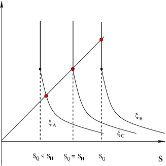
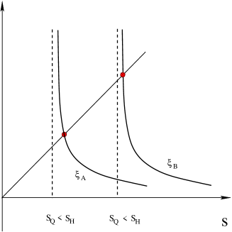
Figure 1: Left panel. Graphical solution of Eq. (3) which corresponds to a PT. The solution of Eq. (3) is shown by a filled hexagon. The function $F(s,\xi)$ is shown by a solid curve for a few values of the parameter $\xi$. The function $F(s,\xi)$ diverges for $s<s_{Q}(\xi)$ (shown by dashed lines), but is finite at $s=s_{Q}(\xi)$ (shown by black circle). At low values of the parameter $\xi=\xi_{A}$, which can be either $T$ or $\mu_{B}$, the simple pole $s_{H}$ is the rightmost singularity and it corresponds to hadronic phase. For $\xi=\xi_{B}\gg\xi_{A}$ the rightmost singularity is an essential singularity $s=s_{Q}(\xi_{B})$, which describes QGP. At intermediate value $\xi=\xi_{C}$ both singularities coincide $s_{H}(\xi_{C})=s_{Q}(\xi_{C})$ and this condition is a Gibbs criterion.
Right panel. Graphical solution of Eq. (3) which corresponds to a cross-over. The notations are the same as in the left panel. Now the function $F(s,\xi)$ diverges at $s=s_{Q}(\xi)$ (shown by dashed lines). In this case the simple pole $s_{H}$ is the rightmost singularity for any value of $\xi$.

The PT order can be found from the $T$-derivatives of $s_{H}(T)$. Thus, differentiating (3) one finds

$$s_{H}^{\prime}~{}=~{}\frac{G~{}+~{}u\,{\cal K}_{\tau-1}(\Delta,-\sigma)\cdot s_{Q}^{\prime}}{1~{}+~{}u\,{\cal K}_{\tau-1}(\Delta,-\sigma)}\,,$$ (5)

where the functions $G$ and ${\cal K}_{\tau-a}(\Delta,-\sigma)$ are defined as ($\Delta\equiv s_{H}-s_{Q}$)

$$G\equiv F_{H}^{\prime}+\frac{u^{\prime}}{u}F_{Q}+{\textstyle\frac{(T_{cep}-2kT)\sigma(T)}{(T_{cep}-T)\,T}}\,u\,{\cal K}_{\tau-\kappa}(\Delta,-\sigma)\,,$$ (6)

$${\cal K}_{\tau-a}(\Delta,-\sigma)\equiv\int\limits_{V_{o}}^{\infty}dv~{}\frac{\exp\left[-\Delta v-\sigma(T)v^{\kappa}\right]}{v^{\tau-a}}\,.$$ (7)

Now it is easy to see that the transition is of the 1^st order, i.e. $s_{Q}^{\prime}(T_{c})>s_{H}^{\prime}(T_{c})$, provided $\sigma(T)>0$ for any $\tau$. The 2^nd or higher order phase transition takes place provided $s_{Q}^{\prime}(T_{c})=s_{H}^{\prime}(T_{c})$ at $T=T_{c}$. The latter condition is satisfied when ${\cal K}_{\tau-1}$ diverges to infinity at $T\rightarrow(T_{c}-0)$, i.e. for $T$ approaching $T_{c}$ from below. Like for the GBM choice (2), such a situation can exist for $\sigma(T_{c})=0$ and $\frac{3}{2}<\tau\leq 2$. Studying the higher $T$-derivatives of $s_{H}(T)$ at $T_{c}$, one can show that for $\sigma(T)\equiv 0$ and for $(n+1)/n\leq\tau<n/(n-1)$ ($n=3,4,5,...$) there is a $n^{th}$ order phase transition

$$s_{H}(T_{c})=s_{Q}(T_{c}),~{}s_{H}^{\prime}(T_{c})=s_{Q}^{\prime}(T_{c}),~{}...~{}s_{H}^{(n-1)}(T_{c})=s_{Q}^{(n-1)}(T_{c}),~{}s_{H}^{(n)}(T_{c})\neq s_{Q}^{(n)}(T_{c}),$$ (8)

with $s_{H}^{(n)}(T_{c})=\infty$ for $(n+1)/n<\tau<n/(n-1)$ and with a finite value of $s_{H}^{(n)}(T_{c})$ for $\tau=(n+1)/n$.

(II) The second possibility, $\sigma(T)\equiv 0$, described in the preceding paragraph, does not give anything new compared to the GBM [17]. If the PT exists, then the graphical picture of singularities is basically similar to Fig. 1. The only difference is that, depending on the PT order, the derivatives of $F(s,T)$ function with respect to $s$ should diverge at $s=s_{Q}(T_{c})$.

(III) A principally new possibility exists for $T>T_{cep}$, where $\sigma(T)<0$. In this case there exists a cross-over, if for $T\leq T_{cep}$ the rightmost singularity is $s_{H}(T)$, which corresponds to the leftmost curve in the left panel of Fig. 1. Under the latter, its existence can be shown as follows. Let us solve the equation for singularities (3) graphically (see the right panel of Fig. 1). For $\sigma(T)<0$ the function $F_{Q}(s,T)$ diverges at $s=s_{Q}(T)$. On the other hand, the partial derivatives $\frac{\partial F_{H}(s,T)}{\partial s}<0$ and $\frac{\partial F_{Q}(s,T)}{\partial s}<0$ are always negative. Therefore, the function $F(s,T)\equiv F_{H}(s,T)+F_{Q}(s,T)$ is a monotonically decreasing function of $s$, which vanishes at $s\rightarrow\infty$. Since the left hand side of Eq. (3) is a monotonically increasing function of $s$, then there can exist a single intersection $s^{*}$ of $s$ and $F(s,T)$ functions. Moreover, for finite $s_{Q}(T)$ values this intersection can occur on the right hand side of the point $s=s_{Q}(T)$, i.e. $s^{*}>s_{Q}(T)$ (see the right panel of Fig. 1). Thus, in this case the essential singularity $s=s_{Q}(T)$ can become the rightmost one for infinite temperature only. In other words, the pressure of the pure QGP can be reached at infinite $T$, whereas for finite $T$ the hadronic mass spectrum gives a non-zero contribution into all thermodynamic functions. Note that such a behavior is typical for the lattice QCD data at zero baryonic chemical potential [32].

In terms of the present model it is clear that a cross-over existence means a fast transition of energy or entropy density in a narrow $T$ region from a dominance of the discrete mass-volume spectrum of light hadrons to a dominance of the continuous spectrum of heavy QGP bags. This is exactly the case for $\sigma(T)<0$ because in the right vicinity of the point $s=s_{Q}(T)$ the function $F(s,T)$ decreases very fast and then it gradually decreases as function of $s$-variable. Since, $F_{Q}(s,T)$ changes fast from $F(s,T)\sim F_{Q}(s,T)\sim s_{Q}(T)$ to $F(s,T)\sim F_{H}(s,T)\sim s_{H}(T)$, their $s$-derivatives should change fast as well. Now, recalling that the change from $F(s,T)\sim F_{Q}(s,T)$ behavior to $F(s,T)\sim F_{H}(s,T)$ in $s$-variable corresponds to the cooling of the system (see the right panel of Fig. 1), I conclude that that there exists a narrow region of temperatures, where the $T$ derivative of system pressure, i.e. the entropy density, drops down from $\frac{\partial p}{\partial T}\sim s_{Q}(T)+T\frac{ds_{Q}(T)}{dT}$ to $\frac{\partial p}{\partial T}\sim s_{H}(T)+T\frac{ds_{H}(T)}{dT}$ very fast compared to other regions of $T$, if system cools. If, however, in the vicinity of $T=T_{cep}-0$ the rightmost singularity is $s_{Q}(T)$, then for $T>T_{cep}$ the situation is different and the cross-over does not exist. A detailed analysis of this situation is given in Sect. 4.

Note also that all these nice properties would vanish, if the reduced surface tension coefficient is zero or positive above $T_{cep}$. This is one of the crucial points of the present model which puts forward certain doubts about the vanishing of the reduced surface tension coefficient in the FDM and SMM. These doubts are also supported by the first principle results obtained by the Hills and Dales Model [15, 16], because the surface entropy simply counts the degeneracy of a cluster of a fixed volume and it does not physically affect the surface energy of this cluster.

3 Generalization to Non-Zero Baryonic Densities

The possibilities (I)-(III) discussed in the preceding section remain unchanged for non-zero baryonic numbers. The latter should be included into consideration to make our model more realistic. To keep the presentation simple, I do not consider strangeness. The inclusion of the baryonic charge of the quark-gluon bags does not change the two types of singularities of the isobaric partition (1) and the corresponding equation for them (3), but it leads to the following modifications of the $F_{H}$ and $F_{Q}$ functions:

$$F_{H} (s,T,\mu_{B})=\sum_{j=1}^{n}g_{j}e^{\frac{b_{j}\mu_{B}}{T}-v_{j}s}\phi(T,m_{j})\,,$$ (9)

$$F_{Q} (s,T,\mu_{B})={\textstyle u(T,{\mu_{B}})}\int\limits_{V_{0}}^{\infty}dv~{}\frac{\exp\left[\left(s_{Q}(T,\mu_{B})-s\right)v-\sigma(T)v^{\kappa}\right]}{v^{\tau}}\,.$$ (10)

Here the baryonic chemical potential is denoted as $\mu_{B}$, the baryonic charge of the $j$-th hadron in the discrete part of the spectrum is $b_{j}$. The continuous part of the spectrum, $F_{Q}$ can be obtained from some spectrum $\rho(m,v,b)$ in the spirit of Ref. [33], but this is not the aim of the present work.

The QGP pressure $p_{Q}=Ts_{Q}(T,\mu_{B})$ can be also chosen in several ways. Here I use the bag model pressure

$$p_{Q}=\frac{\pi^{2}}{90}T^{4}\left[\frac{95}{2}+\frac{10}{\pi^{2}}\left(\frac{\mu_{B}}{T}\right)^{2}+\frac{5}{9\pi^{4}}\left(\frac{\mu_{B}}{T}\right)^{4}\right]-B\,,$$ (11)

but the more complicated model pressures, even with the PT of other kind like the transition between the color superconducting QGP and the usual QGP, can be, in principle, used.

It can be shown [3] that the sufficient conditions for a PT existence are

$${\textstyle F((s_{Q}(T,\mu_{B}=0)+0),T,\mu_{B}=0)>s_{Q}(T,\mu_{B}=0),}$$ (12)

$$F((s_{Q}(T,\mu_{B})+0),T,\mu_{B})<s_{Q}(T,\mu_{B})\,,\forall\mu_{B}>\mu_{A}.$$ (13)

The condition (12) provides that the simple pole singularity $s^{*}=s_{H}(T,\mu_{B}=0)$ is the rightmost one at vanishing $\mu_{B}=0$ and given $T$, whereas the condition (13) ensures that $s^{*}=s_{Q}(T,\mu_{B})$ is the rightmost singularity of the isobaric partition for all values of the baryonic chemical potential above some positive constant $\mu_{A}$. This can be seen in Fig. 1 for $\mu_{B}$ being a variable. Since $F(s,T,\mu_{B})$, where it exists, is a continuous function of its parameters, one concludes that, if the conditions (12) and (13), are fulfilled, then at some chemical potential $\mu_{B}^{c}(T)$ the both singularities should be equal. Thus, one arrives at the Gibbs criterion (4), but for two variables

$$s_{H}(T,\mu_{B}^{c}(T))=s_{Q}(T,\mu_{B}^{c}(T))\,.$$ (14)

It is easy to see that the inequalities (12) and (13) are the sufficient conditions of a PT existence for more complicated functional dependencies of $F_{H}(s,T,\mu_{B})$ and $F_{Q}(s,T,\mu_{B})$ than the ones used here.

For the choice (9), (10) and (11) of $F_{H}(s,T,\mu_{B})$ and $F_{Q}(s,T,\mu_{B})$ functions the PT exists at $T<T_{cep}$, because the sufficient conditions (12) and (13) can be easily fulfilled by a proper choice of the bag constant $B$ and the function ${\textstyle u(T,\mu_{B})}>0$ for the interval $T\leq T_{up}$ with the constant $T_{up}>T_{cep}$. Clearly, this is the 1^st order PT, since the surface tension is finite and it provides the convergence of the integrals (6) and (7) in the expression (5), where the usual $T$-derivatives should be now understood as the partial ones for $\mu_{B}=const$.

    

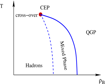
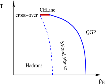
Figure 2: Left panel. A schematic picture of the deconfinement phase transition diagram in the plane of baryonic density $\rho_{B}$ and $T$ for the 2^nd order PT at the critical endpoint (CEP), i.e. for $\frac{3}{2}<\tau\leq 2$. For the 3^rd (or higher) order PT the boundary of the mixed and hadronic phases (dashed curve) should have the same slope as the boundary of the mixed phase and QGP (solid curve) at the CEP.
Right panel. Same as in the left panel, but for $\tau>2$. The critical endpoint in the $\mu_{B}-T$ plane generates the critical end line (CELine) in the $\rho_{B}-T$ plane shown by the thick horizontal line. This occurs because of the discontinuity of the partial derivatives of $s_{H}$ and $s_{Q}$ functions with respect to $\mu_{B}$ and $T$.

Assuming that the conditions (12) and (13) are fulfilled by the correct choice of the model parameters $B$ and ${\textstyle u(T,\mu_{B})}>0$, one can see now that at $T=T_{cep}$ there exists a PT as well, but its order is defined by the value of $\tau$. As was discussed in the preceding section for $\frac{3}{2}<\tau\leq 2$ there exists the 2^nd order PT. For $1<\tau\leq\frac{3}{2}$ there exist the PT of higher order, defined by the conditions formulated in Eq. (8). This is a new possibility, which, to my best knowledge, does not contradict to any general physical principle (see the left panel in Fig. 2).

The case $\tau>2$ can be ruled out because there must exist the first order PT for $T\geq T_{cep}$, whereas for $T<T_{cep}$ there exists the cross-over. Thus, the critical endpoint in $T-\mu_{B}$ plane will correspond to the critical interval in the temperature-baryonic density plane. Since such a structure of the phase diagram in the variables temperature-density has, to my knowledge, never been observed, I conclude that the case $\tau>2$ is unrealistic (see the right panel in Fig. 2). Note that a similar phase diagram exists in the FDM with the only difference that the boundary of the mixed and liquid phases (the latter in the QGBST model corresponds to QGP) is moved to infinite particle density.

4 Surface Tension Induced Phase Transition

Using our results for the case (III) of the preceding section, we conclude that above $T_{cep}$ there is a cross-over, i.e. the QGP and hadrons coexist together up to the infinite values of $T$ and/or $\mu_{B}$. Now, however, it is necessary to answer the question: How can the two different sets of singularities that exist on two sides of the line $T=T_{cep}$ provide the continuity of the solution of Eq. (3)?

It is easy to answer this question for $\mu_{B}<\mu_{B}^{c}(T_{cep})$ because in this case all partial $T$ derivatives of $s_{H}(T,\mu_{B})$, which is the rightmost singularity, exist and are finite at any point of the line $T=T_{cep}$. This can be seen from the fact that for the considered region of parameters $s_{H}(T,\mu_{B})$ is the rightmost singularity and, consequently, $s_{H}(T,\mu_{B})>s_{Q}(T,\mu_{B})$. The latter inequality provides the existence and finiteness of the volume integral in $F_{Q}(s,T,\mu_{B})$. In combination with the power $T$ dependence of the reduced surface tension coefficient $\sigma(T)$ the same inequality provides the existence and finiteness of all its partial $T$ derivatives of $F_{Q}(s,T,\mu_{B})$ regardless to the sign of $\sigma(T)$. Thus, using the Taylor expansion in powers of $(T-T_{cep})$ at any point of the interval $T=T_{cep}$ and $\mu_{B}<\mu_{B}^{c}(T_{cep})$, one can calculate $s_{H}(T,\mu_{B})$ for the values of $T>T_{cep}$ which are inside the convergency radius of the Taylor expansion.

The other situation is for $\mu_{B}\geq\mu_{B}^{c}(T_{cep})$ and $T>T_{cep}$, namely in this case above the deconfinement PT there must exist a weaker PT induced by the disappearance of the reduced surface tension coefficient. To demonstrate this we have solve Eq. (3) in the limit, when $T$ approaches the curve $T=T_{cep}$ from above, i.e. for $T\rightarrow T_{cep}+0$, and study the behavior of $T$ derivatives of the solution of Eq. (3) $s^{*}$ for fixed values of $\mu_{B}$. For this purpose we have to evaluate the integrals ${\cal K}_{\tau}(\Delta,\gamma^{2})$ introduced in Eq. (7). Here the notations $\Delta\equiv s^{*}-s_{Q}(T,\mu_{B})$ and $\gamma^{2}\equiv-\sigma(T)>0$ are introduced for convenience.

To avoid the unpleasant behavior for $\tau\leq 2$ it is convenient to transform (7) further on by integrating by parts:

$${\cal K}_{\tau}(\Delta,\gamma^{2})\,\equiv ~{}g_{\tau}(V_{0})-\frac{\Delta}{(\tau-1)}{\cal K}_{\tau-1}(\Delta,\gamma^{2})+\frac{\kappa\,\gamma^{2}}{(\tau-1)}{\cal K}_{\tau-\kappa}(\Delta,\gamma^{2})\,,$$ (15)

where the regular function $g_{\tau}(V_{0})$ is defined as

$$g_{\tau}(V_{0})\equiv\frac{1}{(\tau-1)\,V_{0}^{\tau-1}}\exp\left[-\Delta V_{0}+\gamma^{2}V_{0}^{\kappa}\right]\,.$$ (16)

For $\tau-a>1$ one can change the variable of integration $v\rightarrow z/\Delta$ and rewrite ${\cal K}_{\tau-a}(\Delta,\gamma^{2})$ as

$${\cal K}_{\tau-a}(\Delta,\gamma^{2}) = \Delta^{\tau-a-1}\int\limits_{V_{0}\Delta}^{\infty}dz~{}\frac{\exp\left[-z+\frac{\gamma^{2}}{\Delta^{\kappa}}z^{\kappa}\right]}{z^{\tau-a}}\equiv\Delta^{\tau-a-1}\,{\cal K}_{\tau-a}\left(1,\gamma^{2}\Delta^{-\kappa}\right)\,.$$ (17)

This result shows that in the limit $\gamma\rightarrow 0$, when the rightmost singularity must approach $s_{Q}(T,\mu_{B})$ from above, i.e. $\Delta\rightarrow 0^{+}$, the function (17) behaves as ${\cal K}_{\tau-a}(\Delta,\gamma^{2})\sim\Delta^{\tau-a-1}+O(\Delta^{\tau-a})$. This is so because for $\gamma\rightarrow 0$ the ratio $\gamma^{2}\Delta^{-\kappa}$ cannot go to infinity, otherwise the function ${\cal K}_{\tau-1}\left(1,\gamma^{2}\Delta^{-\kappa}\right)$, which enters into the right hand side of (15), would diverge exponentially and this makes impossible an existence of the solution of Eq. (3) for $T=T_{cep}$. The analysis shows that for $\gamma\rightarrow 0$ there exist two possibilities: either $\nu\equiv\gamma^{2}\Delta^{-\kappa}\rightarrow Const$ or $\nu\equiv\gamma^{2}\Delta^{-\kappa}\rightarrow 0$. The most straightforward way to analyze these possibilities for $\gamma\rightarrow 0$ is to assume the following behavior

$$\Delta=A\,\gamma^{\alpha}+O(\gamma^{\alpha+1})\,,~{}~{}\Rightarrow~{}~{}\frac{\partial\Delta}{\partial T}=\frac{\partial\gamma}{\partial T}\left[A\,\alpha\,\gamma^{\alpha-1}+O(\gamma^{\alpha})\right]\sim\frac{(2\,k+1)A\,\alpha\,\gamma^{\alpha}}{2\,(T-T_{cep})},$$ (18)

and find out the $\alpha$ value by equating the $T$ derivative of $\Delta$ with the $T$ derivative (5).

The analysis shows [3] that for $\Delta^{2-\tau}\leq\gamma\gamma^{\prime}\Delta^{1-\kappa}$ one finds

$$\gamma^{\alpha-2}\sim\Delta^{1-\kappa}\Rightarrow~{}\alpha\kappa=2~{}~{}{\rm for}~{}~{}\tau\leq 1+\frac{\kappa}{2k+1}\,.$$ (19)

Similarly, for $\Delta^{2-\tau}\geq\gamma\gamma^{\prime}\Delta^{1-\kappa}$ one obtains $\gamma^{\alpha-1}\gamma^{\prime}\sim\Delta^{2-\tau}$ and, consequently,

$$\alpha=\frac{2}{(\tau-1)(2k+1)}~{}~{}{\rm for}~{}~{}\tau\geq 1+\frac{\kappa}{2k+1}\,.$$ (20)

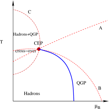
Figure 3: A schematic picture of the deconfinement phase transition diagram (full curve) in the plane of baryonic chemical potential $\mu_{B}$ and $T$ for the 2^nd order PT at the tricritical endpoint (CEP). The model predicts an existence of the surface induced PT of the 2^nd or higher order (depending on the model parameters). This PT starts at the CEP and goes to higher values of $T$ and/or $\mu_{B}$. Here it is shown by the dashed curve CEP-A, if the phase diagram is endless, or by the dashed-dot curve CEP-B, if the phase diagram ends at $T=0$, or by the dashed-double-dot curve CEP-C, if the phase diagram ends at $\mu_{B}=0$. Below (above) each of A or B curves the reduced surface tension coefficient is positive (negative). For the curve C the surface tension coefficient is positive outside of it.

Summarizing these results for $\gamma\rightarrow 0$, one can write the expression for the second derivative of $\Delta$ as [3]:

$$\frac{\partial^{2}\Delta}{\partial T^{2}}\sim\left\{\begin{tabular}[]{ll}\vspace{0.1cm} ${\textstyle\left[\frac{T-T_{cep}}{T_{cep}}\right]}^{\frac{2k+1}{\kappa}-2}$\,,& $\tau\leq 1+\frac{\kappa}{2k+1}$\,,\\ &\\ ${\textstyle\left[\frac{T-T_{cep}}{T_{cep}}\right]}^{\frac{3-2\tau}{\tau-1}}$\,,& $\tau\geq 1+\frac{\kappa}{2k+1}$\,.\end{tabular}\right.$$ (24)

The last result shows us that, depending on $\kappa$ and $k$ values, the second derivatives of $s*$ and $s_{Q}(T,\mu_{B})$ can differ from each other for $\frac{3}{2}<\tau<2$ or can be equal for $1<\tau\leq\frac{3}{2}$. In other words, it is found that at the line $T=T_{cep}$ there exists the 2^nd order PT for $\frac{3}{2}<\tau<2$ and the higher order PT for $1<\tau\leq\frac{3}{2}$, which separates the pure QGP phase from the region of a cross-over, i.e. the mixed states of hadronic and QGP bags. Since it exists at the line of a zero surface tension, this PT will be called the surface induced PT. For instance, from (24) it follows that for $k=0$ and $\kappa>\frac{1}{2}$ there is the 2^nd order PT, whereas for $k=0$ and $\kappa=\frac{1}{2}$ or for $k>0$ and $\kappa<1$ there is the 3^d order PT, and so on.

Since the analysis performed in the present section did not include any $\mu_{B}$ derivatives of $\Delta$, it remains valid for the $\mu_{B}$ dependence of the reduced surface tension coefficient, i.e. for $T_{cep}(\mu_{B})$. Only it is necessary to make a few comments on a possible location of the surface tension null line $T_{cep}(\mu_{B})$. In principle, such a null line can be located anywhere, if its location does not contradict to the sufficient conditions (12) and (13) of the 1^st deconfinement PT existence. Thus, the surface tension null line must cross the deconfinement line in the $\mu_{B}-T$ plane at a single point which is the tricritical endpoint $(\mu_{B}^{cep};T_{cep}(\mu_{B}^{cep}))$, whereas for $\mu_{B}>\mu_{B}^{cep}$ the null line should have higher temperature for the same $\mu_{B}$ than the deconfinement one, i.e. $T_{cep}(\mu_{B})>T_{c}(\mu_{B})$ (see Fig. 3). Clearly, there exist two distinct cases for the surface tension null line: either it is endless, or it ends at zero temperature or at other singularity, like the Color-Flavor-Locked phase. From the present lattice QCD data [32] it follows that the case C in Fig. 3 is the least possible.

To understand the meaning of the surface induced PT it is instructive to quantify the difference between phases by looking into the mean size of the bag:

$$\langle v\rangle\equiv-\frac{\partial\ln F(s,T,\mu_{B})}{\partial~{}~{}s}\biggl{|}_{s=s^{*}-0}\,.$$ (25)

As was shown in hadronic phase phase $\Delta>0$ and, hence, it consists of the bags of finite mean volumes, whereas, by construction, the QGP phase is a single infinite bag. For the cross-over states $\Delta>0$ and, therefore, they are the bags of finite mean volumes, which gradually increase, if the rightmost singularity approaches $s_{Q}(T,\mu_{B})$, i.e. at very large values $T$ and/or $\mu_{B}$. Such a classification is useful to distinguish QCD phases of present model: it shows that hadronic and cross-over states are separated from the QGP phase by the 1^st order deconfinement PT and by the 2^nd or higher order PT, respectively.

5 Concluding Remarks

Here I presented an analytically solvable statistical model which simultaneously describes the 1^st and 2^nd order PTs with a cross-over. The approach is general and can be used for more complicated parameterizations of the hadronic mass-volume spectrum, if in the vicinity of the deconfinement PT region the discrete and continuous parts of this spectrum can be expressed in the form of Eqs. (9) and (10), respectively. Also the actual parameterization of the QGP pressure $p=Ts_{Q}(T,\mu_{B})$ was not used so far, which means that our result can be extended to more complicated functions, that can contain other phase transformations (chiral PT, or the PT to color superconducting phase) provided that the sufficient conditions (12) and (13) for the deconfinement PT existence are satisfied.

In this model the desired properties of the deconfinement phase diagram are achieved by accounting for the temperature dependent surface tension of the quark-gluon bags. As was shown, it is crucial for the cross-over existence that at $T=T_{cep}$ the reduced surface tension coefficient vanishes and remains negative for temperatures above $T_{cep}$. Then the deconfinement $\mu_{B}-T$ phase diagram has the 1^st PT at $\mu_{B}>\mu^{c}_{B}(T_{cep})$ for $\frac{3}{2}<\tau<2$ , which degenerates into the 2^nd order PT (or higher order PT for $\frac{3}{2}\geq\tau>1$) at $\mu_{B}=\mu^{c}_{B}(T_{cep})$, and a cross-over for $0\leq\mu_{B}<\mu^{c}_{B}(T_{cep})$. These two ingredients drastically change the critical properties of the GBM [17] and resolve the long standing problem of a unified description of the 1^st and 2^nd order PTs and a cross-over, which, despite all claims, was not resolved in Ref. [34]. In addition, it was found that at the null line of the surface tension there must exist the surface induced PT of the 2^nd or higher order, which separates the pure QGP from the mixed states of hadrons and QGP bags, that coexist above the cross-over region (see Fig. 3). Thus, the QGBST model predicts that the QCD critical endpoint is the tricritical endpoint. It would be interesting to verify this prediction with the help of the lattice QCD analysis. For this one will need to study the behavior of the bulk and surface contributions to the free energy of the QGP bags and/or the string connecting the static quark-antiquark pair.

However, the QGP bags created in the experiments have finite mass, volume, life-time and, hence, the strong discontinuities which are typical for the 1^st order PT should be smeared out which would make them hardly distinguishable from the cross-over. Thus, to seriously discuss the signals of the 1^st order deconfinement PT and/or the tricritical endpoint, one needs to solve the finite volume version of the QGBST model like it was done for the SMM [11] and the GBM [12, 35]. This, however, is not sufficient because, in order to make any reliable prediction for experiments, the finite volume equation of state must be used in hydrodynamic equations which, unfortunately, are not suited for such a purpose. Thus, we are facing a necessity to return to the foundations of heavy ion phenomenology and to modify them according to the requirements of the experiments.

In addition, to apply the QGBST model to the experiments it is nesseary to make it more realistic: it seems that for the mixture of hadrons and QGP bags above the cross-over line it is necessary to include the relativistic treatment of hard core repulsion [36, 37] for lightest hardons and to include into statistical description the medium dependent width of hadronic resonances and QGP bags, which, as argued in Ref. [38], may completely change our understanding of the cross-over mechanism.

Acknowledgments. The author thanks V. K. Petrov for valuable comments. The research made in this work was supported by the Program “Fundamental Properties of Physical Systems under Extreme Conditions” of the Bureau of the Section of Physics and Astronomy of the National Academy of Science of Ukraine.

References

- [1] E. Farhi and R. L. Jaffe, Phys. Rev. D 30, 2379 (1984).
- [2] M. S. Berger and R. L. Jaffe, Phys. Rev. C 35, 213 (1987).
- [3] K. A. Bugaev, Phys. Rev. C 76, 014903 (2007).
- [4] L. G. Moretto, K. A. Bugaev, J. B. Elliott and L. Phair, nucl-th/0511180 15 p.
- [5] L. G. Moretto, L. Phair, K. A. Bugaev and J. B. Elliott, PoS CPOD2006:037 (2006) 18p.
- [6] M. E. Fisher, Physics 3, 255 (1967).
- [7] for a review on Fisher scaling see J. B. Elliott, K. A. Bugaev, L. G. Moretto and L. Phair, nucl-ex/0608022 (2006) 36 p. and references therein.
- [8] S. Das Gupta and A.Z. Mekjian, Phys. Rev. C 57, 1361 (1998).
- [9] K. A. Bugaev, M. I. Gorenstein, I. N. Mishustin and W. Greiner, Phys. Rev. C62, 044320 (2000); nucl-th/0007062 (2000); Phys. Lett. B 498, 144 (2001); nucl-th/0103075 (2001).
- [10] P. T. Reuter and K. A. Bugaev, Phys. Lett. B 517, 233 (2001).
- [11] K. A. Bugaev, Acta. Phys. Polon. B 36, 3083 (2005); and nucl-th/0507028, 7 p.
- [12] K. A. Bugaev, Phys. Part. Nucl. 38, 447 (2007).
- [13] L. Beaulieu et al., Phys. Lett. B 463, 159 (1999).
- [14] J. B. Elliott et al., (The EOS Collaboration), Phys. Rev. C 62, 064603 (2000).
- [15] K. A. Bugaev, L. Phair and J. B. Elliott, Phys. Rev. E 72, 047106 (2005).
- [16] K. A. Bugaev and J. B. Elliott, Ukr. J. Phys. 52, 301 (2007).
- [17] M. I. Gorenstein, V. K. Petrov and G. M. Zinovjev, Phys. Lett. B 106, 327 (1981).
- [18] R. Hagedorn, Nuovo Cimento Suppl. 3, 147 (1965).
- [19] L. G. Moretto, K. A. Bugaev, J. B. Elliott and L. Phair, Europhys. Lett. 76, 402 (2006).
- [20] K. A. Bugaev, J. B. Elliott, L. G. Moretto and L. Phair, hep-ph/0504011, 5p.
- [21] L. G. Moretto, K. A. Bugaev, J. B. Elliott and L. Phair, nucl-th/0601010, 4p.
- [22] D. G. Ravenhall, C. J. Pethick and J. R. Wilson, Phys. Rev. Lett. 50, 2066 (1983).
- [23] J. Liao and E. V. Shuryak, Phys. Rev. D 73, 014509 (2006).
- [24] I. Mardor and B. Svetitsky, Phys. Rev. D 44, 878 (1991).
- [25] G. Lana and B. Svetitsky, Phys. Lett. B 285, 251 (1992).
- [26] G. Neergaard and J. Madsen, Phys. Rev. D 62, 034005 (2000).
- [27] J. Ignatius, Phys. Lett. B 309, 252 (1993).
- [28] L. G. Moretto, K. A. Bugaev, J. B. Elliott, R. Ghetti, J. Helgesson and L. Phair, Phys. Rev. Lett. 94, 202701 (2005).
- [29] B. Krishnamachari et al. Phys. Rev. B 54, 8899 (1996).
- [30] R. D. Pisarski and F. Wilczek, Phys. Rev. D29, 338 (1984).
- [31] for qualitative arguments see M. Stephanov, Acta Phys. Polon. B 35, 2939 (2004).
- [32] F. Karsch and E. Laermann, in “Quark-Gluon Plasma 3”, edited by R. C. Hwa and X.-N. Wang (World Scientific, Singapore, 2004), p. 1 [hep-lat/0305025 ].
- [33] M. I. Gorenstein, G.M. Zinovjev, V.K. Petrov, and V.P. Shelest Teor. Mat. Fiz. (Russ) 52, 346 (1982).
- [34] M. I. Gorenstein, M. Gaździcki and W. Greiner, Phys. Rev. C 72, 024909 (2005).
- [35] K. A. Bugaev and P. T. Reuter, Ukr. J. Phys. 52, 489 (2007).
- [36] K. A. Bugaev, M. I. Gorenstein, H. Stöcker and W. Greiner, Phys. Lett. B 485, 121 (2000); G. Zeeb, K. A. Bugaev, P. T. Reuter and H. Stöcker, nucl-th/0209011, 16 p.
- [37] K. A. Bugaev, nucl-th/0611102., 18 p.
- [38] for a discussion and alternative cross-over mechanism see D. B. Blaschke and K. A. Bugaev, Fizika B 13, 491 (2004); Phys. Part. Nucl. Lett. 2, 305 (2005).