Power-law corrections to black-hole entropy via entanglement

Abstract

We consider the entanglement between quantum field degrees of freedom inside and outside the horizon as a plausible source of black-hole entropy. We examine possible deviations of black hole entropy from area proportionality. We show that while the area law holds when the field is in its ground state, a correction term proportional to a fractional power of area results when the field is in a superposition of ground and excited states. We compare our results with the other approaches in the literature.

1 Introduction

It is now well-known that the black-hole (commonly referred to as Bekenstein-Hawking) entropy is finite and is given by the relation [1]

$$S_{{}_{\rm BH}}=\frac{k_{B}}{4}\frac{A_{{}_{H}}}{\ell_{P}^{2}}\qquad{\rm where}\qquad\ell_{P}^{2}\equiv\frac{\hbar G}{c^{3}}\,,$$ (1)

$A_{{}_{H}}$ is the area of the black-hole horizon. It is infinite, if both the matter and gravity are purely classical! In other words, the finiteness of the black-hole entropy (and the validity of second-law of thermodynamics) requires that the matter and(or) gravity to be quantized.

Although the above relation has been derived by various approaches [2, 3, 4, 5], we do not yet understand: Why $S_{{}_{\rm BH}}$ is not extensive? What is the microscopic origin of black-hole entropy? Are there corrections to the Bekenstein-Hawking entropy? and How generic are these corrections?

The purpose of this paper is an attempt to understand the generic corrections to the Bekenstein-Hawking entropy by assuming entanglement as a source of black-hole entropy. We show that while the area law holds when the field is in its ground state, a correction term proportional to a fractional power of area results when the field is in a superposition of ground and excited states.

The paper is organized as follows: In the next section, we briefly discuss various properties of entanglement entropy and provide motivation for the relevance of the entanglement entropy to $S_{{}_{\rm BH}}$. In Sec. (3), we discuss the setup and the key steps in evaluating the entanglement entropy of scalar field propagating in flat space-time. In Sec. (4), we obtain the entanglement entropy for a superposed state and show explicitly that the power-law corrections become important for small horizon limit. We conclude with a summary in Sec. (5). In appendix, we show explicitly that at a fixed Lemaitre time, the Hamiltonian of a scalar field in a black hole background reduces to that in flat space-time.

2 Entanglement entropy

Let us consider a bipartite quantum system ${\mathcal{I}}\equiv\{12\}$ and assume that ${\mathcal{I}}$ is in a pure state $|\Psi\rangle$. The entanglement entropy ($S_{{}_{\rm ent}}$) is defined as

$$S_{{}_{\rm ent}}(\Psi)\equiv S(\rho_{1})=S(\rho_{2})$$ (2)

where

$$S(\rho_{1})=-Tr[\rho_{1}\ln(\rho_{1})]=-\sum_{n}p_{n}\ln p_{n}$$ (3)

is the Von Neumann entropy, $p_{n}$ are the Eigen-values of $\rho_{1}$ obtained by solving the integral equation

$$\int_{-\infty}^{\infty}dx^{\prime}\rho_{1}(x,x^{\prime})f_{n}(x^{\prime})=p_{n}f_{n}(x)$$ (4)

and

$$\rho_{1}=Tr_{2}(|\Phi\rangle\langle\Phi|)$$ (5)

is the reduced density matrix obtained by tracing over 2. Note that the entanglement entropy (2) is independent of the which degrees of freedom are traced over.

In order to set the ideas, we consider a simple example — 2-coupled harmonic oscillator. The Hamiltonian of a coupled Harmonic oscillator is given by

$$H=\frac{1}{2}\left[p_{1}^{2}+p_{2}^{2}+k_{0}\left(x_{1}^{2}+x_{2}^{2}\right)+k_{1}\left(x_{1}-x_{2}\right)^{2}\right]$$ (6)

where $(x_{i},p_{i})$ are coordinate and momenta of the oscillator, respectively, and $k_{1}$ is the interaction term which is assumed to be positive. The quantization of the above Hamiltonian is straight forward in the normal coordinates:

$$x_{\pm}=\frac{x_{1}\pm x_{2}}{\sqrt{2}}\,.$$ (7)

The ground state wave function is given by

$$\psi_{0}\left(x_{1},x_{2}\right)=\frac{\left(\omega_{+}\omega_{-}\right)^{1/4}}{\pi^{1/2}}\exp\left[-\left(\omega_{+}x_{+}^{2}+\omega_{-}x_{-}^{2}\right)/2\right]$$

where

$$\omega_{+}=\sqrt{k_{0}};~{}~{}\omega_{-}=\sqrt{k_{0}+2k_{1}};~{}~{}R^{2}=\frac{\omega_{+}}{\omega_{-}}<1\,.$$ (8)

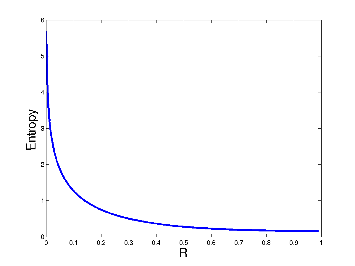
Figure 1: Plot of entanglement entropy of a coupled harmonic oscillator and $R$.

Let us consider the situation in which we choose not to have any information about the oscillator $1$. Mathematically, this corresponds to tracing over the oscillator 1, i. e.,

$$\rho_{2}\left(x_{2},x_{2}^{\prime}\right) = \int_{-\infty}^{\infty}dx_{1}\psi_{0}\left(x_{1},x_{2}\right)\psi_{0}^{\star}\left(x_{1},x_{2}^{\prime}\right)$$ (9)

$$= \sqrt{\frac{\gamma-\beta}{\pi}}\exp\left[-\frac{\gamma}{2}\left(x_{2}^{2}+x_{2}^{\prime 2}\right)+\beta x_{2}x_{2}^{\prime}\right]$$

where

$$\beta=\frac{\omega_{-}(1-R^{2})^{2}}{4(1+R^{2})};\quad\gamma=\omega_{-}\frac{1+6R^{2}+R^{4}}{4(1+R^{2})};\quad\xi=\left(\frac{1-R}{1+R}\right)^{2}<1\,.$$ (10)

Substituting (9) in the integral equation (4), the eigenfunctions and eigenvalues are given by

$$f_{n}(x)=H_{n}\left(\sqrt{\alpha}x\right)\exp\left(-\frac{\alpha x^{2}}{2}\right)\qquad p_{n}=\left(1-\xi\right)\xi^{n}~{}\,.$$ (11)

Substituting the eigenvalues in (3), the entanglement entropy is given by

$$S_{{}_{\rm ent}}(\xi)=-\ln(1-\xi)-\frac{\xi}{1-\xi}\ln(\xi)\,.$$ (12)

In Fig. (1), we have plotted $S_{{}_{\rm ent}}$ of the coupled oscillator in terms of $R$. It is interesting to note that the entanglement entropy vanishes when the oscillators are uncoupled ($R=1$) while they diverge in the strongly coupled limit ($R=0$).

But what has this digression to do with black-holes and what is the relevance of $S_{{}_{\rm ent}}$ to black-hole entropy? This can be understood from the fact that both entropies are associated with the existence of the horizons. Consider a scalar field on a background of a collapsing star. At early times, there is no horizon, and both the entropies are zero. However, once the horizon forms, $S_{{}_{\rm BH}}$ is non-zero, and if the scalar field degrees of freedom inside the horizon are traced over, $S_{{}_{\rm ent}}$ obtained from the reduced density matrix is non-zero as well.

In the next section, we give the procedure for evaluating the entanglement entropy of quantum scalar field propagating in flat space-time. In the Appendix, we have shown explicitly that at a fixed Lemaitre time, the Hamiltonian of a scalar field in Schwarzschild space-time reduces to that in flat space-time. All the results we derive in case of flat space-time can then be extended to the black-hole space-time at a fixed Lemaitre time.

3 Entanglement entropy for scalar fields – Setup

The Hamiltonian of a free massless scalar field propagating in the Minkowski space-time is given by

$$H=\frac{1}{2}\int d^{3}x\left[\pi^{2}(\vec{r})+|\nabla\varphi(\vec{r})|^{2}\right]\,.$$ (13)

For simplicity, let us assume that the scalar field in confined in a spherical box $\{12\}$. The cartoon version of the setup is provided in Fig (2).

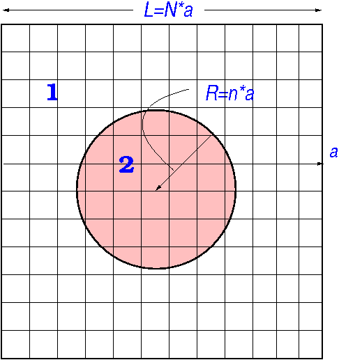
Figure 2: Sketch of the discretization of the scalar field propagating in the flat space-time. The shaded region is one we trace over.

Partial-wave decomposition of the scalar field and its canonical conjugate

$$\varphi_{lm}(r)=r\int d\Omega~{}Z_{lm}(\theta,\phi)\varphi(\vec{r});~{}~{}\pi_{lm}(r)=r\int d\Omega~{}Z_{lm}(\theta,\phi)\pi(\vec{r})$$ (14)

leads to the following reduced Hamiltonian:

$$H=\sum_{lm}H_{lm}=\sum_{lm}\frac{1}{2}\int_{0}^{\infty}\!\!\!\!dr\left[\pi_{lm}^{2}(r)+r^{2}\left[\frac{{\partial}}{{\partial}r}\left(\frac{\varphi_{lm}}{r}\right)\right]^{2}+\frac{l(l+1)}{r^{2}}\varphi_{lm}\right]\,,$$ (15)

where $Z_{lm}$ are the real Spherical harmonics. (For details, see Refs. [5, 6, 7].)

The computation of the entanglement entropy involves three steps: (i) Discretize the Hamiltonian, (ii) Choose a quantum state, and (iii) Trace over region 2 (or 1) to obtain the density matrix.

Note that, even if we obtain closed-form expression of the density matrix, it is not possible to analytically evaluate the entanglement entropy. Hence, we need to resort to numerical methods. In the rest of the section, we discuss these steps in detail.

3.1 Discretized Hamiltonian

Discretizing the Hamiltonian (15) in a spherical lattice as described in Fig. (2), we get

$$H_{lm} = \!\!\frac{1}{2a}\sum_{j=1}^{N}\left[\pi_{lm,j}^{2}+\left(j+\frac{1}{2}\right)^{2}\left(\frac{\varphi_{lm,j}}{j}-\frac{\varphi_{lm,j+1}}{j+1}\right)^{2}\right.+\left.\frac{l(l+1)}{j^{2}}~{}\varphi_{lm,j}^{2}\right]$$ (16)

$$= \frac{1}{2a}\sum_{j=1}^{N}\pi_{j}^{2}+\frac{1}{2a}\sum_{i,j=1}^{N}\varphi_{i}K_{ij}\varphi_{j}\,,$$

where $a$ is the lattice spacing, $L$ ($\gg a$) is the length of the box, $N$ is the number of lattice points and the interaction matrix $K_{ij}$ is given by

$$\!\!\!\!\!\!\!\!K_{ij} = \frac{1}{i^{2}}\left[\left(i+\frac{1}{2}\right)^{2}+\left(i-\frac{1}{2}\right)^{2}\right]\delta_{i,j(i\neq 1,N)}$$

$${\frac{1}{i^{2}}\left[l(l+1)+\frac{9}{4}~{}\delta_{i1}\delta_{j1}+\left[N-\frac{1}{2}\right]^{2}\delta_{iN}\delta_{jN}\right]}$$

$$\underbrace{{\color[rgb]{0,0,1}-\left[\frac{(j+\frac{1}{2})^{2}}{j(j+1)}\right]\delta_{i,j+1}-\left[\frac{(i+\frac{1}{2})^{2}}{i(i+1)}\right]\delta_{i,j-1}}}_{{\color[rgb]{0,0,0}\mbox{nearest neighbor interaction}}}$$

$${K}=\left(\begin{array}[]{lllllll}{\times}&{\color[rgb]{0,0,1}\times}&{}&{}&{}&{}&{}\\ {\color[rgb]{0,0,1}\times}&{\times}&{\color[rgb]{0,0,1}\times}&{}&{}&{}&{}\\ {}&{\color[rgb]{0,0,1}\times}&{\times}&{\color[rgb]{0,0,1}\times}&{}&{}&{}\\ {}&{}&{\color[rgb]{0,0,1}\times}&{\times}&{\color[rgb]{0,0,1}\times}&{}&{}\\ {}&{}&{}&{\color[rgb]{0,0,1}\times}&{\times}&{\color[rgb]{0,0,1}\times}&{}\\ {}&{}&{}&{}&{\color[rgb]{0,0,1}\times}&{\times}&{\color[rgb]{0,0,1}\times}\\ {}&{}&{}&{}&{}&{\color[rgb]{0,0,1}\times}&{\times}\\[8.0pt] \end{array}\right)$$

Note that the Hamiltonian (16) is a $N$-coupled Harmonic oscillators which satisfy the following commutation relations:

$$[\varphi_{lm,j},\pi_{l^{\prime}m^{\prime},j^{\prime}}]=i\delta_{ll^{\prime}}\delta{mm^{\prime}}\delta{jj^{\prime}}$$ (24)

3.2 Choice of quantum state

The general Eigen state of the $N$-coupled harmonic oscillators is

$$\Psi(x_{1},\dots,x_{n},x_{n+1},\dots,x_{N})=\left[\frac{|\Omega|}{\pi^{N}}\right]^{1/4}~{}\exp\left[-\frac{x^{T}\cdot\Omega\cdot x}{2}\right]\times\prod_{i=1}^{N}\frac{1}{\sqrt{2^{\nu_{i}}\nu_{i}}}~{}H_{\nu_{i}}\left({K_{D}^{\frac{1}{4}}}_{i}~{}\bar{x}_{i}\right)$$

where $K_{D}$ is the diagonal matrix of $K$ obtained by the unitary transformation $K=U^{T}K_{D}U$, $U$ is a unitary matrix and $\Omega=U^{T}K_{D}^{1/2}U$.

It is not possible to obtain a closed form expression for the density matrix for such a general state. To make the calculations tractable, we make two choices for the $N$-particle state:

1. Vacuum state: In this case, the $N$-particle wave function is given by [4] (see also [9, 10])

   $$\Psi_{0}(x_{1},\dots,x_{n},x_{n+1},\dots,x_{N})=\left[\frac{|\Omega|}{\pi^{N}}\right]^{1/4}\exp\left[-\frac{x^{T}\cdot\Omega\cdot x}{2}\right]$$ (25)

2. 1-particle state: In this case, the $N$-particle wave function is given by [5]

   $$\Psi_{{}_{1}}(x_{1}\dots x_{N}) = \left|\frac{\Omega}{4\pi^{N}}\right|^{\frac{1}{4}}\sum_{i=1}^{N}a_{i}H_{1}\left(k_{Di}^{\frac{1}{4}}{x}_{i}\right)\exp\left[-\frac{1}{2}k_{Di}^{\frac{1}{2}}~{}{x}_{i}^{2}\right]$$ (26)

   $$\sqrt{2}~{}\left(a^{T}K_{D}^{\frac{1}{2}}{x}\right)~{}\psi_{0}\left(x_{1},\dots,x_{N}\right)$$

   where $a\mbox{'s are expansion coefficients}$ which satisfy the condition $a^{T}a=1$. For detailed discussion see [5, 6].

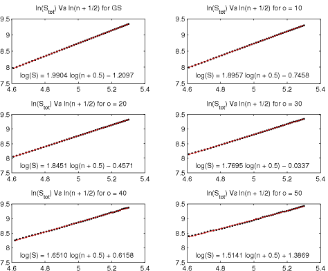
Figure 3: The entanglement entropy for ground and 1-Particle states for $N=300,n=100-200,o=10-50$

3.3 Density matrix

For a general Eigen state, the physical operation of trace over region 2 ($n<N$ oscillators) [cf. Fig. (2)] is given by

$$\rho_{n}\left(x_{n+1}\cdots x_{N};x^{\prime}_{n+1}\cdots x_{N}\right) = \int\prod_{i=1}^{n}~{}dx_{i}~{}\Psi(x_{1}\dots x_{N})\Psi^{\star}(x_{1}\dots x_{n};x^{\prime}_{n+1}\cdots x^{\prime}_{N})$$

For the two special choices which we discussed in the previous subsection, the above expression reduces to

1. Vacuum state:

   $$\rho_{{}_{GS}}=\prod_{i=1}^{n}~{}\rho_{2}(z_{i},z_{i}^{\prime})$$ (27)

   which corresponds to product of $n$ 2-coupled harmonic oscillators with 1 harmonic oscillator traced as discussed in Sec. (2).

2. 1-Particle state:

   $$\rho_{{}_{ES}}=\rho_{{}_{GS}}Tr(\Lambda_{A}A^{-1})\left[1-\frac{1}{2}\left(t^{T}\Lambda_{\gamma}t+t^{\prime T}\Lambda_{\gamma}t^{\prime}\right)+t^{T}\Lambda_{\beta}t^{\prime}\right]\,,$$

   where

   $$\Lambda=U^{T}~{}K_{D}^{\frac{1}{4}}~{}a~{}a^{T}~{}K_{D}^{\frac{1}{4}}~{}U\equiv\left(\begin{array}[]{cc}\Lambda_{A}&\Lambda_{B}\\ \Lambda_{B}^{T}&\Lambda_{C}\end{array}\right)~{};\Omega=U^{T}K_{D}^{1/2}U\equiv\left(\begin{array}[]{cc}A&B\\ B^{T}&C\end{array}\right)~{};$$ (32)

   $$t\equiv(t_{1},\cdots t_{N-n})=(\varphi_{n}\cdots\varphi_{N})$$

   $$\Lambda_{\gamma}=\frac{2\Lambda_{B}^{T}\left(A^{-1}B\right)-B^{T}\left(A^{-1}\right)^{T}\Lambda_{A}A^{-1}B}{Tr(\Lambda_{A}A^{-1})}$$

   $$\Lambda_{\beta}=\frac{2\Lambda_{{}_{C}}+B^{T}\left[A^{-1}\right]^{T}\!\Lambda_{{}_{A}}A^{-1}B-\Lambda_{{}_{B}}^{T}A^{-1}B-B^{T}\!\left[A^{-1}\right]^{T}\!\Lambda_{{}_{B}}}{Tr(\Lambda_{{}_{A}}A^{-1})}$$ (33)

As mentioned earlier, it is not possible to evaluate the entanglement entropy analytically and we need to resort to numerical computations. We use Matlab to evaluate the entropy and the numerical error in our computation is less than $0.1\%$.

In Fig. (3), we have plotted the entanglement entropy for the ground state and 1-particle state for $N=300,n=100-200,o=10-50$. We see that for the 1-particle state, the entropy scales as ${\mathcal{A}}^{\mu}$, with lesser $\mu$ for higher $o$. It is less than unity for any $o>0$ i. e., more the excitation, larger is deviation from area law The area law does not seem to hold! This implies that the entanglement entropy depends on the choice of the quantum state of the field.

4 Power law corrections to area

Given the above results, one may draw two distinct conclusions: first that entanglement entropy is not robust and reject it as a possible source of black-hole entropy. Second, since entanglement entropy for excited state scales as a lower power of area it is plausible that when a generic state (consisting of a superposition of ground state and excited state) is considered, corrections to the Bekenstein-Hawking entropy will emerge. In order to determine which one is correct, it is imperative to investigate various generalizations of the scenarios considered in Ref. [5]. To this end, in this section we calculate the entanglement entropy of the mixed superposition of vacuum and 1-particle state

$$\Psi=c_{0}\Psi_{0}+c_{1}\Psi_{1}\qquad{\rm where}\qquad{|c_{0}|^{2}+|c_{1}|^{2}=1}\,.$$ (34)

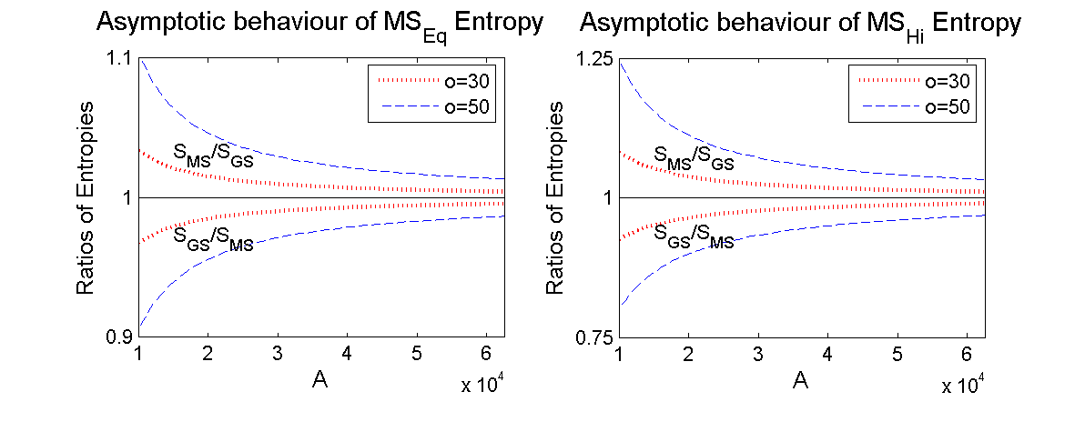
Figure 4: Plots of the relative entropy with the area for $N=300,n=100-200$ and $o-30,50$ where (i) $MS_{EQ}$ corresponds to $|c_{0}|=|c_{1}|=0.7$ and (ii) $MS_{Hi}$ corresponds to $|c_{0}|=0.5$, $|c_{1}|=0.87$.

Following the procedure discussed in the previous section, it is possible to obtain the entanglement entropy of the superposed state. In Fig. (4) we have plotted the relative entropy [i.e ratio of the superposed and ground state entanglement entropy] for different values of $c_{0}$ and $c_{1}$. From Fig. (4) it is easy to see that for large values of the horizon radius the entanglement entropy of the superposed state approaches the ground state entanglement entropy. In other words, for large horizon area, the entanglement entropy of the superposed state scales as area of the horizon.

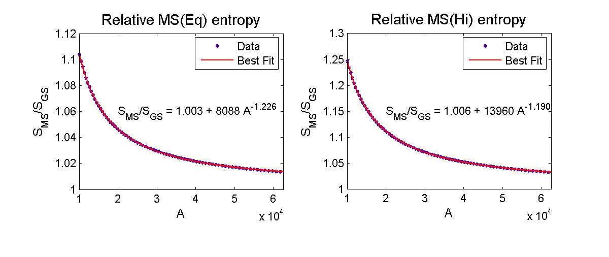
Figure 5: The best fit the relative entropy vs ${\mathcal{A}}$ for (i) $MS_{EQ}$ corresponds to $|c_{0}|=|c_{1}|=0.7$ and (ii) $MS_{Hi}$ corresponds to $|c_{0}|=0.5$, $|c_{1}|=0.87$

In order to know the behavior of the entanglement entropy for the small horizon limit, in Fig. (5), we have obtained the best numerical fit for the relative entropy. From these, we see that the entanglement entropy of the superposed state is given by:

$$S=c_{1}\,{\mathcal{A}}\,\left(1+\frac{c_{2}}{{\mathcal{A}}^{\beta}}\right)$$ (35)

where $\beta>0$ and $c_{1},c_{2}$ are constants. This is the main result of this paper and we would like to stress the following points: (i) The second term in the above expression may be regarded as a power law correction to the area law, resulting from entanglement, when the wave-function of the field is chosen to be a superposition of ground and excited states. (ii) It is important to note that the correction term falls off rapidly with ${\mathcal{A}}$ (due to the negative exponent) and in the large area limit (${\mathcal{A}}\gg 1$) the area-law is recovered. This lends further credence to entanglement as a possible source of black hole entropy. (iii) The correction term is more significant for greater excited state-ground state mixing proportion $c_{1}$. For detailed discussion see Refs. [7, 8].

5 Conclusions

In this work, we have obtained power-law corrections to the Bekenstein-Hawking entropy, treating the entanglement between scalar field degrees of freedom inside and outside the horizon as a viable source of black-hole entropy. We have shown that for small black hole areas the area law is violated when the oscillator modes are in a linear superposition of ground and excited states. We found that the corrections to the area-law become increasingly significant as the proportion of excited states in the superposed state increases. Conversely, for large horizon areas, these corrections are relatively small and the area-law is recovered.

Power law corrections to the Bekenstein- Hawking entropy has been encountered earlier in other approaches to black hole entropy. For instance, the Noether charge approach predicts a generic power law correction to the Bekenstein-Hawking entropy [11]. For instance, using Noether charge as entropy, it was shown for 5-dimensional Gauss-Bonnet gravity

$${\mathcal{S}}_{GB}^{5D}=\frac{1}{16\pi G}\int d^{5}x\sqrt{-g}\left[R+\alpha_{GB}\left(R^{2}-4R_{ab}R^{ab}+R_{abcd}R^{abcd}\right)\right]\quad\alpha_{GB}\mbox{~{}is a constant}\,,$$ (36)

that the entropy corresponding to a Killing horizon is [12]

$$S_{{}_{\rm NC}}^{5D}=\frac{A}{4}\left(1+\frac{c_{3}}{A^{2/3}}\right)\,.$$ (37)

Although both these approaches lead to power-law corrections, there are couple of crucial differences between the two: (i) In the case of Noether charge, the power-law corrections to the Bekenstein-Hawking entropy arises due to the higher-derivative terms in the gravity action. However, the corrections we have derived is also valid for Einstein-Hilbert action. (ii) The Noether charge entropy does not identify which degrees of freedom contribute most to the entropy. In our case, we have shown that the maximum entropy contribution for the area-law come close to the horizon while significant contribution to the power-law corrections arise from the degrees of freedom far from the horizon [7, 8].

SS is supported by the Marie Curie Incoming International Grant IIF-2006-039205.

Appendix A Scalar fields in Schwarzschild space-time

In this section, we generalize the framework of our calculations, so that they are applicable to black hole space-times. We start with the Schwarzschild metric with a horizon at $r=r_{0}$:

$$ds^{2}=-f(r)dt^{2}+\frac{dr}{f(r)}+r^{2}d\Omega^{2}~{},~{}~{}f(r)=1-\frac{r_{0}}{r}$$ (38)

and define the following coordinate transformation from $(t,r)$ to $(\tau,R)$ coordinates:

$$\tau=t+r_{0}\left[\ln\left(\frac{1-\sqrt{r/r_{0}}}{1+\sqrt{r/r_{0}}}\right)+2\sqrt{\frac{r}{r_{0}}}\right]~{},~{}R=\tau+\frac{2~{}r^{\frac{3}{2}}}{3\sqrt{r_{0}}}~{},~{}r=\left[\frac{3}{2}\left(R-\tau\right)\right]^{\frac{2}{3}}r_{0}^{\frac{1}{3}}~{},$$ (39)

such that (38) transforms to the following metric, in Lemaitre coordinates:

$$ds^{2}=-d\tau^{2}+\frac{dR^{2}}{\left[\frac{3}{2r_{0}}\left(R-\tau\right)\right]^{\frac{2}{3}}}+\left[\frac{3}{2r_{0}}\left(R-\tau\right)\right]^{\frac{4}{3}}r_{0}^{\frac{2}{3}}~{}d\Omega^{2}~{}.$$ (40)

The Hamiltonian for a free scalar field in the above space-time can be written as :

$$H(\tau)=\frac{1}{2}\int_{\tau}^{\infty}dR\left[\frac{2\pi(\tau,R)^{2}}{3(R-\tau)}+\frac{3}{2}~{}r~{}(R-\tau)\left({\partial}_{R}\phi(\tau,R)\right)^{2}\right]~{}.$$ (41)

Next, choose a fixed Lemaitre time, say $\tau=0$ and perform the following field redefinitions:

$$\pi(r)=\sqrt{r}\pi_{1}(r)~{},~{}~{}\phi(r)=\frac{\phi_{1}(r)}{r}~{}.$$ (42)

Then, at that fixed time, the Hamiltonian (41) transforms to:

$$H(0)=\frac{1}{2}\int_{0}^{\infty}dr\left[\pi_{1}(r)^{2}+r^{2}\left({\partial}_{r}\frac{\phi_{1}}{r}\right)^{2}\right]~{}.$$ (43)

Note that this is identical to the Hamiltonian in flat space-time, Eq.(13). Hence, all the analysis in Secs. (2,3) will go through for a black-hole space-time in a fixed Lemaitre time.

References

References

• [1] J. D. Bekenstein, Phys. Rev.  D 7, 2333 (1973); Phys. Rev.  D 9, 3292 (1974); Phys. Rev.  D 12, 3077 (1975). S. W. Hawking, Nature 248, 30 (1974).
• [2] A. Strominger, C. Vafa, Phys. Lett. B379, 99 (1996); A. Ashtekar et al, Phys. Rev. Lett. 80, 904 (1998); S. Carlip, ibid 88, 241301 (2002); A. Dasgupta, Class. Quant. Grav. 23, 635 (2006).
• [3] L. Bombelli, R. K. Koul, J. H. Lee and R. D. Sorkin, Phys. Rev.  D 34, 373 (1986).
• [4] M. Srednicki, Phys. Rev. Lett.  71, 666 (1993) [arXiv:hep-th/9303048].
• [5] S. Das and S. Shankaranarayanan, Phys. Rev.  D 73, 121701 (2006) [arXiv:gr-qc/0511066].
• [6] S. Das and S. Shankaranarayanan, J. Phys. Conf. Ser.  68, 012015 (2007) [arXiv:gr-qc/0610022].
• [7] S. Das and S. Shankaranarayanan, Class. Quant. Grav. 24, 5299 (2007) [arXiv:gr-qc/0703082].
• [8] S. Das, S. Shankaranarayanan and S. Sur, arXiv:0705.2070 [gr-qc].
• [9] M. B. Plenio, J. Eisert, J. Dreissig and M. Cramer, “Entropy, entanglement, and area: analytical results for harmonic lattice Phys. Rev. Lett.  94, 060503 (2005); [arXiv:quant-ph/0405142]. M. Cramer, J. Eisert, M. B. Plenio and J. Dreissig, Phys. Rev.  A 73, 012309 (2006) [arXiv:quant-ph/0505092].
• [10] A. Yarom and R. Brustein, Nucl. Phys.  B 709, 391 (2005) [arXiv:hep-th/0401081]; R. Brustein, M. B. Einhorn and A. Yarom, JHEP 0601, 098 (2006) [arXiv:hep-th/0508217].
• [11] R. M. Wald, Phys. Rev.  D 48, 3427 (1993) [arXiv:gr-qc/9307038].
• [12] R. C. Myers and J. Z. Simon, Phys. Rev.  D 38, 2434 (1988).