AMI limits on 15 GHz excess emission in northern Hii regions

Abstract

We present observations between 14.2 and 17.9 GHz of sixteen Galactic Hii regions made with the Arcminute Microkelvin Imager (AMI). In conjunction with data from the literature at lower radio frequencies we investigate the possibility of a spinning dust component in the spectra of these objects. We conclude that there is no significant evidence for spinning dust towards these sources and measure an average spectral index of $\alpha=0.15\pm 0.07$ (where $S\propto\nu^{-\alpha}$) between 1.4 and 17.9 GHz for the sample.

1 Introduction

Recent observations of Galactic targets (Finkbeiner et al. 2002; 2004; Casassus et al. 2004;2006; Watson et al. 2005; Scaife et al. 2006; Dickinson et al. 2007) have provided some evidence for the anomalous microwave emission commonly ascribed to spinning dust (Drain & Lazarian 1998a,b). This emission was first seen as a large scale phenomenon in CMB observations and represented a problem as it emits in the frequency range   10–60 GHz (Kogut et al. 1996; Leitch et al. 1997; de Oliviera-Costa et al. 2002; 2004) close to the minimum of the combined synchrotron, Bremsstrahlung and thermal dust emissions at 70 GHz. Indeed the models of Draine & Lazarian predict a spectrum for spinning dust which is strongly peaked between 20 and 40 GHz. Arising as a consequence of rapidly rotating small dust grains the emission has been suggested to occur in a number of distinct astronomical objects and to be highly correlated with thermal dust emission; this has been supported by some of the pointed observations referred to earlier and by recent evidence of diffuse emission at medium to high galactic latitudes from correlations made with WMAP data (Davies et al. 2006).

Previous observations of Hii regions in the microwave region of the spectrum have shown evidence both for (Watson et al. 2005; Dickinson et al. 2007) and against (Dickinson et al. 2006; Scaife et al. 2007) the presence of a spinning dust component in the emission of these objects. Since the behaviour of Hii regions at radio frequencies is relatively well understood they provide an excellent testing ground for examining this phenomenon. At frequencies below $\sim$100 GHz Hii regions are expected to be dominated by free-free emission, or thermal Bremsstrahlung. This mechanism progresses from the optically thick regime to the optically thin at around 1 GHz, and possesses a characteristically shallow spectrum ($\alpha=0.1$; where $S\propto\nu^{-\alpha}$) at frequencies above this turn over.

Here we present observations of sixteen Galactic Hii regions selected from the VLA survey of optically visible Galactic Hii regions (Fich 1993). Using spectral data from the AMI in conjunction with measurements from the literature we model the spectrum of free-free radiation and compare it with our own measurements in order to place limits on possible excess emission at 15 GHz, which may arise from spinning dust. We use the correlated FIR (100, 60, 25 and 12 $\mu$m) emission to further constrain this excess.

2 The Telescope

The Arcminute Microkelvin Imager (AMI) is located at the Mullard Radio Astronomy Observatory, Lord’s Bridge, Cambridge, UK. Its Small Array is composed of ten 3.7 m diameter equatorially mounted dishes with a baseline range of $\sim$5 to 20 m. The telescope observes in the band 12–18 GHz with cryostatically cooled NRAO indium-phosphide front-end amplifiers. The system temperature is typically about 25 K. The astronomical signal is mixed with a 24 GHz oscillating signal to produce an IF signal of 6–12 GHz. The correlator is an analogue Fourier transform spectrometer with 16 correlations formed for each baseline at path delays spaced by 25 mm. Both in phase and out of phase correlations are performed. From these, eight channels of 750 MHz bandwidth are synthesised. The AMI Small Array is sensitive to angular scales of $\sim 1^{\prime}$ to $\sim 15^{\prime}$ and has a primary beam FWHM of $\approx 20^{\prime}$ at 15 GHz. The lowest two channels are generally unused due to a low response in this frequency range, and strong interference from European geostationary satellites.

3 Observations

Observations of sixteen Hii regions, see Table 1, were made with the AMI Small Array during the period May–June 2007. These targets were selected from the VLA survey of optically visible Galactic Hii regions (Fich 1993) on the basis of flux density, angular diameter and declination. The sample, see Table 1, was divided on the basis of flux at 4.89 GHz. The positions and effective thermal noise associated with each AMI observation are shown in Table 1. Observations were typically 8 hours long and used interleaved calibration on bright point sources at hourly intervals for phase calibration. The sensitivity of AMI is $\approx$30 mJy s^-1/2 giving $\approx$0.2 mJy after 8 hours observation. Given that the objects observed here are bright, eight hours is more than sufficient to obtain accurate fluxes; however the long observations are important to produce good maps, the structure of which is dependent on the uv-coverage.

Table 1: AMI Hii region sample. Names of the form S$nnn$ are taken from the Sharpless (1959) catalogue of Hii regions; and names of the form BFS$nn$ are taken from the catalogue of Blitz, Fich & Stark (1982). Radio positions are adapted from Fich (1993). Column 4 contains the effective thermal noise for the AMI observation of each object.

Name	$\alpha^{1}$	$\delta$	$\sigma_{\rm{th}}$
	(J2000)	(J2000)	(mJy)
$S_{4.89}$ $\geq$ 1 Jy:
S100	20 01 44.7	+33 31 14	7.760
S152	22 58 40.8	+58 47 02	1.099
$S_{4.89}$ $\geq$ 0.5 Jy:
S127	21 28 38.0	+54 35 12	0.710
S138	22 32 45.2	+58 28 21	0.629
S149	22 56 17.4	+58 31 18	0.593
S211	04 36 57.0	+50 52 36	0.646
S288	07 08 37.0	-04 18 48	3.703
$S_{4.89}$ $\geq$ 0.1 Jy:
S121	21 05 15.8	+49 40 06	0.650
S167	23 35 30.9	+64 52 28	0.330
S175	00 27 17.0	+64 42 23	0.319
S186	01 08 50.5	+63 07 34	1.033
S256	06 12 36.0	+17 56 54	1.288
S259	06 11 25.8	+17 26 25	0.537
S271	06 14 59.4	+12 20 16	0.652
BFS10	21 56 30.4	+58 01 43	0.501
BFS46	05 40 52.9	+35 42 17	0.727

¹ positions adapted from Fich (1993)

Table 2: Assumed fluxes of 3C286 and 3C48 over the AMI bandwidth.

Channel	$\bar{\nu}$	$S^{\rm{3C286}}$/Jy	$S^{\rm{3C48}}$/Jy
1	12.788	3.909	1.941
2	13.512	3.755	1.832
3	14.235	3.614	1.734
4	14.958	3.485	1.646
5	15.682	3.366	1.566
6	16.405	3.257	1.494
7	17.128	3.155	1.428
8	17.852	3.061	1.367

Table 3: Phase calibrators used during Hii region observations. 8 GHz flux densities are from JVAS; 15 GHz flux densities are from the VLA Calibration Source List¹ and from the AMI Hii region sample described in this work. If a source is known to variable it is indicated.

Source	$\alpha$(J2000)	$\delta$(J2000)	$S_{8}$(Jy)	$S_{15}^{\rm{VLA}}$(Jy)	$S_{15}^{\rm{AMI}}$(Jy)	variable?	Hii Regions calibrated
J0100+681	01 00 51.7	+68 08 21	0.856	0.6	0.610	no	S167, S175
J0102+584	01 02 45.8	+58 24 11	1.399	2.3	3.070	yes	S186
J0359+509	03 59 29.7	+50 57 50.2	2.404	10.5	9.280	yes	S211
J0539+1433	05 39 42.4	+14 33 46	1.093	0.5	0.660	yes	S256, S259, S271
J0555+398	05 55 30.8	+39 48 49	6.984	2.8	3.560	yes	BFS46
J0739+0137	07 39 18.0	+01 37 05	1.746	2.1	2.430	yes	S288
J2025+3343	20 25 10.8	+33 43 00	2.592	2.5	2.410	yes	S100
J2038+513	20 38 37.0	+51 19 13	4.205	3.3	3.140	yes	S121
J2125+643	21 25 27.4	+64 23 39	1.127	0.6	0.570	no	BFS10
J2201+508	22 01 43.5	+50 48 56	0.815	0.6	0.300	yes	S127
J2322+509	23 22 26.0	+50 57 52	1.656	1.6	0.940	yes	S152, S138, S149

¹Version (08/2002): http://www.nrao.edu/$\sim$gtaylor/calib.html

4 Calibration and Data reduction

Data reduction was performed using the local software tool reduce, developed from the VSA data-reduction software of the same name. This applies appropriate path compensator and path delay corrections, flags interference, shadowing and hardware errors, applies phase and flux calibrations and Fourier transforms the data into uv fits format suitable for imaging in aips.

Flux calibration was performed using short observations of 3C48 and 3C286 near the beginning and end of each run; assumed flux densities for these sources in the AMI channels as taken from Baars et al. (1977) are shown in Table. 2. In addition to the flux calibration each observation was interleaved with a secondary phase calibrator.

Secondary calibrators are selected from the Jodrell Bank VLA Survey (hereinafter JVAS; Patnaik et al. 1992; Browne et al. 1998; Wilkinson et al. 1998) on the basis of their declination and flux. A list of these calibrators is given in Table 3. Over one hour the phase is generally stable to $5^{\circ}$ for Channels 4–7, and $10^{\circ}$ for Channels 3 and 8.

A weather correction is also made using data from the ‘rain gauge’. This measures the sky temperature in correlator units which are calibrated by measuring the rain gauge response on a cool, dry, clear day. From cross-calibration of our primary calibrators we find that the weather correction and primary calibration give fluxes correct within 5 per cent.

Low declination observations can be highly contaminated by geostationary satellites. Much of this emission is in the low frequency channels, which are usually discarded. However narrow-band emission at 15 GHz can seriously contaminate astronomical data. As the satellites are fixed against the moving astronomical sky, a high-pass filter applied to the phase centre before fringe rotation can remove the bulk of the contamination, although this results in the loss of all low-v visibilities in the uv-plane.

5 Imaging and Spectra

Reduced data were imaged using the aips data package. Maps were made from both the combined channel set, shown in this paper, and from individual channels. The broad spectral coverage of the AMI allows a representation of the spectrum between 14 and 18 GHz to be made. Errors on the AMI data points were calculated using a 5 per cent error on the flux and the thermal noise of each individual observation as calculated from the data. This error of 5 per cent on the flux of each source is a conservative error on the day-to-day calibration of the telescope which has been found to be significantly better than 5 per cent. It also includes a contribution for the Gaussian fitting of the sources although in most cases this fitting was found to be robust to changes in fitting area, a test which usually reveals cases where the source is poorly fitted. The overall error was calculated as $\sigma=\sqrt{(\sigma_{\rm{th}}^{2}+(0.05S_{\rm{i}})^{2})}$, where $\sigma_{\rm{th}}$ is the thermal noise calculated outside the primary beam for that observation and $S_{\rm{i}}$ is the integrated flux density of the source. For those observations heavily contaminated by satellite interference a more conservative 10 per cent error is placed on the flux density calibration. The central frequency of channels 3–8 is 15.8 GHz and fluxes from the combined channels can be found in Table 5.

In the Northern sky a number of Galactic surveys exist. At 1.4 GHz, measurements from the Effelsberg telescope (Reich et al. 1997) and from the NVSS (Condon et al. 1998) can be compared, with due caution employed considering the relative angular resolution and inherent flux losses from the VLA compared with the Effelsberg 100 m dish. In addition to these the Canadian Galactic Plane Survey (hereinafter CGPS) provides pseudo total power observations of the Galactic plane at 1.4 GHz by combining single dish and interferometer data to achieve a resolution of 1 arcmin. At 2.7 GHz the Effelsberg Galactic plane survey (Fürst et al. 1990a;b)is available, and the low latitude Galactic survey from the Parkes observatory (Day et al. 1972) also covers a small number of our low declination sources. At higher frequencies the GB6 survey (Gregory et al. 1996) at 4.85 GHz and the Galactic plane survey of Langston et al (2000) at 8.35 and 14.35 GHz can be used, although the detection limit of 0.9 Jy at 8.35 GHz and 2.5 Jy at 14.35 GHz restricts these measurements to only the brightest sources.

In addition to these surveys a number of pointed Hii samples have been made including those of Gregory and Taylor (1986) at 5 GHz, Kallas & Reich (1980); Kazes, Walmsley & Churchwell (1977) again with the Effelsberg 100 m dish, Felli (1978) at 6 arcsecond resolution using the Westerbork telescope and a number of small samples of Hii regions were presented in a series of papers (Israel, Habing & de Jong 1973; Israel 1976a,b; 1977a,b,c).

6 Results

Gaussian fits were made to the sources found in the AMI images, allowing for a background component. The integrated flux of each source was then used in conjunction with fluxes from the literature to constrain the radio spectrum of each object. Since the bandwidth of AMI stretches from 14.2 GHz to 17.9 GHz it is possible to constrain the microwave spectrum of each Hii region independently of other measurements. However, to investigate the spectral behaviour of these objects through the radio and into the microwave regime we also combine our own fluxes with those from other catalogues. We include data from the NVSS catalogue at 1.4 GHz and also from the VLA survey of optically identified Hii regions from which our sample is taken. The second of these catalogues has measurements at 4.89 GHz, and occasionally 1.42 GHz. Since no uncertainties are quoted for these flux densities we adopt a conservative error of 10 per cent. These measurements have been shown to contain a minimal amount of flux loss compared to single dish observations (Fich 1993), i.e. they do not appear to resolve out flux on scales larger than those measured; we confirm this by comparing them to the GB6 survey which, although not a total power measurement, contains information on significantly larger scales than the 4.89 GHz VLA data, which has an angular resolution of 13 arcsec compared with the 3.4 arcmin resolution of GB6. This comparison provides a robust assessment of the flux loss since the angular scales measured by AMI lie between the two ranges. The result of this comparison is shown in Figure 1 where a good correlation can be seen within the errors in all but three cases. These discrepant flux densities are S138, S121 and S256. In the case of S121 and S256, where GB6 exhibits a significantly higher flux density this effect can be attributed to the relative resolution of the two instruments, with GB6 including adjacent point sources which then contribute to the flux. In the case of S138, where GB6 lists a flux density of 470$\pm$42 mJy, the cause of this discrepancy is less clear. However we note that the 4.85 GHz radio catalogue of Becker, White and Edwards (1991) also made using the Green Bank 91 m dish records a flux density of 584$\pm$59 mJy for this source which is much more consistent with that of the VLA at 554$\pm$55 mJy. To assess flux losses at 1.4 GHz we compare NVSS data with a resolution of 45 arcsec to data taken from the total power measurements of the CGPS, which has a resolution of 1 arcmin. These data also show a tight correlation (see Figure 1). The one source missing from this plot is S100, the high flux density of which precludes it through necessities of scale, however its flux density at 1.4 GHz from the CGPS of 9.2 Jy agrees well with that from NVSS of $9.00\pm 0.45$ Jy.

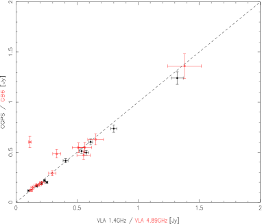
Figure 1: Correlation of VLA 1.4 and 4.89 GHz flux densities with those from the Canadian Galactic Plane Survey at 1.4 GHz and the GB6 catalogue at 4.85 GHz.

These surveys provide data which we believe to be reliable in relation to the fitting procedures used to determine flux densities from the AMI data. We fit power laws to the lower frequency radio data (NVSS 1.4 and VLA 4.89 GHz), the AMI data on its own and the combined data sets. The derived properties of these spectra may be found in Table 5, and are discussed in detail in Section 7.

Since we are using interferometric data we can also fit spectra directly to the visibility measurements in the Fourier plane, a method which is independent of any subjective cleaning procedures. Where we have observed isolated objects the results of these fits agree closely with those found using the data in the map plane, and overall we find there is a good agreement between the two methods. However the complexity of modelling non-isolated extended sources in the uv precludes us from performing all our measurements in this manner.

6.1 Notes on Individual Sources

In the following sections we will discuss the Hii regions in order of Right Ascension.

S175 (Figures 2 and 3). The bipolar nebula S175 is seen at 15.8 GHz to sit in a ring of extended emission, the western side of which is visible in the IRAS 100 $\mu$m data, see Figure 3, and the eastern side of which contains a number of small radio sources visible at 1.4 GHz in the NVSS survey. Also present at radio wavelengths is the Tycho SNR (=G120.1+2.1), still visible at 15.8 GHz approximately one primary beam away from the pointing center. Fitting a modified Planck spectrum of the form $\nu^{2}B(\rm{T})$ (Lagache et al. 2000) to the IRAS 100/60 $\mu$m flux densities we calculate a dust temperature of $T_{\rm{d}}=27.9$ K towards S175. Using the optical recombination line measurements of Hunter (1992) we determine the temperature of the electron gas using the following equation (Haffner, Reynolds & Tufte 1999):

$$\frac{I_{\rm{{\sc{NII}}}}}{I_{\rm{{\sc H\alpha}}}}=1.63\times 10^{5}\left(\frac{N}{{H}}\right)T_{4}^{0.426}\rm{e}^{-2.18/T_{4}},$$ (1)

where $T_{4}$ is the electron gas temperature in units of 10⁴ K. We use the solar ($N$/$H$) = $7.5\times 10^{-5}$ from Meyer, Cardelli, & Sofia (1997) for the gas-phase abundance of N. This gives an electron temperature of $T_{\rm{e}}=7000\pm 200$ K.

The radio spectra of S175 is unusual with a gently climbing spectral index of $\alpha=-0.14$ between 1.4 and 5 GHz. It would be convenient to be able to attribute this rising index to a combination of resolution effects considering the much larger resolution of the GB6 and Effelsberg 100 m dish, and flux losses from the VLA at 1.4 GHz if it were not for the continuation of the index from the low resolution Effelsberg total power flux density at 2.7 GHz to the high resolution VLA interferometric flux density at 4.89 GHz. The good agreement of the GB6 data at 4.85 GHz with the VLA at 4.89 GHz also suggests that there is no flux loss towards this object. A further interesting feature of this spectrum is the apparent bend in the 15 GHz data from the AMI as the data flattens off towards higher frequencies. It is most likely that the rising spectrum between 1.4 and 5 GHz is due to compact knots within the region which are optically thick for $\nu<5$ GHz.

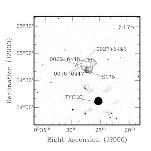
Figure 2: Above: Map of the S175 region. AMI 15.8 GHz contours are overlaid on an NVSS 1.4 GHz greyscale image. Contours increase in powers of 2 from 4 $\sigma$ (i.e. 4,8,16,32,64 etc). Below: Radio spectrum of S175. Data points are integrated flux densities taken from the literature, see Table 6. A best fitting power law is shown as a dashed line.

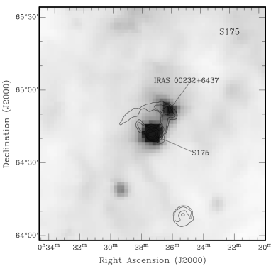
Figure 3: Map of the S 175 region. AMI 15.8 GHz contours are overlaid on an IRAS 100 $\mu$m greyscale image. Contours are as in Figure 2.

S186 (Figure 4) This object is a small nebulosity with a visible 100 $\mu$m IRAS association (IRAS 01056+6251). It is optically thin at low radio frequencies with a flux density of 178 mJy at 330 MHz (Rengelink et al. 1997). From its IRAS 100/60 $\mu$m flux densities we fit a dust temperature of 33.2 K and from optical recombination line data (Hunter 1992) we calculate an electron gas temperature of 7300 K (no uncertainty given). Although the spectral index across the AMI band is slightly steep at $\alpha_{\rm{AMI}}=0.23\pm 1.34$ it is entirely consistent with an overall index of $\alpha^{1.4}_{18}=0.08\pm 0.06$.

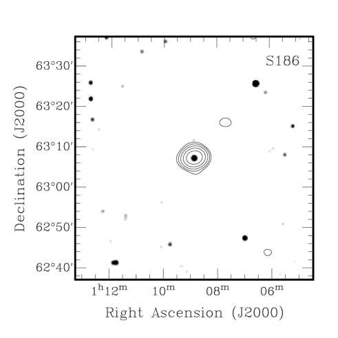
Figure 4: Above: Map of the S186 region. AMI 15.8 GHz contours are overlaid on an NVSS 1.4 GHz greyscale image. Contours are as in Figure 2. Below: Radio spectrum of S186. Data points are integrated flux densities taken from the literature, see Table 6. A best fitting power law is shown as a dashed line.

S211 (Figure 5) This source, otherwise known as LBN 717, is relatively isolated in the radio although at high resolution (Fich 1993) shows a complex structure of small knots embedded in a larger nebulous region. In the radio S211 has been observed at a number of frequencies. We include data at 1.4 GHz from the NVSS and 4.89 GHz from the VLA (Fich 1993); at 2.7 GHz from the Effelsberg 100 m dish (Fürst et al. 1999), which we believe to be useful here due to the relatively isolated nature of this object; data at 4.85 GHz from the GB6 survey, the value of which agrees well with that of the VLA at a different range of angular scales, illustrating the compact nature of this source; and data at 3.2, 6.6 and 10.7 GHz from the Alonquin 46 m dish (Andrew et al. 1973).

The IRAS 100 $\mu$m data show a neighbouring region which we associate with IRAS 04330+5105, however at a distance of 18.5 arcmin it is too far down the primary beam to be detected by AMI. Fitting to the IRAS 100/60$\mu$m flux densities we derive a dust temperature for this region of 31.4 K and from the optical recombination line data of Hunter (1992) we calculate an electron gas temperature of $T_{\rm{e}}=7000\pm 200$ K.

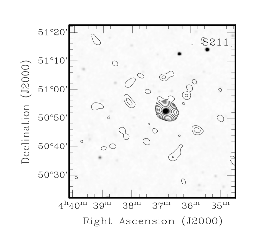
Figure 5: Above: Map of the S211 region. AMI 15.8 GHz contours are overlaid on an NVSS 1.4 GHz greyscale image. Contours are as in Figure 2. Below: Radio spectrum of S211. Data points are integrated flux densities taken from the literature, see Table 6. A best fitting power law is shown as a dashed line.

BFS46 (Figure 6) Also called S235A (Felli et al. 2004; 2006) owing to its close proximity to the more extended S235 Hii region (Sharpless 1959; Felli & Churchwell 1972), BFS46 is a small region of nebulosity. Its spectrum from 1.4 to 5 GHz would suggest partially thick emission due to its rising spectral index (Israel & Felli 1978) but at frequencies above 5 GHz it appears optically thin. The GB6 flux density measurement at 4.85 GHz is unusually low compared to other values at similar frequencies and we suggest that this may be a consequence of difficulty in fitting for a background component in such a densely populated region. We also include data at 4.75, 8.45, 23 and 45 GHz from the VLA (Felli et al. 2006) although we note that the fluxes at 23 and 45 GHz are likely to be affected by flux losses. The spectrum across the AMI band is consistent with optically thin thermal emission, having a spectral index of $\alpha_{\rm{AMI}}=0.12\pm 0.81$. Including VLA data at 1.4 and 4.89 GHz gives an overall spectral index of $\alpha=0.09\pm 0.04$.

Although we obtain a dust temperature of $T_{\rm{d}}=38.5$ K, data do not exist in the literature to calculate an electron gas temperature for this object.

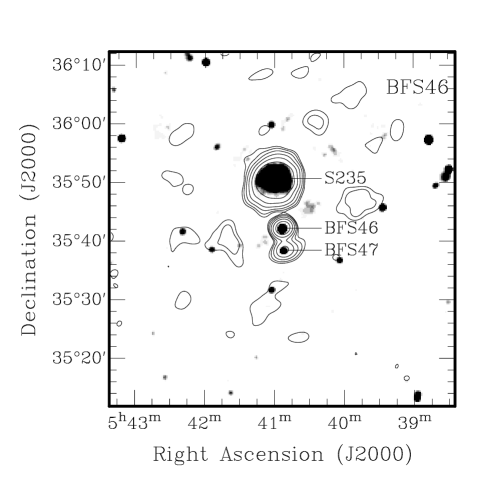
Figure 6: Above: Map of the BFS46 region. AMI 15.8 GHz contours are overlaid on an NVSS 1.4 GHz greyscale image. Contours are as in Figure 2. Below: Radio spectrum of BFS46. Data points are integrated flux densities taken from the literature, see Table 6. In addition data at 4.75, 8.45, 23 and 45 GHz from the VLA are also shown. A best fitting power law is shown as a dashed line.

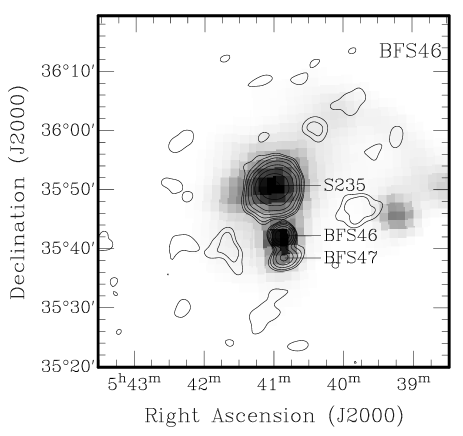
Figure 7: AMI 15.8 GHz contours are overlaid on an IRAS 100 $\mu$m greyscale image. Contours are as in Figure 2.

S259 (Figure 8) The isolated Hii region S259 lies almost directly south of the S254-257 complex. Although it is seen towards the Gemini OB 1 molecular cloud complex it is presumed to be a background source at a distance of 8.3 kpc (Carpenter et al. 1995). In the case of this object the radio emission is far more compact than the IR with a partial ring of IR emission seen to the west (Deharveng et al. 2005) at shorter wavelengths.

At a declination of $\sim 17^{\circ}$ this observation is still heavily affected by satellite interference in the AMI band and the spectral index derived from these frequencies is not well constrained.

Although data are not available in the literature to make an exact calculation of the electron gas temperature of S259 we place an upper limit on the temperature using the H$\alpha$ emission line measurements of Fich, Treffers & Dahl (1990). Assuming that the line width is due largely to Doppler broadening we correct the line widths for the filter response using the simple Gaussian approximation $\Delta\nu_{\rm{D}}=\left[\Delta\nu_{\rm{L}}^{2}-\Delta\nu_{\rm{f}}^{2}\right]^{1/2}$ (Reifenstein et al. 1970). From the corrected line widths we can combine

$$\Delta\nu=\frac{\nu_{0}\Delta V_{\rm FWHM}}{2{c}\sqrt{2{\rm ln}(2)}}$$ (2)

and

$$\Delta\nu=\nu_{0}\sqrt{\frac{{k}T_{\rm e}}{m{c}^{2}}},$$ (3)

to give

$$T_{\rm e}=\frac{m}{k}\left(\frac{\Delta V_{\rm FWHM}}{2\sqrt{2{\rm ln}(2)}}\right)^{2}$$ (4)

(method adapted from Lockman, 1989). In these equations $\Delta\nu$ is the width of the line in frequancy, $\Delta V_{\rm{FWHM}}$ is the width of the line in velocity, $c$ is the speed of light, $k$ is the Boltzmann constant and $m$ is the mass of the atom. For S259 this gives $T_{\rm{e}}\leq 1.3\times 10^{4}$ K. This calculation should provide a generous upper limit as the emission line will also possess a contribution from pressure (collisional) broadening, the magnitude of which will depend on the density of the Hii region.

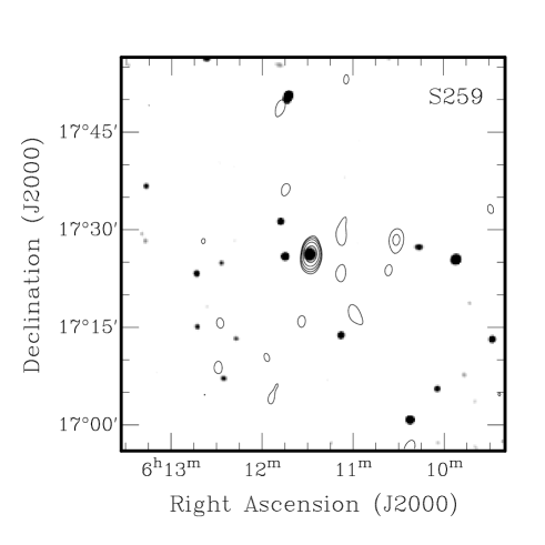
Figure 8: Above: Map of the S259 region. AMI 15.8 GHz contours are overlaid on an NVSS 1.4 GHz greyscale image. Contours are as in Figure 2. Below: Radio spectrum of S259. Data points are integrated flux densities taken from the literature, see Table 6. The best fitting power law is shown as a dashed line.

S256 (Figure 9) The environment of S256 is complex and the object itself is dwarfed by its near neighbours S255 and S257. These sources were excluded from the sample due to their large angular extent and consequent flux losses for AMI. However, their proximity means that at the resolution of the AMI our single channel signal-to-noise is not good enough in this instance to produce separate maps. Therefore we present only a combined map and flux density for this object.

We estimate an upper limit on the electron gas temperature of S256 using Equation 4 to find $T_{\rm{e}}\leq$ 22 300 K. The line width of S256 is broad at 32.3 km s^-1 (corrected) indicating that this is a dense Hii region.

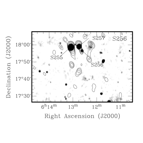
Figure 9: Above: Map of the S256 region. AMI 15.8 GHz contours are overlaid on an NVSS 1.4 GHz greyscale image. Contours are as in Figure 2. Below: Radio spectrum of S256. Data points are integrated flux densities taken from the literature, see Table 6. The best fitting power law is shown as a dashed line.

S271 (Figure 10) The true nature of S271 is a matter of debate. Although it was originally thought to be an Hii region there is considerable evidence that it may be in fact a planetary nebula (PN). This is supported by the IRAS flux densities which show a spike at 60 $\mu$m with an excess of $>100$ Jy relative to the 12, 25 and 100 $\mu$m bands. Consequently we cannot fit a dust temperature for this object but do calculate an electron gas temperature of $T_{\rm{e}}=7200\pm 500$ K from recombination line data (Hunter 1992).

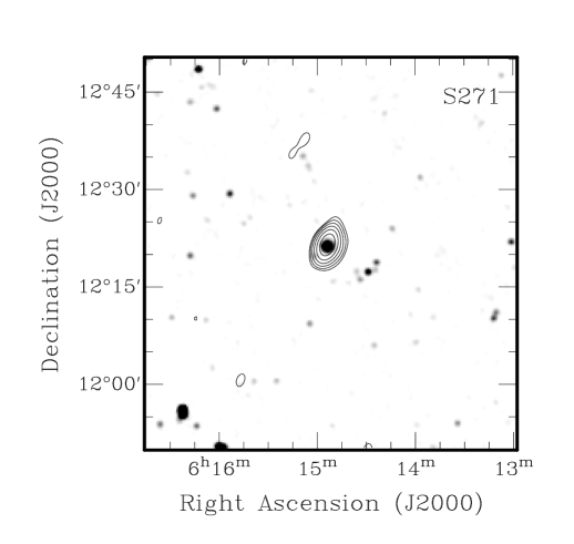
Figure 10: Above: Map of the S271 region. AMI 15.8 GHz contours are overlaid on an NVSS 1.4 GHz greyscale image. Contours are as in Figure 2. Below: Radio spectrum of S271. Data points are integrated flux densities taken from the literature, see Table 6. The best fitting power law is shown as a dashed line.

In the AMI band this source is heavily contaminated by satellite interference and although we measure a reasonable spectrum for channels 3 to 5 we then see a turn over in the data. In the absence of any physical mechanism for this turn over we must conclude that it arises as a consequence of poor calibration due to satellite interference. Simulations using the visibility data show that there should be no significant ($>$ 1%) flux loss over the AMI band and, although the phase errors are quite large due to the contaminating signal, self-calibrating the data has little effect.

S288 (Figure 11) This source has a declination of $-4$ degrees, right on the limit of AMI’s field of view. At this declination interference from geostationary satellites contaminates the data severely and consequently the errors on our data are significantly larger than in the case of higher declination sources. This is a pity since S288 is a small bright nebula, comparatively isolated and with a luminous association seen at 100 $\mu$m in the IRAS data. In spite of this contamination we still measure a reasonable microwave spectrum with a spectral index of $\alpha=0.18\pm 0.06$ across the AMI band. However, we urge caution due to the poor nature of the data. From the IRAS 100/60 $\mu$m flux densities we fit a dust temperature of $T_{\rm{d}}=35.4$ K and from recombination line ratios we calculate a gas temperature of $T_{\rm{e}}=6600\pm 400$ K.

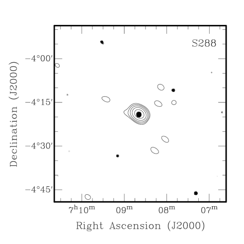
Figure 11: Above: Map of the S288 region. AMI 15.8 GHz contours are overlaid on an NVSS 1.4 GHz greyscale image. Contours are as in Figure 2. Below: Radio spectrum of S288. Data points are integrated flux densities taken from the literature, see Table 6. The best fitting power law is shown as a dashed line.

S100 (Figure 12) The S100/99 complex is poorly resolved by the PSF of the AMI. We measure a peak flux density towards this complex of $S_{\rm{p}}=8.28\pm 0.41$ Jy bm^-1. Although we present our combined channel map here we have not compiled spectra for the different sources since the complicated nature of the region makes higher resolution necessary for extracting reliable flux densities.

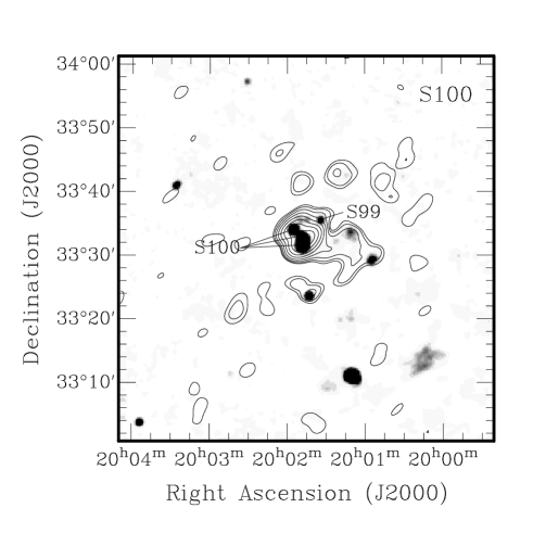
Figure 12: Map of the S 99/100 region. AMI 15.8 GHz contours are overlaid on an NVSS 1.4 GHz greyscale image. Contours are as in Figure 2.

S121 (Figure 13) This source is the most extended in our sample and is poorly fitted by a Gaussian at higher frequencies. Channels 6 and 7 of the AMI data show severe ($>$ 20%) flux loss towards this object due to a lack of short spacings caused by necessary flags in the data. Using the visibility coverage of these channels and the total power maps of the CGPS we are able to calculate these losses and their corrected flux densities are indicated in Figure 13 by an arrow. The IRAS 100 $\mu$m emission closely traces the 15.8 GHz map with extensions to the north and south-east. Fitting a modified Planck spectrum to the IRAS 100/60 $\mu$m flux densities gives a dust temperature of $T_{\rm{d}}=28.8$ K. Vallee (1983) derived the electron gas temperature of this region, $T_{\rm{e}}=9000$ K, from observations of the H85$\alpha$ radio recombination line and measured the emission measure to be $8\times 10^{4}$ pc cm^-6. The spectrum of S121 is shown in Figure 13; in addition to VLA data points at 1.4 and 4.89 GHz (Fich 1993) we include data at 10.5 GHz taken by Vallee (1983) with the Alonquin 46 m dish.

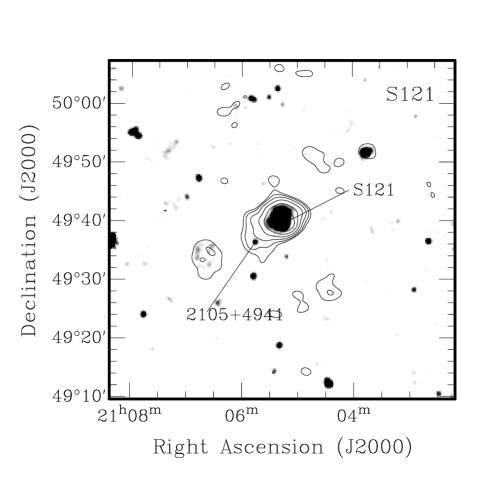
Figure 13: Above: Map of the S121 region. AMI 15.8 GHz contours are overlaid on an NVSS 1.4 GHz greyscale image. Contours are as in Figure 2. Below: Radio spectrum of S121. Data points are integrated flux densities taken from the literature, see Table 6. Arrows indicate the calculated correction for flux losses. The best fitting power law is shown as a dashed line.

Table 4: Dust and gas temperatures for the AMI Hii region sample.

Name	$T_{\rm{dust}}$	$T_{\rm{e}}$
	(K)	(K)
S175	27.9	$7000\pm 200$
S186	33.2	7300
S211	19.2	$7000\pm 200$
BFS46	38.5	-
S259	29.2	$\leq$13000
S256	18.7	$\leq$22300
S271	-	$7200\pm 500$
S288	35.4	$6600\pm 400$
S121	28.8	9000(1)
S127	30.3	$10500\pm 820$
BFS10	29.0	-
S138	35.4	6300(2), 11200(3)
S149	31.4	$7500\pm 400$, $8600\pm 495^{(4)}$
S152	30.4	8400(5), $9100\pm 900^{(6)}$
S167	33.3	$\leq$7625

Notes:–Temperatures are calculated as described in the text with the exceptions of (1) Vallee (1983), (2) Deharveng et al.(1999), (3),(5) Afflerbach (1997), (4) Matthews (1981), and (6) Wink (1983).

S127 (Figure 14) Otherwise known as LBN 436 this region in fact contains two compact Hii regions (WB 85A and WB 85B) which are unresolved by the AMI. Indeed at such small separation the flux density of S127 as found in the literature frequently comprises both objects. In Figure 14 we show data from NVSS at 1.4 GHz; 2.7 GHz data from Paladini et al. (2003) re-analysed from the Effelsberg 100 m telescope; 4.89 GHz data (Fich 1993) and 4.86 GHz (Rudolph et al. 1996) from the VLA. We also include data at 8.44 GHz and 15 GHz (Rudolph et al. 1996) from the VLA, although we do not use these data for fitting purposes as we believe them to be heavily affected by flux losses. We allow the poorer resolution Effelsberg data in this instance due to the relatively isolated nature of the complex.

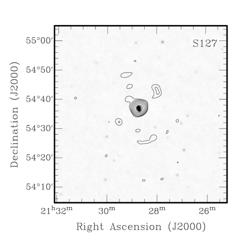
Figure 14: Above: Map of the S127 region. AMI 15.8 GHz contours are overlaid on an NVSS 1.4 GHz greyscale image. Contours are as in Figure 2. Below: Radio spectrum of S127. Data points are integrated flux densities taken from the literature, see Table 6. In addition data at 4.86, 8.44 and 15 GHz from the VLA are also shown. The best fitting power law is shown as a dashed line.

The IRAS 100 $\mu$m emission is very similar to that at 15.8 GHz, with no secondary sources in the field. Fitting a modified Planck spectrum to the 100 and 60 $\mu$m data gives a dust temperature of 30.3 K. Significant excess is present at shorter IR wavelengths indicating the presence of a second hotter dust component. Although radio recombination line or optical recombination line data are not available for this object we can estimate the temperature of the electron gas using its distance from the Galactic centre (Afflerbach, Churchwell & Werner 1997).

$$T_{{\rm e}}/{\rm K}=(4560\pm 220)+(390\pm 40)(D_{{\rm G}}/{\rm kpc}).$$ (5)

We note that at a distance of $D_{\rm{G}}$=15 kpc from the Galactic center S127 is outside the range of data fitted to derive this relation. However, the calculated temperature of 10500$\pm 820$ K is similar to that extrapolated from measurements by Fich & Silkey (1991) which suggest a value of 10⁴ K in the far outer galaxy.

BFS10 (Figure 15) The CO selected Hii region BFS10 is a little studied object. It is dwarfed on larger scales by the neighbouring Hii complexes S131 and DA568. We fit a dust temperature of $T_{\rm{d}}=29.0$ K. We see an increased amount of flux in AMI channel 3 towards BFS10. This seems to be caused by an amount of extended emission associated with this object which is seen on the largest scales only. This extended emission may also be the cause of the slight discrepancy between the VLA and GB6 fluxes at 4.8 GHz. It does not appear to be immediately obvious in the map plane but is visible as structure on large angular scales in the visibility data of channel 3; the visibility coverage of which extends to slightly larger angular scales then channels 4–8 due to its lower frequency.

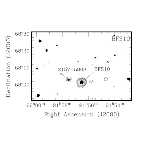
Figure 15: Above: Map of the BFS10 region. AMI 15.8 GHz contours are overlaid on an NVSS 1.4 GHz greyscale image. Contours are as in Figure 2. Below: Radio spectrum of BFS10. Data points are integrated flux densities taken from the literature, see Table 6. The best fitting power law is shown as a dashed line.

S138 (Figure 16) This Hii region, associated with IRAS 22308+5812, is in a complex region at both radio and infra-red wavelengths. In the radio the flux density measurement of the GB6 survey at 4.85 GHz is confused by the nearby source NVSS 2232+5832. The 100$\mu$m IRAS data shows a broad band of diffuse emission around S138 and a neighbouring source to the south-west. The radio continuum data at 15.8 GHz also shows an extension to the south-west consistent with the position of both the radio and IR source (IRAS 22306+5809). From the Nii and H$\alpha$ spectral measurements of Deharveng et al. (1999) we can derive an electron gas temperature for the region, using Equation 1. The value of $T_{\rm{e}}=6300$ K that we calculate is somewhat lower than that of Afflerbach et al. (1997) who derive a temperature of 11200 K using the ratio of infra-red fine structure lines to the radio continuum at lower frequencies. We suggest that this may be a consequence of the optical recombination line measurements being taken in the direction of the main exciting star where the electron density is highest (N${}_{\rm{e}}\simeq 1000$ cm^-3), compared to the outer regions of the nebula where it falls to $\sim$200 cm^-3 (Deharveng 1999), which is more in line with the value calculated by Afflerbach of 175 cm^-3. From the IRAS 100/60 $\mu$m flux densities we calculate a dust temperature, $T_{\rm{d}}=35.4$ K.

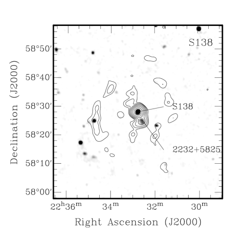
Figure 16: Above: Map of the S138 region. AMI 15.8 GHz contours are overlaid on an NVSS 1.4 GHz greyscale image. Contours are as in Figure 2. Below: Radio spectrum of S138. Data points are integrated flux densities taken from the literature, see Table 6. The best fitting power law is shown as a dashed line.

S149 (Figure 17) The source we identify with S149 is in reality both S149 and S148, whose small separation makes them indistinguishable at the resolution of AMI. The S147 Hii region is also visible as an extension to the south-west of the main source. All three sources are visible in the IRAS 100 $\mu$m data as is a diffuse extension to the north of the main source, which possesses no radio counterpart. Fitting to the IRAS 100/60 $\mu$m flux densities we find a dust temperature of $T_{\rm{d}}=31.4$ K for S149; and using Equation 1 and the optical recombination line data of Hunter et al. (1992) we find an electron gas temperature of $T_{\rm{e}}=7500\pm 400$ K, slightly lower than that of Matthews (1981) who found $T_{\rm{e}}=8600\pm 495$ K.

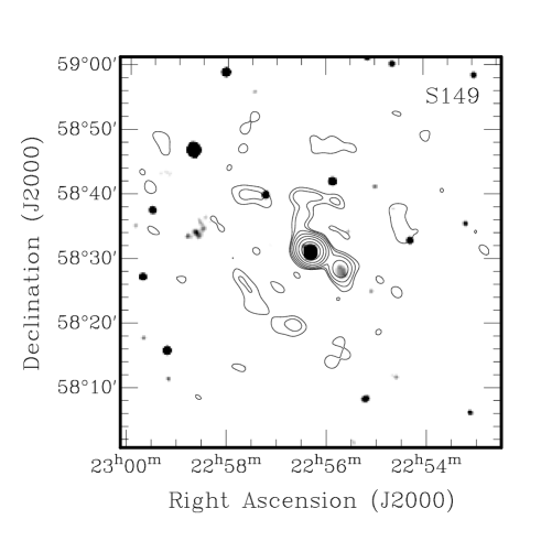
Figure 17: Above: Map of the S149 region. AMI 15.8 GHz contours are overlaid on an NVSS 1.4 GHz greyscale image. Contours are as in Figure 2. Below: Radio spectrum of S149. Data points are integrated flux densities taken from the literature, see Table 6. The best fitting power law is shown as a dashed line.

S152 (Figure 18) The radio emission from S152 appears slightly offset from the IRAS 100 $\mu$m peak. There is a large diffuse patch of radio emission to the south-east of the object, see Figure 18, which has no corresponding IR counterpart although there are several IR sources nearby. The electron gas temperature calculated by Afflerbach et al. (1997) of $T_{\rm{e}}=8400$ K agrees well with that of Wink et al. (1983) who find $T_{\rm{e}}=9100\pm 900$ K using the RRL H76$\alpha$.

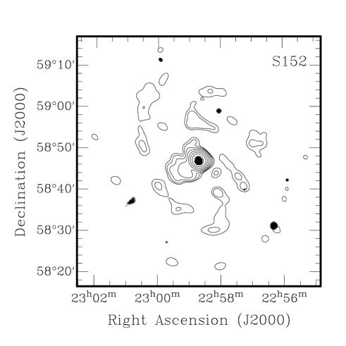
Figure 18: Above: Map of the S152 region. AMI 15.8 GHz contours are overlaid on an NVSS 1.4 GHz greyscale image. Contours are as in Figure 2. Below: Radio spectrum of S152. Data points are integrated flux densities taken from the literature, see Table 6. In addition data at 8.35 GHz from the Galactic plane survey of Langston (2000) are also shown. The best fitting power law is shown as a dashed line.

S167 (Figure 19) Although originally classified as a planetary nebula further investigation confirmed the status of S167 as an Hii region (Acker 1990). At 15.8 GHz we see a relatively compact source with slight extensions to the north and south-east, the first of these coinciding with the radio source NVSS 2335+6455. We observe a relatively constant spectral index from 1.4 to 18 GHz with $\alpha_{\rm{AMI}}=0.16\pm 0.54$ and an overall index of $\alpha_{18}^{1.4}=0.13\pm 0.06$.

As with S256 and S259 we can only place an upper limit on the electron gas temperature of S167 and find, using Equation 4, $T_{\rm{e}}\leq$ 7625 K.

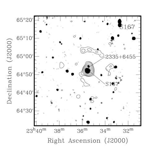
Figure 19: Above: Map of the S167 region. AMI 15.8 GHz contours are overlaid on an NVSS 1.4 GHz greyscale image. Contours are as in Figure 2. Below: Radio spectrum of S167. Data points are integrated flux densities taken from the literature, see Table 6. The best fitting power law is shown as a dashed line.

Table 5: AMI Hii sample

Name	S${}^{15}_{\rm{i}}$	$\alpha_{1.4}^{4.9}$	$\alpha_{\rm{AMI}}$	$\alpha_{\rm{tot}}$	Sexcess	Excess 100$\mu$m emissivity
	(Jy)				(mJy)	$\mu$K(MJy/sr)-1
	[2]	[3]	[4]	[5]	[6]	[7]
S175	$0.095\pm 0.005$	-0.15$\pm$0.36	0.51$\pm$2.82	0.04$\pm$0.07	$<83$	$<60$
		0.10			$<11$	$<6$
S186	$0.144\pm 0.007$	0.02$\pm$0.09	0.27$\pm$1.34	0.07$\pm$0.06	$<21$	$<11$
		0.10			$<29$	$<15$
S211	$0.568\pm 0.028$	0.20$\pm$0.07	0.06$\pm$0.05	0.14$\pm$0.02	25${}^{+47}_{-45}$	$13$
		0.10			$<114$	$<60$
BFS46	$0.201\pm 0.010$	0.02$\pm$0.06	0.12$\pm$0.81	0.09$\pm$0.04	$<1$	$<1$
		0.10			$<28$	$<6$
S259a…	$0.071\pm 0.004$	-0.03$\pm$0.13	0.48$\pm$5.66	0.29$\pm$0.29	-	-
		0.10			$<1$	$<1$
S256a…	$0.094\pm 0.010$	0.26$\pm$0.55	-	0.21$\pm$0.31	9${}^{+75}_{-41}$	3
		0.10			$<21$	$<6$
S271a,b…	$0.185\pm 0.020$	0.08$\pm$0.11	1.01$\pm$5.67	0.27$\pm$0.23	$<1$	$<1$
		0.10			$<1$	$<1$
S288a…	$0.440\pm 0.044$	0.06$\pm$0.04	0.25$\pm$1.41	0.18$\pm$0.06	$<1$	$<1$
		0.10			$<46$	$<23$
S121	$0.440\pm 0.022$	0.02$\pm$0.05	-0.08$\pm$0.26	0.07$\pm$0.01	$1^{+37}_{-35}$	$<1$
		0.10			$7^{+44}_{-44}$	8
S127	$0.415\pm 0.021$	0.07$\pm$0.05	0.19$\pm$0.41	0.16$\pm$0.02	$<1$	$<1$
		0.10			$<20$	$<19$
BFS10	$0.135\pm 0.007$	0.08$\pm$0.16	0.38$\pm$2.05	0.19$\pm$0.09	$<32$	$<39$
		0.10			$<2$	$<2$
S138	$0.394\pm 0.020$	-0.03$\pm$0.03	0.25$\pm$0.51	0.13$\pm$0.03	-	-
		0.10			$<6$	$<2$
S149	$0.410\pm 0.021$	0.09$\pm$0.07	0.25$\pm$0.39	0.14$\pm$0.01	$<29$	$<20$
		0.10			$<53$	$<34$
S152	$1.048\pm 0.052$	-0.04$\pm$0.06	0.17$\pm$0.10	0.11$\pm$0.01	-	-
		0.10			$<81$	$<16$
S167	$0.175\pm 0.009$	0.08$\pm$0.14	0.16$\pm$0.54	0.13$\pm$0.06	$<48$	$<42$
		0.10			$<23$	$<23$

Notes:– [2] 15.8 GHz integrated flux densities, [3] spectral index calculated from 1.4 and 4.89 GHz VLA data; [4] spectral index fitted to the 6 spectral channels of the AMI, [5] overall spectral index including both VLA and AMI data; [6] derived excess emission at 15.8 GHz, upper limits are at $2\sigma$, $\sim$95%; [7] excess 100 $\mu$m emissivity following the method of Dickinson et al. (2007). (a) Significant satellite interference; (b) Planetary Nebula

7 Discussion

Hii regions are a reasonable place to look for anomalous emission since their general radio behaviour is well understood. In the region of the spectrum above approximately 1 GHz they are dominated by thermal free-free emission with a canonical spectral index of $\alpha=0.1$. In an idealized sense this emission arises from a sphere of ionized gas surrounding a hot star, or cluster of stars; although the Hii region itself may consist of several compact objects which are unresolved by the synthesized beam of the AMI. In addition to this, Hii regions are strong emitters in the IR making them suitable candidates for spinning dust emission, and have dust temperatures typically in the range 30–50 K. All the objects presented here have temperatures consistent with this range, see Table 4, with the exception of S211 which has a slightly lower dust temperature. These objects are not necessarily perfect blackbodies and detailed modelling of the dust properties, the geometry and the possible spectral features in the IRAS bands is beyond the scope of this paper. For more detailed analysis of the infrared content of Hii regions see, for example, Akabane & Kuno (2005).

The spectrum of optically thin thermal emission varies slowly with frequency and electron gas temperature, but in the frequency range used here it can be described well by a single index of $\alpha=0.1$. Indeed from our sample of Hii regions we find an average spectral index between 1.4 and 5 GHz of $\alpha=0.05\pm 0.09$, which is consistent with this value. Where possible we have calculated the electron gas temperature of each Hii region from data available in the literature. We find that for all those sources where data are available the electron gas temperature of falls within the expected range (see Table. 4). Furthermore we also find that the flux densities measured at 15.8 GHz by the AMI are also consistent with this index.

Within the AMI band the average spectral index tends to be steeper, $\alpha=0.29\pm 0.25$, but is not significantly different from the canonical index of $\alpha=0.1$. Overall we find an average spectral index of $\alpha^{17.6}_{1.4}=0.15\pm 0.07$. This confirms the dominance of free–free emission in these bright Hii regions.

The aim of this study was to investigate a possible excess of emission within the AMI band which might be attributed to a spinning dust component. The AMI is particularly suitable for this type of measurement since the spinning dust predictions of Drain & Lazarian (1998a,b) imply that the peak of the resulting spectrum will lie close to 15 GHz. In spite of this we see no evidence for an excess in the sources we observe here. In Table 5 we present the combined channel flux density of each source at 15.8 GHz, the spectral index from the VLA radio measurements at 1.4 and 4.89 GHz, the spectral index calculated using only the data from the six AMI channels, and the spectral index found using both VLA and AMI data. We note that the uncertainties on the spectral indices calculated using AMI data alone include errors which are correlated between the channels, and that this leads to an overestimation of the uncertainty in each spectral index. The average difference between the spectral index calculated within the AMI band and the overall index from 1.4 to 17.9 GHz is 0.19 and this is perhaps a better representation of the non-systematic error in this quantity. In addition to these derived quantities we also calculate the excess towards each Hii region at 15.8 GHz. We do this in two ways: firstly by extrapolating the spectral index calculated from the VLA data, $\alpha_{1.4}^{4.9}$; secondly using the canonical spectral index of $\alpha=0.1$. Column 6 of Table 5 shows the calculated excess at 15.8 GHz relative to these two indices. In the case that a positive excess is not found and instead there is a decrement at 15.8 GHz towards an object then the 2 $\sigma$ upper limit is shown. In the case that the 2 $\sigma$ upper limit is still a decrement with respect to the flux density predicted from the spectral index then the excess is marked $<1$. From Table 5 it can be seen that a positive difference in flux density with respect to that predicted from the extrapolated spectral index is seen only in four of the fifteen Hii regions tabulated here; but that in each of these instances the excess is not significant at even the 1 $\sigma$ level.

Combining the predictions we see that the average excess towards this sample of fifteen Hii regions is $-75$ mJy extrapolating the derived spectral index. Using a canonical index of $\alpha=0.1$ we see an average excess of $-49$ mJy. These results would suggest that, not only is there no evidence for anomalous emission in the spectra of these objects, but also that there is a slight steepening of the spectral index as we move to higher frequencies (Dickinson et al. 2003).

This result differs to that of Dickinson et al. (2007) who found a slight excess of emission at 31 GHz for a sample of southern Hii regions. In terms of the physical characteristics (dust/electron temperature) the two samples are similar. Observationally the measurements of Dickinson et al. were made for a range of slightly larger angular scales, and although we have shown flux losses not to be significant, this only relates to the free–free emission and not to any possible anomalous component. It has been suggested that the anomalous emission is distributed more diffusely (de Olivera–Costa et al. 2002), and is consequently affected to a larger degree. However, given the compact nature of these objects this seems unlikely.

All the objects observed here have bright dust associations and we investigated the correlation of the 15.8 GHz flux with that found in each of the 12, 25, 60 and 100 $\mu$m bands of IRAS. After omitting two outlying objects, namely BFS46 and S256, the fluxes of which are artificially high in the IRAS data due to resolution effects, we performed a Pearson correlation analysis. We find a positive correlation for all four IRAS bands with the strongest correlation occuring in the 100 $\mu$m band ($r$ = 0.88). The correlation between the AMI 15.8 GHz flux densities and those of the VLA at 1.4 GHz is much stronger ($r$ = 0.99), suggesting that the emission we see at 15.8 GHz is indeed simply free–free rather than dust emission. We note, however, that dust emission will depend heavily on the dust conditions (i.e. temperature, density) within the cloud, and any variance in these conditions would reduce the degree of correlation.

The limits on any excess have been converted to a dust emissivity relative to the IRAS 100 $\mu$m map, see Column 7 of Table 5. This conversion is model independent (Dickinson et al. 2003) and although we have used IRAS here other authors have also calculated dust emissivites relative to different standards such as the DIRBE 140 $\mu$m map, the Schlegel, Finkbeiner & Davis (1998) 100$\mu$m map, or the Finkbeiner, Davis & Schlegel (1999) model 8 map normalized at 94 GHz. Our three positive differences in flux density: S211, S121 and S256, are all consistent with the expected emissivity value of $\sim 10\mu\rm{K}(\rm{MJy/sr})^{-1}$ at high latitudes (Davies et al. 2006).

8 Conclusions

The observations of fifteen bright Hii regions and one planetary nebula reported here show no evidence for anomalous emission due to spinning dust at six frequencies between 14 and 18 GHz. This result confirms the dominance of free-free emission in these objects with a spectral index consistent with the canonical value of 0.1. No significant evidence for spinning dust emission has been found.

9 ACKNOWLEDGEMENTS

We thank the staff of the Lord’s Bridge observatory for their invaluable assistance in the commissioning and operation of the Arcminute Microkelvin Imager. The AMI is supported by the STFC. NHW and MLD acknowledge the support of a PPARC studentship. We also thank the anonymous referee for their useful comments.

Table 6: Radio flux densities.

	Freq. (GHz)
	1.4(1)	2.7(2)	3.2(3)	4.85(4)	4.89(5)	6.6(3)	8.45	10.7(3)
Name	(Jy)	(Jy)	(Jy)	(Jy)	(Jy)	(Jy)	(Jy)	(Jy)
S175…	0.102$\pm$0.004	0.11	0.120$\pm$0.011	-	0.120	0.123$\pm$0.012	-	-
S186…	0.169$\pm$0.007	0.18	-	0.169$\pm$0.015	0.165	-	-	-
S211…	0.800$\pm$0.025	0.74	0.75$\pm 0.10$	0.627$\pm 0.056$	0.652	0.6$\pm$0.01	-	0.6$\pm$0.01
BFS46..	0.253$\pm$0.008	-	-	0.213$\pm$0.021	0.248	-	0.248$\pm$0.012(7)	-
S259…	0.132$\pm$0.005	-	-	0.146$\pm$0.015	0.136	-	-	-
S256…	0.158$\pm$0.016	-	-	-	0.114	-	-	-
S271…	0.330$\pm$0.011	0.32	-	0.290$\pm$0.026	0.297	-	-	-
S288…	0.638$\pm$0.024	0.68	0.90$\pm$0.15	-	0.595	0.6$\pm$0.1	-	0.5$\pm$0.1
S121…	0.539$\pm$0.011	-	-	0.484$\pm$0.043	-	-	-	-
S127…	0.602$\pm$0.010	0.6$\pm$0.2(8)	-	0.577$\pm 0.058$	0.563	-	0.267$\pm$0.026(6)	-
BFS10..	0.210$\pm$0.007	-	-	0.176$\pm$0.016	0.190	-	-	-
S138…	0.537$\pm$0.019	-	-	0.470$\pm$0.042	0.554	-	-	-
S149…	0.575$\pm$0.019	-	-	0.545$\pm$0.048	0.512	-	-	-
S152…	1.320$\pm$0.050	1.56	-	1.360$\pm$0.140	1.380	-	-	-
S167…	0.233$\pm$0.008	-	-	0.196$\pm$0.017	0.212	-	-	-

Notes:– Radio flux densities from the literature. Where no error is quoted an uncertainty of 10 per cent has been assumed.
References:– (1) Condon et al. (1998), (2) Fürst et al. (1990), (3) Andrew et al. (1973), (4) Gregory (1996), (5) Fich (1993), (6) 8.44 GHz Rudolph et al. (1996), (7) 8.45 GHz Felli et al (2006), (8) Paladini et al. 2003)

Table 7: AMI flux densities.

	Freq. (GHz)
	14.2	15.0	15.7	16.4	17.1	17.9
Name	(Jy)	(Jy)	(Jy)	(Jy)	(Jy)	(Jy)
S175…	0.103$\pm$0.005	0.098$\pm$0.005	0.095$\pm$0.005	0.092$\pm$0.005	0.092$\pm$0.005	0.091$\pm$0.005
S186…	0.147$\pm$0.008	0.146$\pm$0.007	0.144$\pm$0.007	0.140$\pm$0.007	0.139$\pm$0.007	0.139$\pm$0.007
S211…	0.567$\pm$0.025	0.559$\pm$0.025	0.568$\pm$0.025	0.571$\pm$0.025	0.559$\pm$0.025	0.566$\pm$0.025
BFS46..	0.209$\pm$0.010	0.206$\pm$0.010	0.201$\pm$0.010	0.209$\pm$0.010	0.205$\pm$0.010	0.200$\pm$0.010
S259…	0.075$\pm$0.005	0.068$\pm$0.005	0.071$\pm$0.005	0.065$\pm$0.005	0.068$\pm$0.005	0.065$\pm$0.005
S256…	-	-	0.094$\pm$0.010	-	-	-
S271…	0.195$\pm$0.020	0.185$\pm$0.020	0.185$\pm$0.020	0.176$\pm$0.020	0.163$\pm$0.020	0.151$\pm$0.020
S288…	0.434$\pm$0.043	0.412$\pm$0.041	0.440$\pm$0.044	0.420$\pm$0.042	0.456$\pm$0.046	0.385$\pm$0.039
S121…	0.453$\pm$0.026	0.435$\pm$0.026	0.440$\pm$0.025	0.461$\pm$0.023	0.380$\pm$0.022	0.332$\pm$0.020
S127…	0.427$\pm$0.021	0.422$\pm$0.021	0.415$\pm$0.021	0.411$\pm$0.021	0.405$\pm$0.020	0.408$\pm$0.020
BFS10..	0.149$\pm$0.007	0.138$\pm$0.007	0.135$\pm$0.007	0.133$\pm$0.006	0.132$\pm$0.006	0.128$\pm$0.006
S138…	0.411$\pm$0.020	0.406$\pm$0.020	0.394$\pm$0.020	0.402$\pm$0.020	0.387$\pm$0.020	0.387$\pm$0.020
S149…	0.424$\pm$0.020	0.418$\pm$0.020	0.410$\pm$0.020	0.408$\pm$0.020	0.392$\pm$0.020	0.407$\pm$0.020
S152…	1.065$\pm$0.050	1.057$\pm$0.050	1.048$\pm$0.050	1.041$\pm$0.050	1.033$\pm$0.050	1.026$\pm$0.050
S167…	0.164$\pm$0.008	0.165$\pm$0.008	0.164$\pm$0.008	0.165$\pm$0.008	0.149$\pm$0.007	0.154$\pm$0.008

Notes:– Flux densities measured by the AMI telescope. No correction has been made for flux losses. See text for details.

References

- Akabane & Kuno (2005) Akabane K., Kuno N., 2005, A&A, 431, 183
- Acker & Stenholm (1990) Acker A., Stenholm B., 1990, A&AS, 86, 219
- Afflerbach, Churchwell, & Werner (1997) Afflerbach A., Churchwell E., Werner M. W., 1997, ApJ, 478, 190
- Andrew et al. (1973) Andrew B. H., Ehman J. R., Gearhart M. R., Kraus J. D., 1973, ApJ, 185, 137
- Baars et al. (1977) Baars J. W. M., Genzel R., Pauliny-Toth I. I. K., Witzel A., 1977, A&A, 61, 99
- Becker, White, & Edwards (1991) Becker R. H., White R. L., Edwards A. L., 1991, ApJS, 75, 1
- Blitz et al. (1982) Blitz, L., Fich, M., & Stark, A. A. 1982, ApJS, 49, 183
- Browne et al. (1998) Browne, I. W. A., Wilkinson, P. N., Patnaik, A. R., & Wrobel, J. M. 1998, MNRAS, 293, 257
- Carpenter, Snell, & Schloerb (1995) Carpenter J. M., Snell R. L., Schloerb F. P., 1995, ApJ, 445, 246
- Casassus, Readhead, Pearson, Nyman, Shepherd Bronfman (2004) Casassus S., Readhead A. C. S., Pearson T. J., Nyman L. -L., Shepherd M. C., Bronfman L., 2004, ApJ, 603, 599
- Casassus et al. (2006) Casassus S., Cabrera G. F., Förster F., Pearson T. J., Readhead A. C. S., Dickinson C., 2006, ApJ, 639, 951
- Condon et al. (1998) Condon J. J., Cotton W. D., Greisen E. W., Yin Q. F., Perley R. A., Taylor G. B., Broderick J. J., 1998, AJ, 115, 1693
- Davies et al. (2006) Davies R. D., Dickinson C., Banday A. J., Jaffe T. R., Górski K. M., Davis R. J., 2006, MNRAS, 370, 1125
- Day, Caswell, & Cooke (1972) Day G. A., Caswell J. L., Cooke D. J., 1972, AuJPA, 25, 1
- Deharveng et al. (1999) Deharveng L., Zavagno A., Nadeau D., Caplan J., Petit M., 1999, A&A, 344, 943
- Deharveng, Zavagno, & Caplan (2005) Deharveng L., Zavagno A., Caplan J., 2005, A&A, 433, 565
- de Oliviera-Costa et al. (2002) de Oliviera-Costa A., et al., 2002, ApJ, 567, 363
- de Oliviera-Costa et al. (2004) de Oliviera-Costa A., Tegmark M., Davies R. D., Gutiérrez C. M., Lasenby A. N., Rebolo R., Watson R. A., 2004, ApJ, 606, L89
- Dickinson et al. (2007) Dickinson C., Davies R. D., Bronfman L., Casassus S., Davis R. J., Pearson T. J., Readhead A. C. S., Wilkinson P. N., 2007, MNRAS, 379, 297
- Dickinson et al. (2006) Dickinson C., Casassus S., Pineda J. L., Pearson T. J., Readhead A. C. S., Davies R. D., 2006, ApJ, 643, L111
- Dickinson, Davies, & Davis (2003) Dickinson C., Davies R. D., Davis R. J., 2003, MNRAS, 341, 369
- Draine & Lazarian (1998a) Draine B. T., Lazarian A., 1998a, ApJ, 494, L19
- Draine & Lazarian (1998a) Draine B. T., Lazarian A., 1998b, ApJ, 508, 157
- Draine & Lazarian (1999) Draine B. T., Lazarian A., 1999, ApJ, 512, 740
- Felli & Churchwell (1972) Felli M., Churchwell E., 1972, A&AS, 5, 369
- Felli et al. (1978) Felli M., Harten R. H., Habing H. J., Israel F. P., 1978, A&AS, 32, 423
- Felli et al. (2004) Felli M., Massi F., Navarrini A., Neri R., Cesaroni R., Jenness T., 2004, A&A, 420, 553
- Felli et al. (2006) Felli M., Massi F., Robberto M., Cesaroni R., 2006, A&A, 453, 911
- Fich (1993) Fich M., 1993, ApJS, 86, 475
- Fich & Silkey (1991) Fich M., Silkey M., 1991, ApJ, 366, 107
- Fich, Dahl, & Treffers (1990) Fich M., Dahl G. P., Treffers R. R., 1990, AJ, 99, 622
- Finkbeiner (2004) Finkbeiner D. P., 2004, ApJ, 614, 186
- Finkbeiner, Davis, & Schlegel (1999) Finkbeiner D. P., Davis M., Schlegel D. J., 1999, ApJ, 524, 867
- Finkbeiner et al. (2002) Finkbeiner D. P., Schlegel D. J., Frank C., Heiles C., 2002, ApJ, 566, 898
- Finkbeiner et al. (2004) Finkbeiner D. P., Langston G. I., Minter A. H., 2004, ApJ, 617, 350
- Frst et al. (1990) Frst E., Reich W., Reich P., Reif K., 1990a, A&AS, 85, 691
- Frst et al. (1990) Frst E., Reich W., Reich P., Reif K., 1990b, A&AS, 85, 805
- Gregory & Taylor (1986) Gregory P. C., Taylor A. R., 1986, AJ, 92, 371
- Gregory et al. (1996) Gregory, P. C., Scott, W. K., Douglas, K., & Condon, J. J. 1996, ApJS, 103, 427
- Haffner, Reynolds, & Tufte (1999) Haffner L. M., Reynolds R. J., Tufte S. L., 1999, ApJ, 523, 223
- Hunter (1992) Hunter D. A., 1992, ApJS, 79, 469
- Israel (1976) Israel F. P., 1976a, A&A, 48, 193
- Israel (1976) Israel F. P., 1976b, A&A, 52, 175
- Israel (1977) Israel F. P., 1977a, A&A, 59, 27
- Israel (1977) Israel F. P., 1977b, A&A, 60, 233
- Israel (1977) Israel F. P., 1977c, A&A, 61, 377
- Israel & Felli (1978) Israel F. P., Felli M., 1978, A&A, 63, 325
- Israel, Habing, & de Jong (1973) Israel F. P., Habing H. J., de Jong T., 1973, A&A, 27, 143
- Kallas & Reich (1980) Kallas E., Reich W., 1980, A&AS, 42, 227
- Kazes, Walmsley, & Churchwell (1977) Kazes I., Walmsley C. M., Churchwell E., 1977, A&A, 60, 293
- Kogut et al. (1996a) Kogut A., Banday A. J., Bennett C. L., Górski K. M., Hinshaw G., Reach W. T., 1996, ApJ, 460, 1
- Kogut et al. (1996b) Kogut A., Banday A. J., Bennett C. L., Górski K. M., Hinshaw G., Smoot G. F., Wright E. L., 1996, ApJ, 464, L5
- Lagache et al. (2000) Lagache G., Haffner L. M., Reynolds R. J., Tufte S. L., 2000, A&A, 354, 247
- Langston et al. (2000) Langston G., Minter A., D’Addario L., Eberhardt K., Koski K., Zuber J., 2000, AJ, 119, 2801
- Leitch et al. (1997) Leitch E. M., Readhead A. C. S., Pearson T. J., Myers S. T., 1997, ApJ, 486, L23
- Lockman (1989) Lockman F. J., 1989, ApJS, 71, 469
- Matthews (1981) Matthews C. L., 1981, ApJ, 245, 560
- Meyer, Cardelli, & Sofia (1997) Meyer D. M., Cardelli J. A., Sofia U. J., 1997, ApJ, 490, L103
- Paladini et al. (2003) Paladini R., Burigana C., Davies R. D., Maino D., Bersanelli M., Cappellini B., Platania P., Smoot G., 2003, A&A, 397, 213
- Patnaik et al. (1992) Patnaik, A. R., Browne, I. W. A., Wilkinson, P. N., & Wrobel, J. M. 1992, MNRAS, 254, 655
- Reich, Reich, & Furst (1997) Reich P., Reich W., Frst E., 1997, A&AS, 126, 413
- Reich et al. (1984) Reich W., Frst E., Haslam C. G. T., Steffen P., Reif K., 1984, A&AS, 58, 197
- Reich et al. (1990) Reich W., Frst E., Reich P., Reif K., 1990, A&AS, 85, 633
- Reich, Reich, & Fuerst (1990) Reich W., Reich P., Frst E., 1990, A&AS, 83, 539
- Reifenstein et al. (1970) Reifenstein E. C., Wilson T. L., Burke B. F., Mezger P. G., Altenhoff W. J., 1970, A&A, 4, 357
- Rengelink et al. (1997) Rengelink R. B., Tang Y., de Bruyn A. G., Miley G. K., Bremer M. N., Roettgering H. J. A., Bremer M. A. R., 1997, A&AS, 124, 259
- Rudolph et al. (1996) Rudolph A. L., Brand J., de Geus E. J., Wouterloot J. G. A., 1996, ApJ, 458, 653
- Scaife et al. (2007) Scaife A., et al., 2007, MNRAS, 377, L69
- Schlegel, Finkbeiner, & Davis (1998) Schlegel D. J., Finkbeiner D. P., Davis M., 1998, ApJ, 500, 525
- Sharpless (1959) Sharpless S., 1959, ApJS, 4, 257
- Vallee (1983) Vallee J. P., 1983, AJ, 88, 1470
- Watson et al. (2005) Watson R. A., et al., 2005, ApJ, 624, L89
- Wilkinson et al. (1998) Wilkinson, P. N., Browne, I. W. A., Patnaik, A. R., Wrobel, J. M., & Sorathia, B. 1998, MNRAS, 300, 790
- Wink, Wilson, & Bieging (1983) Wink J. E., Wilson T. L., Bieging J. H., 1983, A&A, 127, 211