Does the Chapman–Enskog expansion for sheared granular gases converge?

Abstract

The fundamental question addressed in this paper is whether the partial Chapman–Enskog expansion $P_{xy}=-\sum_{k=0}^{\infty}\eta_{k}\left({\partial u_{x}}/{\partial y}\right)^{2k+1}$ of the shear stress converges or not for a gas of inelastic hard spheres. By using a simple kinetic model it is shown that, in contrast to the elastic case, the above series does converge, the radius of convergence increasing with inelasticity. It is argued that this paradoxical conclusion is not an artifact of the kinetic model and can be understood in terms of the time evolution of the scaled shear rate in the uniform shear flow.

The hydrodynamic description of conventional fluids is usually restricted to the Navier–Stokes (NS) constitutive equations dGM84 . For instance, if the flow is incompressible (i.e., $\nabla\cdot\mathbf{u}=0$, where $\mathbf{u}$ is the flow velocity), Newton’s law establishes a linear relationship $P_{xy}=-\eta_{0}{\partial u_{x}}/{\partial y}$ between the shear stress $P_{xy}$ and the shear rate $\partial u_{x}/\partial y$, where $\eta_{0}$ is the shear viscosity and it has been assumed that $\partial u_{y}/\partial x=0$. The NS constitutive equations represent excellent approximations in most of the physical situations of experimental interest, even if the regime is turbulent D89 . In the case of a dilute gas, they can be justified under the assumption that the smallest of the characteristic hydrodynamic lengths ($L$) associated with the gradients of density ($n$), temperature ($T$), and flow velocity ($\mathbf{u}$) is much larger than the mean free path $\ell$ of the gas particles, i.e., $\mu\equiv\ell/L\ll 1$. As a matter of fact, the Chapman–Enskog (CE) method provides a systematic scheme to obtain the normal solution of the Boltzmann equation as an expansion in powers of the uniformity parameter (or Knudsen number) $\mu$ CC70 . The leading terms in the CE expansion yield the NS constitutive equations, with the bonus of providing expressions for the transport coefficients (like the shear viscosity $\eta_{0}$) in terms of the microscopic properties and of the hydrodynamic quantities.

A fundamental question concerning the CE method is the nature (convergent versus divergent) of the expansion in powers of $\mu$. More than 40 years ago Grad G63 provided compelling arguments on the asymptotic character of the CE expansion. This means that, as expected on physical grounds, the CE series truncated at a given order (e.g., NS, Burnett, super-Burnett, …) becomes closer and closer to the true value as $\mu$ becomes smaller and smaller. Of course, the asymptotic character of the CE expansion does not imply (but is implied by) the stronger condition of convergence. However, McLennan M65 was able to prove convergence of the partial sum of the CE series made of linear terms (i.e., terms of the form $\nabla_{i_{1}}\nabla_{i_{2}}\ldots\nabla_{i_{k}}A$, where $A=n$, $T$, or $\mathbf{u}$) for a general class of cutoff potentials.

What about the nonlinear terms of the series? To be more specific, let us consider the following subclass of the full CE series of the shear stress:

$$P_{xy}=-\sum_{k=0}^{\infty}\eta_{k}\left({\partial u_{x}}/{\partial y}\right)^{2k+1},$$ (1)

where $\eta_{0}$ is the NS shear viscosity, $\eta_{1}$ is a super-Burnett coefficient, and so on. The full CE series of $P_{xy}$ reduces to the partial series (1) if (and only if) $\partial u_{i}/\partial x_{j}=\dot{\gamma}\delta_{ix}\delta_{jy}$ and $\nabla n=\nabla T=\nabla\dot{\gamma}=\mathbf{0}$, i.e., the only nonzero hydrodynamic gradient is a uniform shear rate $\dot{\gamma}\equiv\partial u_{x}/\partial y$. Interestingly enough, there exists a physical state (the so-called simple or uniform shear flow, USF) that is consistent with those conditions LE72 ; GS03 . In that state, the density and the shear rate are constant in time but the temperature increases due to viscous heating. The identification of the characteristic hydrodynamic length $L$ is (except for a numerical factor) unambiguous: $L\sim\sqrt{2T/m}/\dot{\gamma}$ (where $m$ is the mass of a particle), so that the uniformity parameter becomes $\mu=\dot{\gamma}/\nu$, where $\nu\sim\sqrt{2T/m}/\ell$ is a characteristic collision frequency. Thus, the CE expansion (1) can be recast into the dimensionless form

$$P_{xy}/nT=-\mu F(\mu^{2}),\quad F(z)=\sum_{k=0}^{\infty}c_{k}z^{k},$$ (2)

where $c_{k}\equiv(\eta_{k}/nT)\nu^{2k+1}$. Despite its simple definition, the USF state is complex enough to prevent an exact solution of the nonlinear Boltzmann equation. However, the problem becomes solvable in the framework of the Bhatnagar–Gross–Krook (BGK) model kinetic equation GS03 and the solution shows that, for a wide class of repulsive potentials, the CE expansion (1) is divergent SBD86 . More specifically, the dimensionless coefficients $c_{k}$ behave for large $k$ as $|c_{k}|\sim(2/d)^{k}k!$ in the case of $d$-dimensional hard spheres.

In the preceding paragraphs we have considered conventional gases made of particles that collide elastically. On the other hand, the same issues discussed above can be applied to granular gases, i.e., large assemblies of (mesoscopic or macroscopic) particles which collide inelastically and are maintained in fluidized states. Apart from their practical interest, granular gases are physical systems worth studying at a fundamental level because they are intrinsically out of equilibrium and exhibit a wide repertoire of complex and exotic behavior K00 ; K99 . Nonequilibrium statistical-mechanical concepts and tools, in particular the kinetic theory approach based on the Boltzmann and Enskog equations suitably modified to account for inelastic collisions, have proven to be useful to understand the behavior of granular gases BP04 . Most of the theoretical efforts have focused on a minimal model of granular gases consisting of smooth inelastic hard spheres characterized by a constant coefficient of normal restitution $\alpha<1$. Specifically, the CE method has been applied to the (inelastic) Boltzmann and Enskog kinetic equations and the NS transport coefficients have been derived BDKS98 .

The question I want to address in this Letter is, does the nonlinear subclass of the full CE expansion converge in the case of a gas of inelastic hard spheres? Given that the answer is negative when the gas is made of elastic hard spheres ($\alpha=1$) SBD86 , the strong challenges to the validity of hydrodynamics in granular media K99 , and the inherently non-Newtonian nature of the steady USF of granular gases SGD04 , it seems plausible to expect that the (partial) CE series (1) is divergent for granular gases. It will be shown below that, paradoxically, the series (1) does converge in the case of inelastic hard spheres and that, in fact, the radius of convergence increases with increasing inelasticity.

The energy balance equation for inelastic hard spheres in the USF is

$$\partial_{t}T(t)=-({2}/{dn})\dot{\gamma}P_{xy}(t)-\zeta(t)T(t),$$ (3)

where $\zeta$ is the so-called cooling rate BP04 . From the Boltzmann equation it is possible to show that it is approximately given by $\zeta=\frac{d+2}{4d}(1-\alpha^{2})\nu_{0}$, $\nu_{0}$ being an effective collision frequency for elastic spheres. The cooling term on the right-hand side of Eq. (3) competes with the viscous heating term, so that, depending on the initial state and the value of $\dot{\gamma}$, the temperature either grows or decreases with time until a steady state is eventually reached SGD04 ; AS07 . In order to relate the shear stress $P_{xy}(t)$ to the shear rate $\dot{\gamma}$ and to the temperature $T(t)$, and thus analyze the series representation (2), let us replace the Boltzmann equation by the BGK-like kinetic model BDS99

$$(\partial_{t}+\mathbf{v}\cdot\nabla)f=-\nu(f-f_{0})+({\zeta}/{2})\partial_{\mathbf{v}}\cdot(\mathbf{V}f),$$ (4)

where $f$ is the velocity distribution function, $\mathbf{V}\equiv\mathbf{v}-\mathbf{u}$ is the peculiar velocity, $f_{0}$ is the local version of the homogeneous cooling state distribution BP04 (parameterized by the actual fields $n$, $\mathbf{u}$, and $T$), and $\nu$ is an effective collision frequency. Here the simple choice $\nu=\frac{1+\alpha}{2}\nu_{0}$ is made, so that $\epsilon\equiv\zeta/\nu=\frac{d+2}{2d}(1-\alpha)$. Taking moments in Eq. (4) one gets

$$\begin{array}[]{ll}\partial_{t}P_{xy}(t)=&-\dot{\gamma}P_{yy}(t)-[\nu(t)+\zeta(t)]P_{xy}(t),\\ \partial_{t}P_{yy}(t)=&n\nu(t)T(t)-[\nu(t)+\zeta(t)]P_{yy}(t),\end{array}$$ (5)

where $P_{yy}$ is a normal stress. Note that the explicit form of $f_{0}$ is not needed in the derivation of Eq. (5) and so no assumption of $f$ or $f_{0}$ being close to a Maxwellian is taken. Equation (5), with $\nu=\frac{1+\alpha}{2}\left[1-\frac{d-1}{2d}(1-\alpha)\right]\nu_{0}$, is also obtained from the Boltzmann equation in Grad’s moment approximation SGD04 .

Table 1: CE coefficients $c_{k}$ for $0\leq k\leq 6$, steady-state value of the square uniformity parameter, $z_{s}$, and estimates of the parameters $a$ and $\ln A$ associated with the asymptotic behavior of $|c_{k}|$.

$\alpha$	$c_{0}$	$c_{1}$	$c_{2}$	$c_{3}$	$c_{4}$	$c_{5}$	$c_{6}$	$z_{s}$	$a$	$\ln A$
$0.5$	$0.827586$	$-0.380155$	$0.0677085$	$0.0404196$	$-0.00251705$	$-0.0119767$	$-0.00399593$	$1.25434$	$15.8$	$60.3$
$0.7$	$0.888889$	$-0.536326$	$0.146688$	$0.110743$	$-0.0180970$	$-0.0727681$	$-0.0336082$	$0.585938$	$8.21$	$7.08$
$0.9$	$0.960000$	$-0.798195$	$0.377471$	$0.376385$	$-0.188551$	$-0.778076$	$-0.618849$	$0.146701$	$15.8$	$22.6$
$0.99$	$0.995851$	$-0.976777$	$0.627438$	$0.720350$	$-0.694311$	$-3.20037$	$-3.75620$	$0.0127092$	$95.9$	$283$
$1$	$1$	$-1$	$0.666667$	$0.777778$	$-0.814815$	$-3.82716$	$-4.72428$	$0$	—	—

Equations (3) and (5) constitute a closed set of equations for the evolution of $T$, $P_{xy}$, and $P_{yy}$. In order to describe the hydrodynamic regime and analyze the CE expansion we must focus on the nonlinear dependence of the scaled viscosity function $F(\mu^{2}(t))\equiv-P_{xy}(t)/nT(t)\mu(t)$ as a function of the scaled shear rate (or uniformity parameter) $\mu(t)\equiv\dot{\gamma}/\nu(t)$. Elimination of time in favor of $z\equiv\mu^{2}\propto 1/T$ in Eqs. (3) and (5) yields the following single second-order ordinary differential equation:

$$1-(1+\frac{2}{d}zF)^{2}F=\frac{1}{2}(\epsilon-\frac{2}{d}zF)\{z\partial_{z}[(\epsilon-\frac{2}{d}zF)(F+2z\partial_{z}F)]+(1+\frac{2}{d}zF)(F+2z\partial_{z}F)+2z\partial_{z}[(1+\frac{2}{d}zF)F]\}.$$ (6)

Insertion of the series expansion $F(z)=\sum_{k=0}^{\infty}c_{k}z^{k}$ into Eq. (6) allows one to get a recursive relation expressing the coefficient $c_{k}$ for $k\geq 1$ in terms of the lower-order coefficients $\{c_{k^{\prime}},0\leq k^{\prime}\leq k-1\}$. With the help of a computer algebra system, one can obtain the coefficients $c_{k}$, for given $d$ and $\alpha$, as exact rational numbers up to a maximum value of $k$ limited by computer time and internal memory. The results of $c_{k}$ presented here have been obtained for $k\leq 400$.

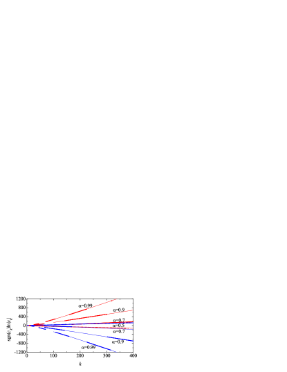
Figure 1: (color online) Plot of $\text{sgn}(c_{k})\ln|c_{k}|$ for $d=3$ and $\alpha=0.5$, $0.7$, $0.9$, and $0.99$. The thin solid lines represent $\pm\left(-k\ln z_{s}-a\ln k+\ln A\right)$, where $a$ and $\ln A$ are fitting parameters.

Figure 2: (color online) Scaled viscosity function $F(z)$ for $d=3$ and $\alpha=0.5$. The thin solid line represents the numerical solution of Eq. (6), while the dashed lines represent the truncated CE expansion $F_{N}(z)$ with $N=5$, $20$, $50$, $100$, and $200$. The thick solid line represents the results obtained from Monte Carlo simulations of the Boltzmann equation AS07 . The steady-state points $(z_{s},F_{s})$ obtained from the kinetic model and the simulations are indicated by the triangle and the circle, respectively. The inset includes $F_{N}(z)$ with $N=1$–$4$ in the region $0\leq z\leq 1.5$.

The first few coefficients $c_{k}$ are listed in Table 1 for $d=3$ and $\alpha=0.5$, $0.7$, $0.9$, $0.99$, and $1$ (elastic hard spheres). As is already apparent from Table 1, the magnitude of the coefficients increases as the system becomes less inelastic, this effect being more and more dramatic with increasing $k$. For instance, the value of $|c_{20}|$ is $1.2\times 10^{-5}$, $5.2\times 10^{-3}$, $2.1\times 10^{5}$, $1.4\times 10^{11}$, and $1.1\times 10^{12}$ for $\alpha=0.5$, $0.7$, $0.9$, $0.99$, and $1$, respectively. Figure 1 shows a log-normal plot of $|c_{k}|$ for the four inelastic systems considered. The results are consistent with an asymptotic behavior of the form $|c_{k}|\approx Ak^{-a}z_{s}^{-k}$, where $z_{s}=\frac{d}{2}\epsilon(1+\epsilon)^{2}$ is the steady-state value of the square uniformity parameter. The exponent $a$ and the amplitude $A$ are estimated by a linear fit of a plot of $\ln(|c_{k}|z_{s}^{k})$ versus $\ln k$ for $100\leq k\leq 400$, the fit being less robust in the case $\alpha=0.5$ than in the other cases. The numerical values of $z_{s}$, as well as of the estimates of $a$ and $\ln A$ are also included in Table 1. In principle, the viscosity function $F(z)$ is different for each dimensionality. However, inspection of Eq. (6) shows that, for a given value of $\epsilon$, the dependence of $F$ on $z$ and $d$ occurs only through the combination $z/d$. Therefore, seen as a function of $\epsilon$ and $z/z_{s}$, $F(z)$ is independent of $d$.

The large-$k$ asymptotic behavior $\ln|c_{k}|\sim-k\ln z_{s}$ for $\alpha<1$ implies that the CE series (1) is convergent for inelastic hard spheres. Moreover, the radius of convergence is $\partial u_{x}/\partial y=\nu z_{s}^{1/2}$ and thus increases with inelasticity. Equation (6) shows that $z=z_{s}$ is indeed a singular point since the steady state $(z_{s},F_{s})$, with $F_{s}=(1+\epsilon)^{-2}$, is the solution of $1-\left(1+\frac{2}{d}zF\right)^{2}F=\epsilon-\frac{2}{d}zF=0$. What is relevant here is that $z=0$ is a regular point (except in the elastic case) and $z=z_{s}$ is the singularity of $F(z)$ in the complex $z$ plane closest to the origin. The convergent character of the series (2) for the most inelastic case considered here ($\alpha=0.5$) is illustrated in Fig. 2, where the numerical solution SGD04 of Eq. (6) is compared with the truncated CE series $F_{N}(z)\equiv\sum_{k=0}^{N}c_{k}z^{k}$ for several values of the truncation order $N$. One can observe that the truncated series agree among themselves and with the numerical solution for $z<z_{s}$. For $z>z_{s}$, however, the CE expansion becomes useless and one must determine $F(z)$ numerically from Eq. (6). An alternative method, successfully used in the elastic case SBD86 , would consist of expanding $F(z)$ around the point at infinity as $F(z)=z^{-2/3}\sum_{k=0}^{\infty}\overline{c}_{k}z^{-k/3}$. Figure 2 also includes results recently obtained from Monte Carlo simulations of the Boltzmann equation AS07 , which show that the predictions of Eq. (6) are quantitatively accurate, even for strong inelasticity, except that Eq. (6) underestimates the location of the steady-state point $(z_{s},F_{s})$. The simulation curve shown in Fig. 2 is the collapse of data obtained by the direct simulation Monte Carlo method starting from 20 different initial conditions (ten for $z<z_{s}$ and ten for $z>z_{s}$), letting the system evolve in time, and discarding the kinetic transients lasting a few mean free times. This explains why the simulation curve does not reach the point $z=0$. For simulation details the reader is referred to Ref. AS07 .

Is the paradoxical regularization by inelasticity of the CE series (1) an artifact of the kinetic model? The following physical argument suggests that this is not the case. Let us assume that the reference homogeneous state is perturbed at time $t=0$ by a weak shear rate $\dot{\gamma}$. Thus the homogeneous state ($\mu=0$) is stable or unstable against this USF perturbation depending on whether the time-dependent uniformity parameter $\mu(t)=\dot{\gamma}/\nu(t)$ asymptotically goes to zero or grows with time. The first situation occurs in a conventional gas of elastic hard spheres since the viscous heating produces a monotonic increase of temperature [cf. Eq. (3) with $\zeta=0$] and thus $\mu(t)\to 0$. However, in a gas of inelastic hard spheres it is always possible that the perturbation is small enough to make the cooling rate prevail over the viscous heating rate and so the temperature keeps decreasing in time [cf. Eq. (3) with $\zeta>0$] until the steady state is eventually reached; thus the uniformity parameter grows, i.e., $\mu(t)\to z_{s}^{1/2}$. Since the CE expansion (2) measures the departure from the reference homogeneous state ($\mu=0$), it is reasonable to expect that the series diverges if $\mu(t)$ goes to zero while it converges if $\mu(t)$ increases with time.

The above heuristic argument can also be applied to the simplest CE series in a compressible flow, namely

$$P_{yy}-nT=-\sum_{k=0}^{\infty}\eta_{k}^{\prime}\left({\partial u_{y}}/{\partial y}\right)^{k+1}.$$ (7)

The full CE expansion of $P_{yy}$ reduces to the series (7) in the uniform longitudinal flow (ULF) characterized by GK96 $\partial u_{y}/\partial y=\dot{\gamma}(t)=\dot{\gamma}_{0}/(1+\dot{\gamma}_{0}t)$ and $n(t)=(n_{0}/\dot{\gamma}_{0})\dot{\gamma}(t)$. The exact energy balance equation, $\partial_{t}T(t)=-({2}/{dn})\dot{\gamma}(t)P_{yy}(t)-\zeta(t)T(t)$, shows that the uniformity parameter $\mu(t)=\dot{\gamma}(t)/\nu(t)$ increases with time if $\dot{\gamma}_{0}>0$, both for elastic and inelastic collisions. However, if $\dot{\gamma}_{0}<0$, $|\mu(t)|\to 0$ in the elastic case whereas $|\mu(t)|$ increases toward a stationary value in the inelastic case. Thus, the CE expansion (7) is expected to diverge for conventional gases and converge for granular gases. This expectation is confirmed by an analysis of the ULF based again on the kinetic model (4).

It is important to note that the dependence on $n$, $T$, and $\alpha$ of the transport coefficients $\eta_{k}$ and $\eta_{k}^{\prime}$ in the partial CE expansions (1) and (7), respectively, is not influenced by the specific state under consideration. Accordingly, the series (1) and (7) converge or diverge irrespective of whether the system is in the USF, the ULF, or in any other state. The advantage of the USF and ULF is that the full CE series of the shear stress and the normal stress reduce to the partial series (1) and (7), respectively, thus allowing us to explore their character in a rather detailed way. Regarding the CE subseries made of linear terms, it is reasonable to expect that, as in the elastic case, it also converges for inelastic collisions, especially if one takes into account the exact mapping between the inelastic and elastic versions of the Enskog–Lorentz equations SD06 .

The CE expansion is the main route to hydrodynamics and so its convergence or divergence has a renewed interest in granular gases in view of some debate on the applicability of hydrodynamics to this class of nonequilibrium systems K99 . I expect that this Letter can contribute to a clarification of this controversial issue by presenting a case study where the application of the CE expansion to describe the nonlinear regime might have a larger practical interest in granular than in conventional gases.

I am grateful to J. W. Dufty and V. Garzó for useful comments on an early version of this paper. This work has been supported by the Ministerio de Educación y Ciencia (Spain) through Grant No. FIS2007–60977 (partially financed by FEDER funds) and by the Junta de Extremadura (Spain) through Grant No. GRU07046.

References

- (1) S. R. de Groot and P. Mazur, Nonequilibrium Thermodynamics (Dover, New York, 1984).
- (2) R. J. Donnelly, “Fluid Dynamics,” in A Physicist’s Desk Reference, ed. by H. L. Anderson (American Institute of Physics, New York, 1989), pp. 196–209.
- (3) S. Chapman and T. G. Cowling, The Mathematical Theory of Non-uniform Gases (Cambridge University Press, Cambridge, 1970).
- (4) H. Grad, Phys. Fluids 6, 147 (1963).
- (5) J. A. McLennan, Phys. Fluids 8, 1580 (1965); G. Scharf, Helv. Phys. Acta 40, 929 (1967); 42, 5 (1969).
- (6) A. W. Lees and S. F. Edwards, J. Phys. C: Solid State Phys. 5, 1921 (1972).
- (7) V. Garzó and A. Santos, Kinetic Theory of Gases in Shear Flows. Nonlinear Transport (Kluwer, Dordrecht, 2003), and references therein.
- (8) A. Santos, J. J. Brey, and J. W. Dufty, Phys. Rev. Lett. 56, 1571 (1986); A. Santos and J. J. Brey, Physica A 174, 355 (1991).
- (9) H. M. Jaeger, S. R. Nagel, and R. Behringer, Phys. Today 49 (4), 32 (1996); Rev. Mod. Phys. 68, 1259 (1996); J. M. Ottino and D. V. Khakhar, Annu. Rev. Fluid Mech. 32, 55 (2000); A. Kudrolli, Rep. Prog. Phys. 67, 209 (2004).
- (10) L. Kadanoff, Rev. Mod. Phys. 71, 435 (1999).
- (11) N. Brilliantov and T. Pöschel, Kinetic Theory of Granular Gases (Oxford University Press, Oxford, 2004); C. S. Campbell, Annu. Rev. Fluid Mech. 22, 57 (1990); J. W. Dufty, J. Phys.: Condens. Matt. 12 A47 (2000); e-print arXiv:0709.0479; I. Goldhirsch, Annu. Rev. Fluid Mech. 35, 267 (2003).
- (12) J. J. Brey, J. W. Dufty, C. S. Kim, and A. Santos, Phys. Rev. E 58, 4638 (1998); V. Garzó and J. W. Dufty, Phys. Rev. E 59, 5895 (1999); Phys. Fluids 14, 1476 (2002); V. Garzó, J. W. Dufty, and C. M. Hrenya, Phys. Rev. E 76, 031303 (2007); V. Garzó, C. M. Hrenya, and J. W. Dufty, Phys. Rev. E 76, 031304 (2007); S. H. Noskowicz, O. Bar-Lev, D. Serero, and I. Goldhirsch, Europhys. Lett. 79, 60001 (2007).
- (13) A. Santos, V. Garzó, and J. W. Dufty, Phys. Rev. E 69, 061303 (2004).
- (14) A. Astillero and A. Santos, Europhys. Lett. 78, 24002 (2007).
- (15) J. J. Brey, J. W. Dufty, and A. Santos, J. Stat. Phys. 97, 281 (1999).
- (16) A. N. Gorban and I. V. Karlin, Phys. Rev. Lett. 77, 282 (1996); I. V. Karlin, G. Dukek, and T. F. Nonnenmacher, Phys. Rev. E 55, 1573 (1997); A. Santos, Phys. Rev. E 62, 6597 (2000).
- (17) A. Santos and J. W. Dufty, Phys. Rev. Lett. 97, 058001 (2006).