Phase diagram and edge effects in the ASEP with bottlenecks

Abstract

We investigate the totally asymmetric simple exclusion process (TASEP) in the presence of a bottleneck, i.e. a sequence of consecutive defect sites with reduced hopping rate. The influence of such a bottleneck on the phase diagram is studied by computer simulations and a novel analytical approach. We find a clear dependence of the current and the properties of the phase diagram not only on the length of the bottleneck, but also on its position. For bottlenecks near the boundaries, this motivates the concept of effective boundary rates. Furthermore the inclusion of a second, smaller bottleneck far from the first one has no influence on the transport capacity. These results will form the basis of an effective description of the disordered TASEP and are relevant for the modelling of protein synthesis or intracellular transport systems where the motion of molecular motors is hindered by immobile blocking molecules.

and

1 Introduction

Driven diffusive systems play an important role in statistical physics. They not only serve as paradigm for non-equilibrium behaviour [1, 2, 3], but also as models for transport processes like vehicular traffic [4], granular flow through narrow pipes [5] and biological transport by motor proteins [6, 7, 8, 9]. The simplest of these models is the totally asymmetric simple exclusion process (TASEP) which was first introduced to describe protein polymerization in ribosomes [10] (for a recent review, see [11]). The TASEP exhibits some generic properties like boundary induced phase transitions [12] that also occur in more complex driven systems. It was solved exactly [13, 14] and results can be used for qualitative and quantitative approaches to other systems. The phase diagram consists of three phases (high density (h), low density (l), and maximum current phase (m)), depending on whether the current is limited by the particle input, output or the transport capacity of the bulk, and is generic for a large class of driven diffusive systems [15].

While homogeneous systems are extensively investigated, systems with inhomogeneous transition rates are not that well understood, especially for the case of open boundary conditions. It is well-known that in nonequilibrium systems even weak disorder can lead to drastic changes [16, 17]. For driven diffusive systems already a single defect site, i.e. a site with reduced hopping rate, can have a global effect on the stationary state, see e.g. [18, 19] for the case of the TASEP with periodic boundary conditions. Here it was shown that in an intermediate density regime $|\rho-1/2|<\rho_{c}$ the current becomes density-independent, i.e. the flow-density relation (fundamental diagram) exhibits a plateau. In contrast, in the limits of low and high densities, the current is unchanged by the presence of the defect.

Here we consider the TASEP with open boundaries in the presence of a bottleneck of length $l$, i.e. a sequence of $l$ consecutive ”slow” bonds, where the hopping rate of the particles is reduced compared to the rest of the system. We will study the effect of such bottlenecks on the phase diagram of the TASEP, focussing on the maximal current that can be maintained by the system through optimization of the input and output rates, i.e. its transport capacity.

In open systems, the main effect of the bottleneck (or defects in general) is a decrease of the transport capacity [20]. This leads to an enlarged maximum current phase compared to the pure system. In addition the density profiles in the maximum current phase exhibit phase separation into a high density and low density regime separated by a shock.

The effect of defects in systems with open boundaries has been studied earlier by several authors. So far no exact solutions are known and one has to rely on computer simulations with Monte Carlo (MC) methods and mean-field type approximations.

Kolomeisky [20] investigated the TASEP in the presence of a single defect site ($l=1$) deep in the bulk. Analytical results are obtained by a mean field approach which neglects correlations on the slow bond by dividing the system into two homogeneous ones coupled at the defect site. Therefore this approach is limited to single defect sites ($l=1$). Comparison with MC results shows a good agreement, at least for the high- and low-density phases. The mean field treatment also leads to deviations of density profiles near the defect site from the MC results.

In [21], Chou and Lakatos gave an analytical approach treating a finite number of bottlenecks of arbitrary lengths. Their finite segment mean field theory (FSMFT) divides the system into segments which contain one or a few defect sites. By determining the leading eigenvector of the corresponding transition matrix and matching the currents of the different subsystems, predictions for the current through the system are obtained which at the same time take into account correlations near the bottlenecks. Although the method allows to treat several defect sites of arbitrary hopping rates within the segment, it is restricted to segment lengths of less than 20 sites due to the numerical complexity.

The results for one and two defect sites ($l=1$) in the bulk were recently extended by Dong et al. [22]. Additionally they have considered the case where a single defect is located near the boundary of the system and found an edge effect induced by the interaction of this defect with the boundary. This implies a dependence of the current on the position of the defect. Finally, the effects of Langmuir kinetics, i.e. particle-creation and -annihilation in the bulk have been shown [23] to lead to a rich phase diagram including novel phases.

The present investigation generalizes the previous works in several aspects. Especially we will study systematically the dependence of the current on the length $l$ of the bottleneck and its position. For this purpose we develop an analytical approach to calculate the current and critical boundary rates, called the interacting subsystem approximation (ISA). Mathematically it requires finding a specific root, constrained by physical requirements, of a polynomial which has a degree of order $l$. For longer bottlenecks this approach is more efficient than the approach of [21] which demands to search an eigenvector of a $2^{l}\times 2^{l}$-matrix. This allows us to generalize the single defect results of Dong et al. [22] to longer bottlenecks. The increase of the maximum current by moving defects near the boundary is reproduced by ISA and extended to the case $l>1$ (positive edge effect). However, for lower entry rates ISA predicts a decrease of the current (negative edge effect) which is confirmed by MC simulations. We also observe in MC simulations an intermediate regime which shows a non-monotonic dependence of the current on the position of the bottleneck. Furthermore we conclude that for bottlenecks near the boundaries there is no phase transition to a maximum current phase, since the current is not constant in any regime, but it approaches the maximum current asymptotically for higher entry and exit rates, and there is no macroscopic phase separation.

We also consider the case of two bottlenecks of arbitrary lengths and separation generalizing the corresponding results of [22] for two single defects. Therefore we also investigate the case that one of the bottlenecks is near the boundaries. The results will motivate a concept of effective boundary rates that encompasses the effect of boundary-near bottlenecks. This provides the basis for an extensive study [24] of finite defect densities, i.e. a macroscopic number of slow bonds. Here previous investigations for periodic [25, 26, 27, 28] and open systems [28, 29, 30, 31, 32, 33] have revealed surprising results. For the open system, for example, it has been found [30] that the position of the phase transitions is sensitively sample-dependent even for large systems.

2 Definition of the model

We consider a TASEP consisting of $L$ sites which can either be empty or occupied by one particle. Throughout this paper we are mainly interested in the steady-state in the limit $L\to\infty$. With each bond between neighbouring sites $j$ and $j+1$ we associate a hopping rate $p_{j,j+1}$ which corresponds to the rate at which a particle will move from $j$ to its right neighbour $j+1$ if this is empty. At the boundary sites $j=1$ and $j=L$ particles can be inserted and removed, respectively. If site $1$ is empty a particle will be inserted there with rate $\alpha$. On the other hand, if site $L$ is occupied this particle will be removed with rate $\beta$. Here we will use a random-sequential update corresponding to continuous-time dynamics.

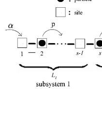
Figure 1: Illustration of the TASEP with a bottleneck of length $l$, i.e. $l$ consecutive defect bonds (or sites resp.). The defect bonds/sites are characterized by a hopping rate $q<1$, whereas at the other bonds/sites the hopping rate is $p=1$. The system is virtually divided into three subsystems with virtual entry/exit rates corresponding to the mean occupation/vacancy on the adjacent sites.

In this paper we study the effect of a single bottleneck of length $l$, i.e. a section of $l$ consecutive slow bonds (or sites) with hopping rate $p_{j,j+1}=q<1$ (Fig. 1). All other bonds are fast bonds with hopping rate $p_{j,j+1}=1$.

In order to determine relevant quantities like the current and critical boundary rates, we approach the problem by virtually dividing the system into three interacting subsystems (Fig. 1): A system of $L_{1}$ sites with hopping rate $p_{j}=1$ at the left end of the chain, a section of length $L_{2}=l+1$ consisting of the bottleneck with $l$ slow sites (hopping rate $q$) extending from site $s=L_{1}+1$ to site $L_{1}+l=L_{1}+L_{2}-1$ plus an extra fast site $f=L_{1}+L_{2}$ at the right end, and finally another pure system of length $L_{3}$ with hopping rates $p_{j}=1$. Note that subsystem 2, which contains the bottleneck, starts and ends with a fast bond. This symmetry of the subsystem will be more convenient for our investigations.

The main idea of our approach is to use the exact solution for the stationary state of the pure TASEP with random-sequential dynamics [13, 14]. This solution applies to all three pure subsystems defined above. The interactions between these subsystems are described by suitably chosen boundary rates. We neglect correlations at the sites connecting the subsystems. Introducing the occupation number $\tau_{j}=0,1$ of site $j$, this explicitly means that we assume

$$\langle\tau_{j}(1-\tau_{j+1})\rangle\approx\rho_{j}(1-\rho_{j+1})\qquad{\rm for\ }j=s-1,f$$ (1)

where $\rho_{j}:=\langle\tau_{j}\rangle$ is the average local density at site $j$. This approach is similar in spirit to that of Kolomeisky [20] for the case of a single defect ($l=1$). However, there correlations on the slow bond are neglected whereas here we will treat the bottleneck also as a pure system (of reduced hopping rate) so that the most relevant correlations induced by it are taken into account. The three subsystems are coupled through virtual boundary rates $\alpha_{j}$, $\beta_{j}$. Note that all these rates are associated with fast bonds. In the following we will call this approach the interacting subsystem approximation (ISA) to distinguish it from the usual mean-field approach which neglects all correlations.

The rate equations at the sites connecting the subsystems are then given by

$$\frac{d}{dt}\langle\tau_{s-1}\rangle=\langle\tau_{s-2}(1-\tau_{s-1})\rangle-\beta_{1}\langle\tau_{s-1}\rangle\,,$$ (2)

$$\frac{d}{dt}\langle\tau_{s}\rangle=\alpha_{2}(1-\langle\tau_{s}\rangle)-q\langle\tau_{s}(1-\tau_{s+1})\rangle\,,$$ (3)

and

$$\frac{d}{dt}\langle\tau_{f}\rangle = q\langle\tau_{f-1}(1-\tau_{f})\rangle-\beta_{2}\langle\tau_{f}\rangle\,,$$ (4)

$$\frac{d}{dt}\langle\tau_{f+1}\rangle = \alpha_{3}(1-\langle\tau_{f+1}\rangle)-\langle\tau_{f+1}(1-\tau_{f+2})\rangle\,,$$ (5)

with the virtual boundary rates

$$\alpha_{2}=\rho_{s-1}\,,\qquad\alpha_{3}=\rho_{f}\,,\qquad\beta_{1}=1-\rho_{s}\,,\qquad\beta_{2}=1-\rho_{f+1}\,,$$ (6)

in terms of the average local density $\rho_{j}$. For completeness, we also define $\alpha_{1}:=\alpha$ and $\beta_{3}:=\beta$. Note that the mean-field factorization of expectation values only applies to the sites at the boundaries of the subsystems. All correlations within the subsystems will be taken into account exactly!

From the exact solution of the TASEP with $N$ sites for hopping rate $p=1$, we know the “partition function” [13]

$$\mathcal{Z}(\alpha,\beta,N)=\sum_{\{\tau_{i}=0,1\}}\mathcal{P}(\{\tau_{i}\})=\sum_{j=1}^{N}\frac{j(2N-1-j)!}{N!(N-j)!}\frac{(1/\beta)^{j+1}-(1/\alpha)^{j+1}}{(1/\beta)-(1/\alpha)},\quad\,$$ (7)

which is exact for all system sizes $N\geq 1$. Here $\mathcal{P}(\{\tau_{i}\})$ is the probability of finding the stationary system in a configuration $\{\tau_{i}\}$. The singularity at $\alpha=\beta$ can be removed by taking the limit $\alpha\to\beta$ which yields the analytic continuation

$$\mathcal{Z}(\alpha,N):=\lim_{\beta\to\alpha}\mathcal{Z}(\alpha,\beta,N)=\sum_{j=1}^{N}\frac{j(2N-1-j)!}{N!(N-j)!}(j+1)\left(\frac{1}{\alpha}\right)^{j}\,.$$ (8)

The corresponding results for the TASEP with hopping rate $p\neq 1$ can be obtained by rescaling of the boundary rates $\alpha\to\alpha/p,\,\beta\to\beta/p$. Thus the partition function in a pure TASEP with hopping rate $p$ is

$$\mathcal{Z}_{p}(\alpha,\beta,N)=\mathcal{Z}\left(\frac{\alpha}{p},\frac{\beta}{p},N\right)\,.$$ (9)

This result will be used in the following for different values of $N$, depending on the length of the subsystems.

The exact current $J_{0}$ of a pure system of length $N$, which is the quantity most relevant in the following, can be expressed through the partition function as [13]

$$J_{0}(\alpha,\beta,N)=\frac{\mathcal{Z}(\alpha,\beta,N-1)}{\mathcal{Z}(\alpha,\beta,N)}\,.$$ (10)

Conservation of current then yields the central equations of the ISA

$$J_{0}(\alpha_{1},\beta_{1},L_{1})=J_{0}\left(\frac{\alpha_{2}}{q},\frac{\beta_{2}}{q},L_{2}\right)=J_{0}(\alpha_{3},\beta_{3},L_{3})$$ (11)

which express the fact that the current in the stationary state is the same in all three interacting subsystems. Note that we have used (9) and (10) to express the current in the bottleneck (subsystem 2) through the result $J_{0}$ for a pure system.

Inserting (7) and (10) in (11) we obtain a set of two algebraic equations with six variables. In principle one can solve these equations, if four of the variables are known or more equations are given that determine variables.

3 One bottleneck far from the boundaries

First we study the case where the bottleneck is far from the boundaries. So we assume that $L_{1}$ and $L_{3}$ are large. From the latter condition it is expected that the topology of the phase diagram is the same as that of a system with a single defect ($l=1$). We can therefore follow [20] and classify the phases by the phases of the pure subsystems 1 and 3 which are ${\mathcal{O}}(L)$.

Though at first glance one could expect nine possible phases corresponding to all possible combinations of three phases l,h,m (see Sec. 1) that can be realized in the pure subsystems 1 and 3, it was argued in [20] that only the combinations l-l, h-h and h-l can exist. The l-l-phase corresponds to a global low density phase (L), while h-h corresponds to a high density phase (H). In both cases, only around the bottleneck there are local deviations from the density profile of the homogeneous system. In the h-l-phase, we have phase separation which cannot be observed in the pure system. The current in the h-phase is independent of the entry rate, while in the l-phase it is independent of the exit rate. Thus in a phase separated h-l-phase, the current is independent of both boundary conditions and takes a maximum value (see below). Although it is sometimes called a maximum current phase (M) like in the pure system, its properties differ from the maximum current phase in the pure system not only by the occurrence of phase separation, but also by the absence of algebraic boundary layers. Therefore we prefer the terminology phase separated regime (PS). Furthermore, the transition to this phase corresponds to a transition of subsystem 1 from l to h and vice versa respectively, which is accompanied by a discontinuity of the mean density $\langle\rho\rangle=\sum_{j}\rho_{j}$. According to this, it can be classified as a first order transition in contrast to the pure system where the transition to the maximum current phase is of second order.

Though the system with a bottleneck is not exactly invariant under the particle-hole symmetry operation defined by $\tau_{j}\leftrightarrow 1-\tau_{j},\,\alpha\leftrightarrow\beta,\,j\leftrightarrow L-j$, this transformation only changes the position of the bottleneck, but still leaves it far from the boundary. Thus the particle-hole transformation leaves the phases of the subsystems unchanged, since it only changes their sizes, but they stay ${\mathcal{O}}(L)$. Therefore, we can conclude that the phase diagram must be symmetric with respect to the line $\alpha=\beta$. This symmetry constraint yields that the transition line between high and low density phase must be at $\alpha=\beta$.

We now want to determine the critical entry rate $\alpha^{*}$ at the transition from the L-phase to the PS-phase for fixed $\beta$ in terms of the analytical ISA approach introduced in the last section. It corresponds to the transition of (the pure) subsystem 1 from low to high density phase which occurs at $\alpha^{*}=\alpha_{1}=\beta_{1}$. Furthermore we know that at this point $J=\alpha_{1}(1-\alpha_{1})$. Subsystem 3 still remains in the low density phase. Therefore we also have $J=\alpha_{3}(1-\alpha_{3})$. Since the current must be the same as in subystem 1 and $\alpha_{3}$ must be smaller than 1/2 we conclude $\alpha_{3}=\alpha^{*}$. From the definition of the virtual boundary rates (2), (6) we obtain by a simple transformation

$$\beta_{2} = J/\rho_{f}=J/\alpha^{*}=1-\alpha^{*}\,,$$ (12)

$$\alpha_{2} = J/(1-\rho_{s})=J/\beta_{1}=J/\alpha^{*}=1-\alpha^{*}\,,$$ (13)

where the first equality in each equation can be found e.g. in [13]. From the exact solution of the pure TASEP (10), (7) and the conservation of current (11), it follows

$$J\left(\frac{1-\alpha^{*}}{q},\frac{1-\alpha^{*}}{q},l+1\right)=\alpha^{*}(1-\alpha^{*})$$

$$\Longleftrightarrow\hskip 14.22636pt \alpha^{*}(1-\alpha^{*})\mathcal{Z}((1-\alpha^{*})/q,l+1)=\mathcal{Z}((1-\alpha^{*})/q,l)\,,$$ (14)

where $\mathcal{Z}(1-\alpha,l+1)$ is the limit defined in (8) and $\mathcal{Z}(1-\alpha,l+1)\neq 0$ for $0\leq\alpha\leq 1$.

Eq. (3) is essentially a polynomial in $1/\alpha^{*}$ (or $\alpha^{*}$, respectively) and can be solved numerically (or analytically for small values of $l$). The requirement that a physical relevant solution for $\alpha^{*}$ has to be in the interval $[0,\frac{1}{2}]$ gives a unique solution $\alpha^{*}(q,l)$ for the transition point to the PS-phase. In general, the solution depends on the length $l$ of the bottleneck and the slow hopping rate $q$. For $l=1$, for example, equation (3) can be transformed into

$$2{\alpha^{*}}^{2}-(2+3q)\alpha^{*}+2q=0\,.$$ (15)

The relevant solution is then

$$\alpha^{*}=\frac{2+3q}{4}-\sqrt{\frac{(2+3q)^{2}}{16}-q}\,.$$ (16)

Explicitly, for the value $q=0.6$ used in most simulations, one obtains $a^{*}=\frac{2}{5}$ by evaluating (16).

The current at the transition point corresponds to the maximum current $J^{*}$ in the PS-phase which can be interpreted as the transport capacity of the system. From (3) we can see that

$$J^{*}(q,l)=\alpha^{*}(q,l)(1-\alpha^{*}(q,l))\,,$$ (17)

which yields $J^{*}(0.6,1)=\frac{6}{25}$ for $q=0.6$ after taking into account (16).

In Fig. 2 we have plotted the dependence of $J^{*}(q,l)$ on the slow hopping rate $q$ (for fixed $l$) obtained by (17) and compare these analytical ISA-results with results from Monte Carlo (MC) simulations for different bottleneck lengths. For a single defect site ($l=1$) we have compared the analytical results obtained by (16) and (17) with the results obtained by pure mean field approximation $J^{*}_{MF}=\frac{q}{(1+q)^{2}}$ [20]. Obviously also for $l=1$ the results obtained by (17) are more accurate than mean field results, while for longer bottlenecks, to our knowledge, no proper mean field approximations are known. Note that our approximation takes into account correlations on the slow bonds, only correlations on sites adjacent to the bottleneck are neglected.

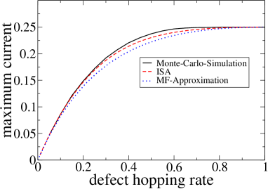
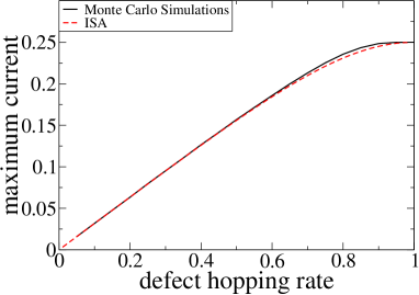
Figure 2: Maximum current in a system with a bottleneck far from the boundaries in dependence on the slow hopping rate $q$. It is determined by Monte Carlo simulations for $\alpha=\beta=0.5$ and by solving the ISA equation (3) for a bottleneck of length $l=1$ (left) and $l=6$ (right). For comparison the mean field approximation $J^{*}_{{\rm MF}}=\frac{q}{(1+q)^{2}}$ for $l=1$ is included.

Fig. 3 shows the maximum current in dependence of the bottleneck length $l$. Here we compare MC-simulations with the results obtained by (17). The ISA results systematically underestimate the real current. The deviation is largest for small $l$, but it does not exceed 3%. For larger bottlenecks, the agreement improves. We also note that we have chosen $q=0.6$ since for this value the observed deviations have been found to be largest. In addition we plotted the exact current of the pure system with system size $L=l+1$ and $\alpha=\beta=1$. It seems that the asymptotics for large $l$ are the same as for the bottleneck.

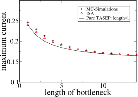
Figure 3: Maximum current in dependence of the bottleneck size for $q=0.6$. MC-simulations are compared with ISA results. The solid line is the current in a homogeneous TASEP with $L=l+1$,  $\alpha=\beta=1$ and hopping rate $q=0.6$.

In Fig. 4 the dependence of the mean density $\langle\rho\rangle=\frac{1}{L}\sum_{i=1}^{L}\rho_{i}$ and the current $J$ on the entry rate $\alpha$ is plotted for fixed $\beta$. In order to compute these quantities, we used the method introduced in [30] that allows to calculate the current and densities for an arbitrary set of values of $\alpha$ in one simulation. One observes a steep increase of the mean density for the same value of $\alpha$ where the maximum current plateau begins. This seems to coincide with the value of $\alpha^{*}$ obtained by ISA quite well. The slope increases with system size indicating a discontinuity in the thermodynamic limit corresponding to a first order phase transition, in contrast to the pure TASEP. The plots also show that at the transition point and in the hole PS-phase, the current is maximal.

As we have argued above, the phase diagram must be symmetric with respect to the diagonal $\alpha=\beta$ that yields $\beta^{*}=\alpha^{*}$. With this information we can sketch the phase diagram of the TASEP with one bottleneck far from the boundaries displayed in Fig. 4. Its topology is the same as the one for a single defect far from the boundaries [20], while longer bottlenecks have a larger PS-phase than single defects. It also looks similiar to the phase diagram of the pure TASEP but here all phase transitions are of first order in contrast to the TASEP and the characteristics of the M-phase and PS-phase are different.

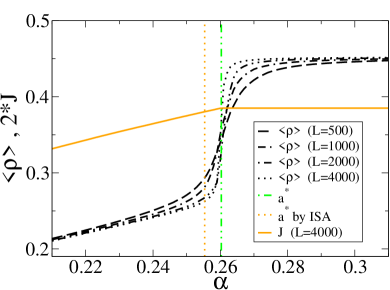
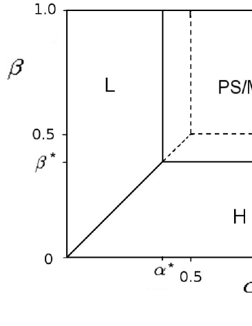
Figure 4: Left: Mean density $\langle\rho\rangle$ and current $J$ as function of $\alpha$. The slope of $\langle\rho\rangle(\alpha)$ becomes steeper for larger systems indicating a discontinuity in the thermodynamic limit. The vertical lines show the steepest point of $\langle\rho\rangle(\alpha)$ identified as the phase transition $\alpha^{*}$ compared with the ISA results from (3).
Right: Schematic phase diagram of the TASEP with one bottleneck far from the boundaries. It looks similiar to the phase diagram of the pure TASEP while the transition lines to the maximum current (phase separated) phase is shifted to be at $\alpha^{*}$ and $\beta^{*}$. The mean density is discontinuous at these points.

Another procedure to compute the maximum current for a finite bottleneck is the finite segment mean field theory (FSMFT) introduced in [21]. In this approach, a segment of $l^{\prime}$ sites including the bottleneck of length $l<l^{\prime}$ is considered. Currents can then be obtained from the eigenvector of the zero-eigenvalue of the $2^{l^{\prime}}\times 2^{l^{\prime}}$-transition matrix of this segment [21]. The advantage of this method is that the accuracy can be systematically increased by expanding the size $l^{\prime}$ of the segment. It can also treat arbitrary combinations of hopping rates inside the segment. However, due to the exponentially decreasing size of the transition matrix one is currently restricted to segment lengths $l<20$. In contrast, the ISA-method, though not asymptotically exact, relies on finding one specific root of a polynomial equation of a maximal degree $l+2$. This makes it possible to compute the maximum current for systems with large bottlenecks of several hundred sites rather easily. This advantage becomes relevant for disordered systems with finite defect site density where bottlenecks of arbitrary length can occur. For example the computation of the maximum current of a system with 500 consecutive defect sites can be made in less than one second on a standard PC to obtain $J^{*}_{ISA}(l=500)=0.15045$ for $q=0.6$. Although this agrees nicely with the value from MC simulations, $J^{*}_{MC}=0.15049$, it is clearly different from the asymptotic value $J^{*}_{\infty}=q/4=0.15$ for $l\to\infty$ [27, 25, 21].

4 Edge effects: One bottleneck near a boundary

Next we consider a system with a bottleneck near the left boundary, i.e. now both $L_{1}$ and $L_{2}=l+1$ are of order $\mathcal{O}(1)$ for $L\to\infty$. The case of a bottleneck at distance $d$ from the right boundary, i.e. the last slow site is at site $L-d-1$, has not to be considered separately since we can deduce the results using the particle hole-symmetry

$$\alpha\leftrightarrow\beta,\,\,\,\rho_{j}\leftrightarrow 1-\rho_{j}\,,\,\,\,j\leftrightarrow L-j,\,\,\,\mbox{subsystem 1}\leftrightarrow\mbox{subsystem 3}\,.$$ (18)

Since we have only one macroscopic subsystem, namely subsystem 3, the classification of phases is slightly different than in Sec. 3. Now the phase of the system with bottleneck is basically identically to that of subsystem 3. Phase separation can no longer occur since the size of subsystem 1 is microscopic. The entry rate $\alpha_{3}$ of subsystem 3, defined in ISA (see (2)-(5)), can thus be treated as an effective entry rate $\alpha_{\mathrm{eff}}:=\alpha_{3}\neq\alpha$ for the bulk of the system which is a homogeneous TASEP. The phase of the full system corresponds to the phase of subsystem 3 which we now denote by L’, H’ or M.

For $L_{1}\geq 2$, we can divide the system into three subsystems in the same manner as in Fig. 1. First we consider a system in the low-density phase L’. Therefore the current is given by

$$J=\alpha_{\mathrm{eff}}(1-\alpha_{\mathrm{eff}})\,.$$ (19)

In the steady state the entry and exit rates of a pure TASEP with $N$ sites are $\alpha=\frac{J}{1-\rho_{1}}$ and $\beta=\frac{J}{\rho_{N}}$ [13]. The currents in subsystems 1 and 2 have to be identical and thus, as in (11),

$$J_{0}(\alpha,1-\rho_{s},L_{1}) = J_{0}\left(\frac{J}{q(1-\rho_{s})},\frac{J}{q\rho_{f}},L_{2}\right)\,,$$ (20)

where $J_{0}$ is the exact current in a pure system given by (10) and $\rho_{s}$ and $\rho_{f}$ are defined in the same manner as in Sec. 3. Since subsystem 3 is assumed to be in the low density phase, the density profile is flat at its left end, i.e. the density is independent of the position if we apply ISA. Therefore we have $\alpha_{\mathrm{eff}}=\rho_{f}=\rho_{f+1}$ and can take $J=\rho_{f}(1-\rho_{f})$ in eq. (20). Furthermore the currents in subsystem 1 and subsystem 3 have to be the same which leads to

$$J_{0}(\alpha,1-\rho_{s},L_{1})=\rho_{f}(1-\rho_{f})\,.$$ (21)

Now we have two ISA-equations, (20) and (21), as well as the two variables $\rho_{s}$ and $\rho_{f}=\alpha_{\mathrm{eff}}$. For given $\alpha$, $L_{1}$ and bottleneck length $l$ these equations can be solved to obtain the effective entry rate $\alpha_{\mathrm{eff}}$, while the resulting current can be obtained from (19).

For $L_{1}=1$ that procedure does not work in the same way because the current in a system of size 1 is not defined as one can see in (10). But even in this case, we still have $\alpha=J/(1-\rho_{1})$ which is valid by definition of the boundary rates. After inserting $J=\rho_{f}(1-\rho_{f})$, this equation together with (21) again gives a solvable set of two equations with the two variables $\rho_{s}$ and $\rho_{f}$.

For $L_{1}=0$ subsystem 1 does not exist and we have only the two subsystems 2 and 3. Subsystem 2 comprises the sites $\{1,\ldots,L_{2}\}$ and subsystem 3 $\{L_{2}+1,\ldots,L\}$ which includes the bulk of the system. This problem can however be solved, by inserting

$$\alpha_{2}=\alpha\,,\qquad\beta_{2}=\frac{J}{1-\rho_{f}}\,,\qquad\alpha_{3}=\rho_{f}\,.$$ (22)

Analogous to (11) we thus obtain the equation

$$J_{0}\left(\frac{\alpha}{q},\frac{J}{q(1-\rho_{f})},L_{2}\right)=\rho_{f}(1-\rho_{f})\,,$$ (23)

with $J=\rho_{f}(1-\rho_{f})$. This equation can be solved for the variable $\rho_{f}=\alpha_{\rm eff}$ thus we obtain the effective entry rate and by (19) the corresponding current.

Because of the particle-hole symmetry (18) we can transfer these results for $\beta_{{\rm eff}}$ in the high-density phase. The effective exit rate for the bulk $\beta_{{\rm eff}}$ can then be determined using (19)-(23). Note that in the low-density phase, $\beta$ has no influence on the bulk of the system, only in a small region near the boundaries. The same is valid in a high-density phase for $\alpha$.

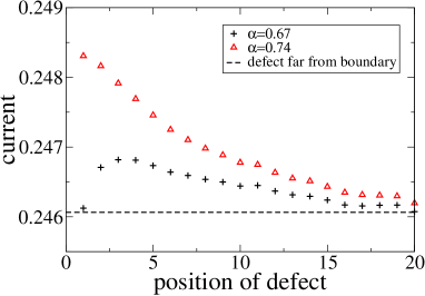
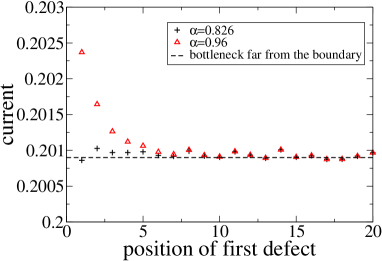
Figure 5: Current in a system with a single defect site (left) and a bottleneck of length $l=4$ (right) near the left boundary in dependence on its position, for high entry rates. The exit rate is $\beta=1.0$. The system size is $L=500$ while the number of iterations is 40000000, $q=0.6$. The entry rates have been chosen in order to optimally display the mixed and the positive edge effect. In the system with the longer bottleneck (right), the mixed edge effect is almost not visible even for optimized parameters. Note that the magnitude is much smaller than in Fig. 6.

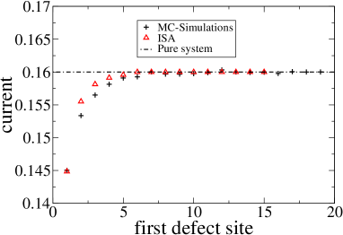
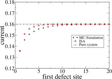
Figure 6: Current in a system with a bottleneck near the boundaries in dependence of the position of the first defect site, for low entry rates. The exit rate is $\beta=\alpha$, system size $L=500$ and number of MC steps $=2000000$ for bottleneck length $l=1$, $q=0.6$, and $\alpha=0.2$ (left), bottleneck length $l=4$, $q=0.6$ and $\alpha=0.2$ (right). The scale for the current has been chosen in order to emphasize the form of the deviations.

4.1 Edge effect: discussion

In Fig. 5 and 6 we have plotted the current in dependence on the position of the first defect site for different values of $\alpha$ while $\beta=1$. One observes that the position of the bottleneck has a significant influence on the current. This is called the edge effect, first observed in [22]. In that work only an increase of the current was observed if defects approach the boundary (positive edge effect) which can be seen in Fig. 5. In addition, ISA predicts a decrease of the current for low entry rates. This negative edge effect is confirmed by MC simulations (Fig. 6). There is also a region of entry rates, where the dependence of the current on the bottleneck position is non-monotonic (mixed edge effect, see Fig. 5)! Simulations for different system sizes indicate that this non-monotonic behaviour is not a finite-size effect. Nonetheless, as we can also see in the figures, the magnitude of the positive and the mixed edge effect is much smaller than the one of the negative edge effect. The ISA results obtained from the equations in the last subsection confirm the existence of negative and positive edge effect, while the mixed one is not. This indicates that the mixed edge effect is caused by correlations at the edge of the bottleneck. In Fig. 6 we plotted the analytical results for comparison. We did not display them in Fig. 5 since the deviations due to correlations are larger than the positive/mixed edge effect itself. In the appendix it is shown that the negative edge effect is predominant in regimes where the current depends significantly on the boundary rates.

Moreover, we see that the current does not attain a plateau value. Instead it seems to approach asymptotically the value $J=0.25$ (Fig. 7). This is confirmed by our simulations, where we calculated the current for the very high value $\alpha=100$ that yielded an effective entry rate of $\alpha_{\rm eff}\approx 0.5$. Since we assume the effective entry rate to grow monotonic with the real entry rate, we can conclude that we have always $\alpha_{\rm eff}<0.5$, thus the maximum current phase can never be attained. As we have argued above, there is no phase separation, either, if the distance of the bottleneck from the boundary is microscopic, so we can state that for a bottleneck near the boundary only the high and low density phase can occur. This is plausible since a similar argument for the absence of the maximum current phase in subsystem 3 as in Sec. 3 applies.

Though strictly speaking there is no M/PS-phase if the bottleneck is near a boundary, the system still exhibits a kind of crossover. While there is neither a plateau region nor a sharp kink in the dependence of the current on the entry rate (see Fig. 7), for higher entry rates this dependence is rather weak. For a bottleneck far from the boundaries we actually have sharp phase transitions, so we can say that by approaching the bottleneck to the boundary, the phase transition to the M/PS-phase is “softened” into a crossover.

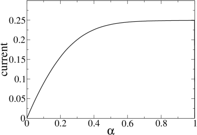
Figure 7: Current in dependence on the entry rate $\alpha$ for $\beta=1$ and a defect at site $j=3$. Results are obtained by MC simulations. There is no plateau.

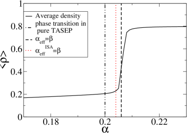
Figure 8: Average density in dependence on the entry rate for $\beta=0.2$ and a defect at site 3. The transition to the high density phase is shifted to larger $\alpha$ compared to the pure system.

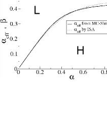
Figure 9: Effective entry rate in dependence on $\alpha$. Interpreting the y-axis as the beta range, this corresponds to the phase diagram with the graph being the transition line between H-phase (below) and L-phase (above).

The transition from low density phase to the high density phase occurs for $\beta=\alpha_{\rm eff}$. This is confirmed in Fig. 8 where we have plotted the average density in dependence on $\alpha$. The jump in the average density marks the transition point, which matches quite good the value of $\alpha_{\rm eff}$. One observes that the transition point is shifted to higher values of $\alpha$ compared to the transition in the pure system $\alpha=\beta$. In this diagram, $\alpha_{\rm eff}$ was obtained by the formula $\alpha_{\rm eff}=\frac{J}{1-\rho_{f+1}}$. The value calculated by solving the ISA equations (20) and (21) is a little less, but it still yields the correct sign of the shift of the transition point.

Fig. 9 shows the dependence of $\alpha_{\rm eff}$ on $\alpha$. Since $\beta=\alpha_{\rm eff}$ is the transition line between high and low density phase, the diagram simultaneously displays the phase diagram, interpreting the y-axis as the $\beta$-range. As we see the phase transition line calculated in ISA is in good agreement with MC results.

5 Two bottlenecks far from the boundaries

The next step towards disordered systems is the investigation of a system with two bottlenecks. This will tell us something about the importance of ”interactions” between the bottlenecks. We distinguish two cases. First we will consider situations where both bottlenecks are in the bulk of the system, i.e. far away from the boundaries. Then we study edge effects in more detail by allowing one bottleneck to be close to one of the boundaries. Unfortunately, we cannot use the analytic ISA approach applied in the last sections since the equations would be underdetermined. Thus we have to rely on simulation results.

5.1 Two bottlenecks far from the boundaries

We simulated systems with two bottlenecks of length $l_{1}$ and $l_{2}$ with $d$ fast sites in between. We focussed on the maximum current phase and determined the current $J^{*}_{2}$. In Fig. 10, $J^{*}_{2}$ is plotted as function of the distance $d$ between the bottlenecks for different values of $l_{1}$ and $l_{2}$. One sees that, if the lengths of the two bottlenecks differ with $l_{1}>l_{2}$, $J^{*}_{2}$ tends to converge to $J^{*}(l_{1})$, which is the value obtained in a system with only the longer bottleneck. The convergence is faster for a larger difference $l_{1}-l_{2}$ of the bottleneck lengths. In this case for a distance of about 5-10 lattice sites, the maximum current is almost the same as for a system with only the longer of the two bottlenecks. Of course for $d\to 0$ the bottlenecks merge, thus we have only one bottleneck and $J^{*}_{2}(l_{1},l_{2},0)=J^{*}(l_{1}+l_{2})$. If both bottlenecks have equal size, $d\to\infty$ converges to the maximum current of a single bottleneck which generalizes results of [22] to the case $l_{1}=l_{2}>1$.

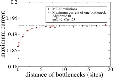
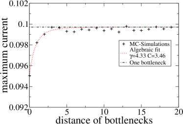
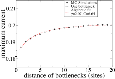
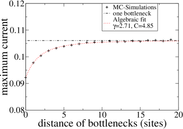
Figure 10: Maximum current in a system with two bottlenecks of length $l_{1}$ (the first one) and $l_{2}$ (the second one) far from the boundaries in dependence on the distance of the two defects. The current is determined by MC simulations for $\alpha=\beta=0.5$. In each graph an algebraic fit of the form $f(d)=J^{*}(l_{1})-(d+C)^{-\gamma}$ with fit parameters $C$ and $\gamma$ is included. $J^{*}(l_{1})$ is obtained from the MC simulations in Sec. 3. One observes, that the maximum current converges to the maximum current of a system with a single bottleneck, i.e. the longer one. The parameters are $l_{1}=5$, $l_{2}=1$, $q=0.6$ (top left), $l_{1}=5$, $l_{2}=1$, $q=0.3$ (top right), $l_{1}=4$, $l_{2}=3$, $q=0.6$ (bottom left), and $l_{1}=4$, $l_{2}=3$, $q=0.3$ (bottom right).

5.2 Two bottlenecks: Edge effects

Next we simulated a system with two bottlenecks where one is near the boundary and one is far away. We concentrated on the case, where the bulk bottleneck is larger than that close to the boundary.

In Fig. 11, we plotted the dependence of the current on the distance of the first bottleneck. For comparison we included the results for a single bottleneck near the boundary from section 4. One observes no significant difference between the two datasets. This observation indicates that bottlenecks far from the boundary do not have any influence on the current, as long as the current is below the maximum current allowed by that bottleneck.

In Fig. 12, however, we see the maximum current in a system with a bottleneck of length $l$ far from the boundaries and a defect at site 3. Again, one does not see a significant difference: a small bottleneck near the boundary has no influence on the transport capacity.

In agreement with observations already made in [21], our results motivate the view of a local influence of bottlenecks that yields the possibility to generalize concepts of the TASEP with single bottleneck to systems with many bottlenecks. Only bottlenecks near the boundaries have influence on the current if it is below the transport capacity. We therefore propose that the influence of boundary defects can be taken into account through effective boundary rates in the same manner as for a single bottleneck near the boundaries. That means that below the maximum current we can describe the system as a pure TASEP, but with effective boundary rates $\alpha_{\rm eff},\beta_{\rm eff}$ depending on the configuration of bottlenecks near the boundaries instead of the pure ones.

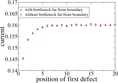
Figure 11: Dependence of the current on the position of the first defect for $\alpha=0.2$ and $\beta=1.0$. Comparison of a system with only one defect and a system with a additional bottleneck far from the boundaries.

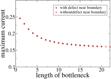
Figure 12: Maximum current in dependence on the bottleneck length for $q=0.6$. The addition of a defect near the boundaries does not alter the maximum current.

6 Discussion and Outlook

We have investigated the TASEP in the presence of a bottleneck of $l$ consecutive slow sites. Apart from computer simulations we have developed an approximate analytical approach called interacting subsystem approximation (ISA) that makes use of the exact results obtained for the pure TASEP. ISA turns out to be an efficient and accurate method for systems with a single bottleneck. It can be applied to other systems as long as exact results are available.

Therefore we have divided the system into subsystems consisting of fast and slow sites only, where the exact solution [13, 14] for the homogeneous system applies. In the treatment of the coupling of these systems certain correlations are neglected. Nevertheless the predictions of the analytical approach are in good agreement with the simulations, while they slightly underestimate the real current. Our method yields much better results than e.g. the mean field approach in [20] for single defects. For longer bottlenecks it is much more computationally efficient than the approach by Chou and Lakatos [21], which produces results of a similar accuracy. The finite segment mean field theory (FSMFT) introduced in [21] takes into account only particle correlations within the bottleneck section and a certain number of sites adjacent to it. This approach is more flexible in the kind of systems that can be treated, but it is algorithmically more complex and less efficient since it requires the determination of the leading eigenvector of a matrix that grows exponentially in the segment length $l$. As a consequence it can not be applied to systems with longer bottlenecks $(l\geq 20$). In contrast, the ISA method relies on finding one root of a polynomial whose degree is approximately $l$. This root can be isolated by physical constraints. For this problem fast algorithms exist making it possible to compute the current for very large bottlenecks. Moreover the accuracy of the ISA even increases for longer bottlenecks. Since later [24] we want to use our results for disordered systems with finite density of defects, a method that can also be applied to long bottlenecks is required and the ISA appears to be a suitable procedure for this task.

The ISA can be applied for calculating the transport capacity (maximum current) and the transition point to the phase separated phase of a system with a bottleneck far from the boundaries, as well as the current of a system with a bottleneck near the boundaries. If the bottleneck is far from the boundaries, the main effect on the current is a lowering of the maximum current. It is independent of the bottleneck position, but things change if the bottleneck is located near one of the boundaries. Here interactions with the particle input or output become important (edge effect, for single defect sites see [22]). This leads to a change of the current. ISA reproduces the increase of the transport capacity if defects are moved towards the boundary which was found by Dong et al. [22]). Additional to this positive edge effect, ISA predicts that for lower entry rates the current is decreased by a bottleneck near a boundary compared to the situation where it is deep in the bulk. This negative edge effect is confirmed by numerical simulations. The simulations also show that there is a regime where even a non-monotonic dependence on the bottleneck position is possible. This effect, however, is not reproduced by ISA which indicates that it has its origin in correlations that are neglected in the approximation.

A bottleneck near the boundary also has crucial effects on the phase diagram. Indeed it leads to an absence of a maximum current-/phase separated phase! One can say, the bottleneck near the boundary softens the phase transition into a crossover. The remaining phase transition line between low and high density phase, on the other hand, is distorted compared to the pure system. This observation motivates the concept of effective boundary rates: the effects of the boundary bottleneck are encompassed as effective boundary rates and the system can be described as a pure one with the effective rates instead of the real ones. One can calculate the relation between effective and real rates by ISA which then can be used to determine the phase transition line.

In future work [24] we will use the present results to derive an effective theory for disordered systems which have a finite density of defect sites even in the thermodynamic limit. The results obtained here for systems with two bottlenecks indicate that an accurate description of the disordered case can be obtained, since the “interaction” of bottlenecks is rather local which is in agreement with observations in [21] and [22]. For large distances of bottlenecks, the maximum current in the TASEP is dominated by the longest bottleneck while (smaller) bottlenecks even close to the boundaries do not have any influence on it. This observation supports the conjecture made in [26, 27] for periodic systems with quenched disorder that the longest bottleneck is dominating the transport capacity, and hence the transition to phase separation. Therefore it will be important to have an analytical approach that can deal efficiently with very long bottlenecks. In contrast, if the system is not in the maximum current phase, we have found that even large bottlenecks in the bulk do not have an influence on the current. These observations indicate that we can treat boundary effects and transport capacity independently for systems with many bottlenecks by using the concept of effective boundary rates and the ISA also in this case.

Natural applications of the results presented here are to biological transport. The TASEP is the basis for the description of protein synthesis and also active intracellular transport of motor proteins along microtubuli. In both cases disorder plays an importat role through the inhomogeneity of the mRNA template [34, 35] or microtubuli associated proteins (MAPs) that attach to microtubuli and can form obstacles for the motion of mobile motor proteins like kinesin [36, 37].

Appendix: More on edge effects

We now want to determine a condition that the current decreases for a bottleneck approaching a boundary (negative edge effect). Again, due to the particle-hole symmetry (18) it is sufficient to consider a bottleneck near the left boundary. We have to distinguish if the current for a defect at a small distance $L_{1}={\mathcal{O}}(1)$ from the boundary is larger or less than the current for a defect far from the boundary, $L_{1}\to\infty$. Though the dependence of the current on the position of the first defect is not always monotonic, for an approximation it is sufficient to compare the current $J(L_{1})$ for one position of the defect near the boundary with the current $J(\infty)$ for a defect far from the boundary, since the mixed edge effect (see Sec. 4) is quite weak and only in a small parameter region. For simplicity we take $L_{1}=2$.

Using (7) and (9) yields

$$J(\alpha,\beta_{1},2)=\frac{\alpha\beta_{1}^{2}+\alpha^{2}\beta_{1}}{\beta_{1}^{2}+\alpha\beta_{1}+\alpha^{2}+\alpha\beta_{1}^{2}+\alpha^{2}\beta_{1}}\,,$$ (24)

where $\beta_{1}$ is the virtual exit rate of subsystem 1. The edge effect is negative if

$$J(\alpha,\beta_{1},2)<J(\alpha,\beta_{1},\infty)\,.$$ (25)

In the L-phase we have $J(\alpha,\beta_{1},\infty)=\alpha(1-\alpha)$ and (25) is fullfilled if

$$\beta_{1}<1-\alpha\,.$$ (26)

Though we cannot determine $\beta_{1}$ exactly, we can state that $\beta_{1}$ is less than in a pure system with $q=1$. However, in a pure system there is a flat density profile without correlations, and we have exactly $\beta_{1}=1-\alpha$, so (26) is always fulfilled. Therefore in the L-phase and, due to particle-hole-symmetry, in the H-phase, the edge effect is always negative.

In systems with many randomly distributed bottlenecks it is very unlikely that longest one is near the boundary. Thus the transition to the PS-phase, where the current is independent of the boundary rates, will occur for lower rates of $\alpha(\beta)$, where the negative edge effect is predominant.

Acknowledgements:
We like to thank Joachim Krug for helpful discussions.

References

- [1] B. Schmittmann and R.P.K. Zia: in C. Domb and J.L. Lebowitz (eds.), Phase Transitions and Critical Phenomena, Vol. 17 (Academic Press, 1995)
- [2] B. Derrida: Phys. Rep. 301, 65 (1998)
- [3] G.M. Schütz: Exactly Solvable Models for Many-Body Systems, in C. Domb and J.L. Lebowitz (eds.), Phase Transitions and Critical Phenomena, Vol. 19 (Academic Press, 2001)
- [4] D. Chowdhury, L. Santen, and A. Schadschneider: Phys. Rep. 329, 199 (2000)
- [5] H. Hayakawa and K. Nakanishi: Prog. Theor. Phys. Suppl. 130, 57 (1998)
- [6] A. Parmeggiani, T. Franosch and E. Frey: Phys. Rev. Lett. 90, 086601 (2003)
- [7] R. Lipowsky, S. Klumpp, and T. M. Nieuwenhuizen: Phys. Rev. Lett. 87, 108101 (2001)
- [8] K. Nishinari, Y. Okada, A. Schadschneider, D. Chowdhury: Phys. Rev. Lett. 95, 118101 (2005)
- [9] P. Greulich, A. Garai, K. Nishinari, A. Schadschneider, D. Chowdhury: Phys. Rev. E75, 041905 (2007)
- [10] C. MacDonald, J.Gibbs, A. Pipkin: Biopolymers 6, 1 (1968)
- [11] R. Blythe, M.R. Evans: to appear in J. Phys. A (e-print arXiv:0706.1678)
- [12] J. Krug: Phys. Rev. Lett. 67, 1882 (1991)
- [13] B. Derrida, M.R. Evans, V. Hakim, V. Pasquier: J. Phys A 26 1493-1517 (1993)
- [14] G.M. Schütz, E. Domany: J. Stat. Phys. 72, 277 (1993)
- [15] A.B. Kolomeisky, G. Schütz, E.B. Kolomeisky and J.P. Straley: J. Phys. A 31, 6911 (1998)
- [16] R.B. Stinchcombe: J. Phys. Cond. Matt. 14, 1473 (2002)
- [17] M. Barma: Physica A372, 22 (2006)
- [18] S.A. Janowsky, J.L. Lebowitz: Phys. Rev. A 45, 618 (1992)
- [19] S.A. Janowsky, J.L. Lebowitz: J. Stat. Phys. 77, 35 (1994)
- [20] A.B. Kolomeisky: J. Phys. A 31, 1153 (1998)
- [21] T. Chou, G.W. Lakatos: Phys. Rev. Lett. 93, 198101 (2004)
- [22] J.J. Dong, B. Schmittmann, R.K.P. Zia: J. Stat. Phys. 128, 21 (2007)
- [23] P. Pierobon, M. Mobilia, R. Kouyos, E. Frey: Phys. Rev. E 74, 031906 (2006)
- [24] P. Greulich, A. Schadschneider: in preparation
- [25] G. Tripathy, M. Barma: Phys. Rev. Lett. 78, 3039 (1997)
- [26] G. Tripathy, M. Barma: Phys. Rev. E 58, 1911 (1997)
- [27] J. Krug: Braz. J. Phys. 30, 97 (2000)
- [28] R.J. Harris, R.B. Stinchcombe: Phys. Rev. E 70, 016108 (2004)
- [29] K.M. Kolwankar, A. Punnoose: Phys. Rev. E 61, 2453 (2000)
- [30] C. Enaud, B. Derrida: Europhys. Lett. 66, 83 (2004)
- [31] G.W. Lakatos, T. Chou, A. Kolomeisky: Phys. Rev. E 71, 011103 (2005)
- [32] R. Juhasz, L. Santen, F. Igloi: Phys. Rev. E 74, 061101 (2006)
- [33] M.E. Foulaadvand, S. Chaaboki, M. Saalehi: Phys. Rev. E 75, 011127 (2007)
- [34] M. Robinson et al., Nucleic Acids Research, 12, 6663 (1984)
- [35] M.A. Soerensen, C.G. Kurland and S. Pedersen: J. Mol. Biol., 207, 365-377 (1989)
- [36] E.-M. Mandelkow, K. Stamer, R. Vogel, E. Thies and E. Mandelkow: Neurobiology of Aging, 24, 1079-1085 (2003)
- [37] K.J. Böhm: private communication